Testing a model of variability of X–ray reprocessing features in Active Galactic Nuclei

Abstract

A number of recent results from X–ray observations of Active Galactic Nuclei involving the Fe K_α line (reduction of line variability compared to the X–ray continuum variability, the X–ray “Baldwin effect”) were attributed to a presence of a hot, ionized skin of an accretion disc, suppressing emission of the line. The ionized skin appears as a result of the thermal instability of X–ray irradiated plasma. We test this hypothesis by computing the Thomson thickness of the hot skin on top of the $\alpha P_{\rm tot}$ Shakura–Sunyaev disc, by simultaneously solving the vertical structure of both the hot skin and the disc. We then compute a number of relations between observable quantities, e.g.  the hard X–ray flux, amplitude of the observed reprocessed component, relativistic smearing of the K_α line, the r.m.s. variability of the hard X–rays. These relations can be compared to present and future observations. We point out that this mechanism is unlikely to explain the behaviour of the X–ray source in MCG–6-30-15, where there is a number of arguments against the existence of a thick hot skin, but it can work for some other Seyfert 1 galaxies.

1 Introduction

Spectral features originating as a result of reprocessing of energetic X–ray radiation by cool, optically thick plasma around accreting compact objects can be extremely helpful in constraining the geometry of accretion flows. Indeed, one of the strongest evidences for the existence of accretion discs very close to central black holes in active galactic nuclei (AGN) came from observations of broad profiles of the fluorescent iron K_α line near 6.4 keV in many Seyfert 1 galaxies, the ASCA result from MCG–6-30-15 (Tanaka et al. 1995) being the best known case. The broad line profile is unlikely to be explained as a result of Comptonization in transmission through a plasma cloud (Fabian et al. 1995), so broadening as a result of Doppler effects and gravitational redshift seems to be the main mechanism (although Comptonization in reflection can contribute to the broadening; Karas et al. 2000). Quantitative estimates of the distances of the cold plasma from central black holes based on the line profiles indicate an intrinsic dispersion of parameters among the sources (Nandra et al. 1997; Done, Madejski & Życki 2000), but generally yield the distance $<100r_{\rm g}$ ($r_{\rm g}\equiv GM/c^{2}$).

Data analyzed in most cases are integrated over relatively long periods of time ($\sim$days) in order to decrease statistical errors. They are therefore averages over many dynamical timescales, $t_{\rm dyn}=\Omega_{\rm K}^{-1}$, and correspond to time/space average geometrical/physical conditions in the region where the line is produced. Studies of time variability of the line can add a new dimension to inferences based on averaged spectra, as they can potentially resolve the structure of the X–rays production region. Reverberation analysis (investigations of the response of the line to variability of the continuum driving its emission; Blandford & McKee 1982) can provide independent constraints on the geometry of the emission region (e.g. Reynolds et al. 1999).

Indeed, a number of surprising results were obtained in those cases where a good quality of data enabled studies of the line variability. Generally, the line absolute flux appears to be less variable than the flux of the driving continuum. The best example here is the long campaign of Rossi X-ray Timing Explorer (RXTE) observations of MCG–6-30-15 analyzed in Reynolds (2000) and Lee et al. (2000). The r.m.s. variability in the line band was reduced to $\approx 0.8\times$ that of the continuum, due to a combination of constant line flux and flux-correlated spectral changes. Similarly, Done et al. (2000) analyzed RXTE observations of another Seyfert 1 galaxy IC 4329a and found that the absolute amplitude of the reprocessed component stayed roughly constant as the source brightened, i.e. the relative amplitude decreased somewhat. Chiang et al. (2000) found constant line flux in NGC 5548, even though the 2-10 keV continuum flux varied by a factor of 2.

However, the lack of response of the line integrated flux to the continuum variability does not mean that there are no changes at all. The profile of the line clearly responds to the continuum variability. Again, the most striking example is MCG–6-30-15, where the line profile showed quite dramatic changes (Iwasawa et al. 1996): it was narrow during a high flux state but it was very broad when the source’s flux decreased. Interestingly, the total flux of the line photons seems to have been constant in time (see fig. 6 in Iwasawa et al. 1996).

A suggestion that the line flux can be constant due to ionization of the reprocessor varying in relation to the primary flux were made by Reynolds (2000). However, no physical model was proposed for the flux–ionization dependence. Nayakshin, Kazanas & Kallman (2000; hereafter NKK) pointed out that a reduction of the Fe K_α line variability can be expected if the disc develops a hot, ionized layer where the line production is inefficient. Development of such an ionized layer is a necessary consequence of the thermal instability operating in X–ray irradiated plasma (Krolik, McKee & Tarter 1981; Różańska & Czerny 1996, hereafter RC96). Since the thickness of the hot layer and its radial extent are correlated with the illuminating flux, the efficiency of the K_α line production can indeed be anti-correlated with the source X–ray luminosity. Moreover, changes to the radial location of the line emission region will influence the line profile.

The same idea has been proposed by Nayakshin (2000a,b) to explain the X-ray “Baldwin effect” (Baldwin 1977; Iwasawa & Taniguchi 1993; Nandra et al. 1997), i.e. smaller equivalent width of the K_α line for X-ray brighter sources. The two effects (the Baldwin effect and the lack of reverberation signatures) can be simply considered as the same effect looked at statistically in a sample of objects and in a time history of a single object, respectively (“ergodic theorem”), although the two phenomena may differ in details: X–ray variability of a single source is probably related to variable output of some magnetic activity, while different (averaged) luminosities of sources are probably due to different mass accretion rates.

In this paper we consider and test this model further, based on computations of vertical structure of illuminated accretion discs in hydrostatic equilibrium (RC96; Różańska 1999, hereafter R99; see also NKK). The plan of the paper is as follows: in Section 2 we sketch the physics of the thermal instability responsible for the two-layer structure of irradiated accretion discs, in Section 3 we present our method of computing the thickness of the hot layer and results of such computations, Section 4 contains discussion of consequences of the presence of the hot layer for variability properties of accreting objects, while Section 5 contains similar discussion on spectral properties. The results are discussed in Section 6.

2 Physical picture

2.1 Thermal instability of irradiated plasma

Our physical picture is based on vertical structure of illuminated accretion discs. As a result of illumination the topmost disc layer can be strongly ionized, but the level of ionization decreases with depth into the disc. In calculations performed with the assumption of constant density (Ross & Fabian 1993; Życki et al. 1994), the ionization level at the disc surface is given by $\xi\equiv F_{\rm X}/n_{\rm e}$ ($F_{\rm X}$ is the flux of illuminating X-rays and $n_{\rm e}$ is the electron number density) and it smoothly decreases inwards. Adjusting any of these parameters it is possible to obtain any specified ionization stage. The picture is rather different when the condition of hydrostatic equilibrium (or in fact any condition on gas pressure rather than its density) is additionally imposed in the illuminated disc (RC96; NKK). Solutions corresponding to certain range of temperatures (and/or ionization parameter $\Xi\equiv F_{\rm X}/(cP_{\rm gas})$, more appropriate than $\xi$ for characterizing solutions with pressure constraints) are thermally unstable (Field 1965; Krolik et al. 1981). The condition for instability (Field 1965),

$$\left({\partial{\cal L}\over\partial T}\right)_{\rm P}<0,$$ (1)

where $\cal L$ is the heat-loss function, can be expressed as

$$\left({{\rm d}T\over{\rm d}\Xi}\right)<0.$$ (2)

The unstable solutions are thus those located on the part of the $T$–$\Xi$ diagram with a negative slope (Krolik et al. 1981). The physical mechanism for the instability is the weak dependence of bremsstrahlung cooling on temperature, $j_{\rm brems}\propto T^{1/2}$, which cannot balance the photoionization heating on heavy elements caused by hard X–rays. On the lower stable branch at $T\sim 10^{4}$ K the plasma is cooled by atomic line emission, while on the upper branch, at $T\sim 10^{7}$–$10^{8}$ K, Compton heating and cooling are the dominant processes.

2.2 Vertical structure of irradiated discs

In an illuminated accretion disc in hydrostatic equilibrium a movement along the $T$–$\Xi$ curve corresponds to changing the depth into the disc. As a result of the instability, a broad range of intermediate ionization of iron is inaccessible to a stable solution. The uniqueness of the solution is assured only when the basic equations: energy equation, hydrostatic equilibrium and radiative transfer equations are supplemented by the heat conduction equation (Maciołek-Niedźwiecki, Krolik & Zdziarski 1997; R99). The transition from the hot to cold solution branch is very sharp and its location can be obtained from the general condition of radiative–conductive equilibrium (Różańska 2000). The condition gives the temperature at the transition point

$$T_{\rm trans}={7\over 15}T_{\rm s},$$ (3)

where $T_{\rm s}$ is the surface temperature. For purely radiation heated disc atmosphere $T_{\rm s}=T_{\rm IC}$, where $T_{\rm IC}$ is the inverse-Compton temperature (McKee & Begelman 1990; Różańska & Czerny 2000a). When the $\alpha P$ heating is also included, $T_{\rm s}$ is somewhat higher than $T_{\rm IC}$ (Różańska 2000). In a good approximation, the transition occurs where the upper, stable branch of the $\Xi$–$T$ curve changes to the middle, unstable branch (RC96, R99, NKK), The resulting structure is then basically two-layered: the upper, hot layer (HL) and the lower, cold layer, although there is a thin transition layer in between the two (R99). For a sufficiently hard illuminating spectra (i.e. high $T_{\rm IC}$) iron can be considered completely ionized in the hot layer, while it recombines to below FeXI in the cold layer (NKK; see also fig. 2 in Życki & Czerny 1994).

3 The thickness of the hot layer

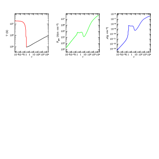
Figure 1: Vertical structure of the hot layer on top of an accretion disc at $r=10\,r_{\rm g}$, for $M=10^{7}\,{\rm M}_{\odot}$, $\dot{m}=0.05$, $\alpha=0.1$, $\xi=0.5$ and $\eta=1$. Plotted are the gas temperature, gas pressure and density. Sharp transition between the upper, hot, ionized layer and cool disc is observed. The thickness of the hot layer (from $T_{\rm s}\approx T_{\rm IC}$ to $7/15\,T_{\rm s}$) is $\tau_{\rm hot}\approx 0.1$. The non-monotonicity of $P_{\rm gas}$ and $\rho$ is due to contribution to energy transfer from vertical convection, and contribution from radiation pressure.

The model parameter crucial for spectral/timing predictions is the thickness of the hot layer, $\tau_{\rm hot}$. The larger the thickness, the smaller the fraction of primary radiation penetrating to the cold layer and giving rise to the usual reprocessed component. The reprocessed component is further Comptonized as the photons escape through the hot layer. The result (at least in the limited energy band corresponding to e.g. Ginga or RXTE data) is a reprocessed component with amplitude reduced compared to the usual geometrical factor $\Omega/4\pi$ (Eq. 8), where $\Omega$ is the solid angle subtended by the reprocessor from the X–ray source (Done & Nayakshin 2001). The amplitude of the iron spectral features is further reduced by the Comptonization.

Two most important parameters determining the thickness of the hot layer are: the strength of irradiation compared to internal disc emission, $F_{\rm X}/F_{\rm D}$, and the ratio of gravity at the base of the layer to X–ray radiation pressure (RC96, NKK). Following NKK we parameterize the latter by

$$A\equiv{\mu_{\rm m}\over m_{\rm e}}{r_{\rm g}\over r}\left({H_{\rm d}\over r}\right)^{2}l_{\rm X}^{-1},$$ (4)

where

$$l_{\rm X}\equiv{F_{\rm X}H_{\rm d}\sigma_{\rm T}\over m_{\rm e}c^{3}},$$ (5)

where $\mu_{\rm m}=\rho/n_{\rm H}\approx 1.9$ for cosmic abundance. Obviously then, the structure of the hot layer has to be solved simultaneously with the structure of the cold disc, since $A$ depends on the disc thickness, $H_{\rm d}$. NKK used vertically averaged solutions of Shakura & Sunyaev (1973; hereafter SS) for the disc in their computations of $\tau_{\rm hot}$. They assumed that total pressure, $P_{\rm gas}+P_{\rm rad}$, should be continuous across the boundary between the two layers, and obtained both $P_{\rm gas}$ and $P_{\rm rad}$ individually continuous across the boundary.

In this paper we explicitly solve equations of vertical structure of the cold disc. We do this for the $\alpha P_{\rm tot}$ SS disc, i.e. a disc with energy generation proportional to total pressure. We define the input parameters of the computations in such a way as to make the connection between accretion discs models and observable quantities obvious. First, we describe calculations at a given radius and then discuss radial dependence of $\tau_{\rm hot}$.

3.1 Vertical structure at a given radius

The structure of the HL at a given radius is computed by combining the method of RC96 and R99 with computations of the vertical structure of X-ray illuminated discs by Różańska et al. (1999). For the HL we follow closely the method of RC96 and R99, with the important simplification of neglecting thermal conduction. The reason is purely practical, as efforts to fully combine proper photo-ionization computations of the hot layer with vertical disc structure have only just begun (Dumont, Abrassart & Collin 2000; Różańska et al., in preparation). This leaves us with an important problem of selecting proper solution in the zone of instability, where the system of equations has more than one solution for temperature. We adopt a simple prescription and select the highest value of $T$ as the solution. Comparing solutions with and without conduction in RC96 and R99 one sees that our procedure may overestimate somewhat the total thickness of the hot and transition layers (i.e. the depth of the point where $T=T_{\rm eff}$). However, the thickness of the hot layer alone is not affected by our neglecting the thermal conduction. The spectrum of illuminating radiation is assumed to be a power law with a cutoff, $F_{E}\propto E^{-\Gamma+1}{\rm e}^{-E/E_{\rm c}}$, parameterized by the photon spectral index $\Gamma$ and cutoff energy, $E_{\rm c}$.

Equations of vertical structure of the cold disc are the same as in Różańska et al. (1999). We assume that a certain fraction of gravitational energy, $\xi$, is dissipated within the disc (but the disc transports all the angular momentum, see e.g. Witt, Czerny & Życki 1997). The remaining fraction, $1-\xi$, is dissipated in an active corona and converted to hard X-ray radiation, of which a fraction $0.5\eta$ illuminates the disk, i.e.

$$F_{\rm X}=0.5\eta(1-\xi)F_{\rm tot},$$ (6)

where

$$F_{\rm tot}=G(r)\equiv{3\over 8\pi}{GM{\dot{M}}\over r^{3}}\left(1-\sqrt{{6r_{\rm g}\over r}}\right),$$ (7)

is the gravitational energy dissipation per unit area of the disc surface. Value of $\eta=1$ would thus correspond to a stationary illumination by an X-ray producing corona above the disk, assuming isotropic emission (see e.g. Haardt & Maraschi 1991). We will assume $\eta\geq 1$, corresponding to a possible enhancement of the X–ray flux. Such an enhancement can be expected if the X–rays are produced by magnetic flares, due to 1) the “charge” time of a flare being longer than the “discharge” time, 2) the collecting area for the flare energy being larger than the illuminated area (e.g. Haardt, Maraschi & Ghisellini 1994).

We solve the structure of the HL assuming a certain initial geometrical thickness of the total system, $H_{\rm tot}$. Four parameters, computed at the bottom of the HL, are then used to modify the equations of the disc structure and their boundary conditions:

• Location of the bottom of the HL (height above the equatorial plane) gives the initial thickness of the cold disc,

• The hard X-ray flux attenuated by the HL contributes to heating of the disc.

• The temperature at the top of the cold disc is computed from the Eddington approximation, $T=T_{\rm eff}[1/2+(3/4)\,\tau]^{1/4}$, taking $\tau$ to be equal to the optical depth of the HL, and $T_{\rm eff}$ from both the internal energy dissipation and the irradiation,

• Gas pressure at the bottom of the HL determines the gas density at the top of the disk.

Iterations of the vertical structure of the disc now follow, to compute the disc thickness for given disc dissipation $\xi F_{\rm tot}$, with the boundary conditions as above. Usually, the converged thickness of the disc is different than the initially assumed one. Therefore the final solution (at a given radius $r$ and for an assumed central mass $M$, mass accretion rate $\dot{m}\equiv{\dot{M}}/\dot{M}_{\rm Edd}$, and viscosity parameter, $\alpha$) is obtained by iterating $H_{\rm tot}$ until a consistent solution is found. As already mentioned above, we define $\tau_{\rm hot}$ as the thickness of the layer where temperature changes from $T_{\rm s}$ down to $(7/15)\,T_{\rm s}$.

As a reference, we compute $\tau_{\rm hot}$ for parameters appropriate for a Seyfert 1 galaxy: $M=10^{7}\,{\rm M}_{\odot}$, $\dot{m}=0.05$, $r=10\,r_{\rm g}$ (close to the peak in energy dissipation), $\alpha=0.1$, $\xi=0.5$ and $\eta=1$ (i.e. no enhancement), $\Gamma=1.9$ and $E_{\rm c}=150$ keV.

Figure 1 shows an example of the vertical structure of the disc with the hot layer. The Thomson thickness of HL is rather small, $\tau_{\rm hot}\approx 0.1$, irrespectively of $\alpha$. The “gravity parameter” is $A\approx 7$ in this case. Our value of $\tau_{\rm hot}$ is thus very similar to what NKK obtain for this value of $A$ (see fig. 4 in NKK), demonstrating that, despite some approximations in our procedure, our results are accurate.

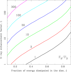
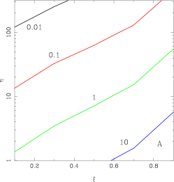
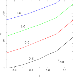
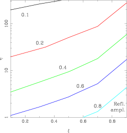
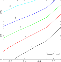
Figure 2: Results of computations of the structure of the hot layer on top of an accretion disc at $r=10\,r_{\rm g}$, for $M=10^{7}\,{\rm M}_{\odot}$, $\dot{m}=0.05$ and viscosity parameter $\alpha=0.1$. The panels show contours of: $F_{\rm X}/F_{\rm D}$ – the ratio of the illuminating X–ray flux to the disc flux due to internal dissipation; $A$ – the gravity parameter (see equation 4); $\tau_{\rm hot}$ – the Thomson thickness of the hot layer; the effective amplitude of the cold, reprocessed component (equation 8); $F_{\rm hard}/F_{\rm soft}$ – the ratio of the observed hard X–ray flux to the soft, thermal flux.

The main parameter, $A$, is a non-unique function of other parameters of the system. For given $\dot{m}$ and $r$, $A$ is determined by a combination of $\xi$ and $\eta$: both parameters influence the disc thickness and the irradiation flux. We have therefore extended our reference computations to obtain $\tau_{\rm hot}$ on a grid of $\xi$ and $\eta$. Results are plotted in Figure 2, where we show a number of quantities characterizing the disc or the spectrum.

The amplitude of the observed “cold” reflection (energy-integrated albedo) is estimated using

$$R={\left[p_{\rm tr}(\tau_{\rm hot})\right]^{2}\over 1+p_{\rm rf}(\tau_{\rm hot})},$$ (8)

where $p_{\rm tr}(\tau_{\rm hot})$ and $p_{\rm rf}(\tau_{\rm hot})$ are hard X–rays transmission and reflection probabilities for the HL thickness $\tau_{\rm hot}$. They are defined as ratios of the transmitted and reflected flux to the incident flux, respectively, for a purely scattering atmosphere. The factor $p_{\rm tr}^{2}$ appears in the numerator of equation (8), because the reflected photons have to go through the HL twice. Additionally, a fraction $p_{\rm rf}$ of the incident photons is elastically back-scattered off the HL, and, by our assumption, simply contributes to the primary continuum photons initially directed towards an observer. In the limiting case of no HL ($\tau_{\rm hot}\rightarrow 0$), $p_{\rm tr}(\tau_{\rm hot})\rightarrow 1$, while $p_{\rm rf}(\tau_{\rm hot})\rightarrow 0$ and $R\rightarrow 1$, i.e. $R$ represents then the solid angle of the reprocessor, $\Omega$, normalized to $2\pi$. We compute $p_{\rm tr}(\tau_{\rm hot})$ and $p_{\rm rf}(\tau_{\rm hot})$ using a Monte Carlo simulations of Compton scattering. This is a rather approximate estimate of the angle averaged amplitude, since it assumes no photo-absorption in the HL, i.e. no contribution to the reprocessed spectrum from highly (but not completely) ionized elements. It thus assumes a rather hard illuminating spectrum ($\Gamma<2$) giving high $T_{\rm IC}$. A more accurate procedure of estimating $R$ was employed by Done & Nayakshin (2001), who fitted spectra computed by NKK by a “cold” reflection model in the context of Ginga data. For softer illuminating spectra, $\Gamma\ga 2$, the reprocessed component contains strong spectral features due to H- and He-like Fe ions and it cannot be approximated by “cold” reprocessing (NKK; Nayakshin 2000b).

The ratio $F_{\rm hard}/F_{\rm soft}$ is the observed ratio of fluxes, i.e. the hard X–ray flux

$$F_{\rm hard}=F_{\rm X}(1+p_{\rm rf})$$ (9)

contains a contribution from photons backscattered in the HL towards an observer. The soft flux, $F_{\rm soft}$, contains a contribution from the disc internal emission, $F_{\rm D}=\xi F_{\rm tot}$, and hard photons thermalized in the cold disc,

$$F_{\rm soft}=F_{\rm D}+(1-a)p_{\rm tr}F_{\rm X},$$ (10)

with $a\approx 0.2$ being the energy-integrated X–ray albedo of cold matter. We note that the above relations of $F_{\rm hard}$ and $F_{\rm soft}$ with $F_{\rm X}$ assume implicitly that there are no significant changes of the source geometry (e.g. the height of the flare above the disc), so that the variability of $F_{\rm X}$ is solely due to the variable output of the magnetic activity.

The structure of the disc has to be rather different from the standard SS solution, if the hot layer is to be Thomson thick(ish), $\tau_{\rm hot}\ga 1$. For half of the total energy dissipated in the active regions, $\xi=0.5$, the illumination flux has to be further enhanced by a factor of $\eta\approx 40$ relative to the stationary situation in order to obtain $\tau_{\rm hot}=1$. This corresponds to the ratio of illumination flux to disc internal flux, $F_{\rm X}/F_{\rm D}=0.5\eta(1-\xi)/\xi\approx 20$. For larger fraction of energy dissipated in the magnetic corona, i.e. smaller $\xi$, the required ratio $F_{\rm X}/F_{\rm D}$ is even larger (e.g. $F_{\rm X}/F_{\rm D}\approx 60$ for $\xi=0.1$). This appears to be due to the disc thickness, $H_{\rm d}$, increasing with $\xi$ more slowly than linearly, and thus for $A\propto(F_{\rm D}/F_{\rm X})(H_{\rm d}/\xi)$ to remain constant, $F_{\rm X}/F_{\rm D}$ has to increase when $\xi$ decreases.

On the other hand, the presence of the HL will be apparent in observations even if its thickness is rather smaller than $\tau_{\rm hot}=1$. According to our approximate formula (equation 8) reflection amplitude gets reduced to 0.8 for $\tau_{\rm hot}\approx 0.25$. Quality of current data is usually sufficient to distinguish $R=0.8$ from $R=1$ in typical X–ray spectra of AGN (e.g. Done et al. 2000).

3.2 Radial structure

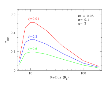
Figure 3: Thomson thickness of the hot layer as a function of radius for $\eta=3$ and three values of $\xi$, as labelled. Other parameters: $M=10^{7}\,{\rm M}_{\odot}$, $\dot{m}=0.05$ and $\alpha=0.1$.

The Thomson thickness of the HL changes with radius, even for a constant $F_{\rm X}/F_{\rm D}$, since $A$ is not constant with $r$. We computed radial dependencies of $\tau_{\rm hot}$ for $\eta=3$ and three values of $\xi=0.01,0.3$ and $0.6$. Values of other parameters were as before: $M=10^{7}\,{\rm M}_{\odot}$, $\dot{m}=0.05$, $\alpha=0.1$. Results are plotted in Fig. 3.

The thickness is largest at $r\approx 10\,r_{\rm g}$. It then drops slowly, roughly in accord with the formula of Nayakshin (2000a). A consequence of that particular $\tau_{\rm hot}(r)$ distribution is a relative suppression of highly relativistically smeared component of the reprocessed spectrum. On the other hand, the reprocessed photons that do manage to diffuse from below the hot layer close to the central BH, suffer Comptonization smearing, which in practice may be difficult to distinguish from relativistic smearing (see Sec. 5.2).

Obviously, in the magnetic flare scenario there is no reason for changes of $\xi$ and $\eta$ to be perfectly correlated on all radii. One can thus imagine rather different values at different radii, leading to $\tau_{\rm hot}(r)$ rather different than those plotted in Fig. 3. On timescales long compared to $t_{\rm dyn}$ one could perhaps obtain time average $\xi(r)$ and $\eta(r)$ employing a particular variability model, e.g. that of Poutanen & Fabian (1999).

3.3 Dependence of ${\boldmath\tau_{\bf hot}}$ on X–ray flux

The qualitative relation between the thickness of the HL and the illuminating X–ray flux is obvious: the stronger the X–ray flux the thicker the HL. In this Section we present the quantitative relation from our model.

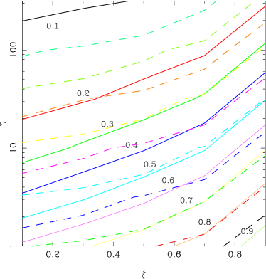
Figure 4: Upper panel: contours of observed amplitude of the reprocessed component (solid curves, labelled), and contours of observed hard X–ray flux (dashed curves). Each contour of $F_{\rm hard}$ means an increase of $F_{\rm hard}$ by a factor of 2. Lower panel: projected dependence of $R$ vs. $F_{\rm hard}$. Clearly, the dependence is much weaker than linear, i.e. it is not possible for the absolute normalization of the reprocessed component, $N=R\times F_{\rm hard}$ to remain constant. See Figure 2 for parameters of computations.

In Figure 4 we again plot contours of amplitude of reflection $R$ in the $\xi$–$\eta$ plane, together with contours of the observed X–ray flux, $F_{\rm hard}$, as well as the projected dependence $R$–$F_{\rm hard}$. For $R$ close to 1, doubling $F_{\rm X}$ results in only modest decrease of $R$, by 10–20 per cent. For smaller $R$ the process is more effective. But still, to go from e.g. $R=0.8$ to $R=0.4$ requires an increase of $F_{\rm hard}$ by a factor of $\ga 8$ (when the movement is along the $\xi$ axis, for $\eta\approx 4$). Going from $R=0.6$ to $R=0.3$ requires that $F_{\rm hard}$ increases at least 4 times, again approximately along the $\xi$ axis. In no case does it seems possible to obtain an inverse proportionality of $F_{\rm hard}$ and $R$, so that $R\times F_{\rm hard}\approx{\rm const}$. Thus, these results seem to rule out the possibility that the absolute flux of the Fe K_α line may remain constant despite continuum variability, although certain reduction of the line variability amplitude (compared to that of the continuum) can be expected (see next Section).

We note that a change of $F_{\rm X}$ is more effective in changing $\tau_{\rm hot}$, if $F_{\rm X}$ increases or decreases due to changing fraction of energy dissipated in the disc, $\xi$, rather than $\eta$. The reason is that e.g. removing the energy dissipation from the disc to the active corona (i.e. decreasing $\xi$) not only increases the X–ray illuminating flux, but it also decreases the disc thickness, thus decreasing the gravity.

4 Reduction of variability amplitude of the Fe K_α line

4.1 Method

Based on results of previous Section we expect the variability of the Fe K_α line flux to be reduced compared to the amplitude of variability of the driving continuum, even though it does not seem possible to obtain absolutely constant flux of the line. Here we estimate the reduction of the r.m.s. variability of the Fe K_α line, compared with an assumed r.m.s. variability of its driving continuum. To this end we will use results of our calculations of $\tau_{\rm hot}(\xi,\eta)$ at $r=10\,r_{\rm g}$. In this way we will obtain the upper limit to the considered effect, since $\tau_{\rm hot}(r)$ reaches maximum at $r\approx 10\,r_{\rm g}$, for a given pair $(\xi,\eta)$ (see Fig. 3).

First, we construct a simulated light curve of hard X–ray continuum by summing Fourier components with random phases (e.g. Tsonis 1992),

$$C(t_{i})=\sum_{j=1}^{N}\sqrt{P(f_{j})}\cos\left[2\pi f_{j}t_{i}+\phi(f_{j})\right],$$ (11)

for an adopted form of power spectral density (PSD), $P(f)$. For the PSD we adopt

$$P(f)\propto{1\over\left[1+(f/f_{\rm c})\right]^{p}}.$$ (12)

This provides a good description of hard X–ray PSD of e.g. MCG–6-30-15, with the cutoff frequency $f_{\rm c}=10^{-5}$ Hz, the slope $p=1.4$ and the normalization corresponding to r.m.s. variability of 20 per cent (Green, McHardy & Lehto 1993; Czerny & Lehto 1997; Yaqoob et al. 1997; Nowak & Chiang 2000; Reynolds 2000). We take these parameters to be representative for Seyfert 1 galaxies. The light curve is scaled to have a given mean value ${\overline{C}}$. Next, the light curve in energy band containing the K_α line photons is constructed according to

$$L(t_{i})=(1-A_{\rm l})C(t_{i})+A_{\rm l}C(t_{i})R[C(t_{i})],$$ (13)

where $A_{\rm l}$ is the fraction of line photons contributing to total counts in the considered energy band, while $R[C(t)]$ is the relative amplitude of the reprocessed component as a function of the illuminating hard X–ray flux. Writing equation (13) we have assumed no time lag in the response of the Fe K_α line emission after the continuum variations, consistent with observations (e.g. Reynolds 2000). The amplitude $R[C(t)]$ is computed as follows: we choose a value for the effective amplitude of the reprocessed component at the mean flux level, $R({\overline{C}})$. We then assume that $R({\overline{C}})$ corresponds to a pair $(\xi_{0},\eta_{0})$, which is located on a trajectory in the $\xi$–$\eta$ plane that the system travels while changing its luminosity. The trajectory describes how changes of $\xi$ and $\eta$ contribute to the variability. Since our understanding of variability mechanisms is rather limited, we will simply test a number of arbitrary trajectories, to get an idea of available range of results. As discussed in previous Section, variations along the $\xi$-axis give largest possible change of $R$ for a given change of $F_{\rm X}$, therefore our chosen trajectories have a significant component along the $\xi$ axis.

Next, we construct the light curve of the observed hard X–ray continuum, which has a contribution from photons backscattered in the hot layer, i.e. $F(t)=C(t)\{1+p_{\rm rf}\{\tau_{\rm hot}[C(t)]\}\}$. Finally, the r.m.s. variability is computed for $F(t)$ and $L(t)$ according to

$$\sigma_{\rm var}(C)={1\over{\overline{C}}}{\sqrt{{1\over N}\sum_{i=1}^{N}\,\left[C(t_{i})-{\overline{C}}\right]^{2}}}.$$ (14)

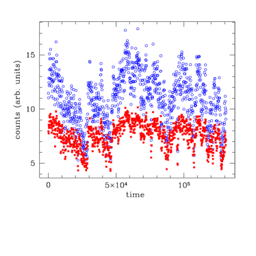
Figure 5: Examples of light curves of the observed hard X–ray continuum (open circles) and the Fe K_α line (solid squares), simulated from the PSD defined in Sec 4.1. The assumed parameters gave the effective amplitude of the reprocessed component $R({\overline{C}})\approx 0.75$. In effect the line flux is suppressed at almost all times and reduction of the line r.m.s. variability is significant, at 6 per cent (see Fig. 6).

4.2 Results

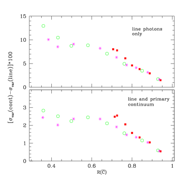
Figure 6: Amplitude of variability of the Fe K_α line flux is reduced compared the that of the driving continuum, due to appearance of a hot, ionized layer with thickness increasing with increasing illuminating flux. This is plotted here as a function of the assumed effective amplitude of reflection at the mean flux level. Upper panel shows reduction of the r.m.s. variability assuming that there are no primary continuum photons in the line energy band. Lower panel shows analogous reduction assuming that the line photons contribute 15 per cent to the considered energy band. Different symbols denote different trajectories in the $\xi$–$\eta$ plane traveled by the varying system. The r.m.s. variability of the driving continuum was 20 per cent. See text (Sec 4.2) for further explanations.

First we set $A_{\rm l}=1$ i.e. we consider the light curve of the Fe K_α line alone, without any continuum photons. An example of the simulated light curves is plotted in Fig. 5. They were obtained assuming that the mean flux of the intrinsic continuum, $\overline{C}$, corresponds to $\xi_{0}=0.5$ and $\eta_{0}=1$ (which yields $R({\overline{C}})\approx 0.75$, see Fig. 4), and that the variability is only due to changing $\xi$. The line flux is reduced at all times, since $R({\overline{C}})$ is significantly lower than 1, and its r.m.s. variability is reduced by $\approx 5$ per cent compared with the r.m.s. variability of its driving continuum, $C(t)$. The observed hard X–ray continuum, $F(t)$, contains a contribution from photons backscattered in the hot layer, which increase its r.m.s. variability by $\approx 1$ per cent. Thus, the difference of r.m.s. variabilities between the line and the hard continuum, $\sigma_{\rm var}(F)-\sigma_{\rm var}(L)$ is in this example $\approx 6$ per cent.

In real spectra the contribution of line photons to the 5–7 keV band is only $A_{\rm l}\approx 0.15$, for $R=1$. The reduction of r.m.s. variability, $\Delta\sigma_{\rm var}\equiv\sigma_{\rm var}(F)-\sigma_{\rm var}(L)$, is therefore much weaker than in previous case, and in the above example, only $\approx 2$ per cent.

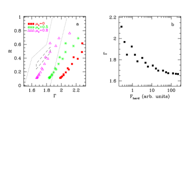
Figure 7: Panel a): the amplitude of reflection – spectral index correlation predicted by the model for a number of $\mu_{\rm s}$ values (equation 16). Only models with $\xi\leq 0.5$ were used (most of the energy dissipated in the active corona). The contours represent the observed correlations (Zdziarski et al. 1999; Gilfanov et al.  2000). Panel b) shows hard X–ray flux – spectral index anti-correlation. Each “triplet” of points corresponds to a given value of $\eta$ and $\xi=0.1,\ 0.3,\ 0.5$. The anti-correlation, which has an obvious physical interpretation in this model, seems to be opposite to what is observed in the data (e.g. Done et al. 2000).

The difference $\Delta\sigma_{\rm var}$ is plotted in Fig. 6 as a function of $R({\overline{C}})$, for both $A_{\rm l}=1$ and $A_{\rm l}=0.15$. The general trend is that the larger the $R({\overline{C}})$ is, the smaller the $\sigma_{\rm var}(F)-\sigma_{\rm var}(L)$ is. Consider for example $R({\overline{C}})\approx 1$, i.e. at the mean flux level the irradiation flux is relatively weak and in consequence the hot layer is rather thin, $\tau_{\rm hot}\leq 0.1$. Then $R$ is reduced only when the instantaneous flux exceeds the mean flux, but $R$ saturates at 1 whenever $C(t)<{\overline{C}}$. This then gives smaller reduction of r.m.s. variability compared to a case $R({\overline{C}})\sim 0.5$ when the anti-correlation between $R$ and $C(t)$ can hold through the entire range of $C(t)$. Details of the relation $R({\overline{C}})$–$\Delta\sigma_{\rm var}$ depend on the mapping $C(t)\rightarrow(\xi,\eta)$, i.e. which parameter, $\xi$, $\eta$ or both of them, cause flux variations. Solid squares in Fig. 6 show the case of variations $C(t)$ caused by changes of $\xi$ only (for $\eta=1$). Reduction of the line variability is strongest in this case, since a given variation of $C(t)=F_{\rm X}$ causes largest possible change of $R$, as already discussed in Sec. 3.3 and shown in Fig. 4. On the other hand, the available range of $R({\overline{C}})$ is rather limited.

These results are quantitatively dependent on the assumed constancy of X–ray source geometry (see comments following Eq. (10)). The reduction of variability, $\Delta\sigma_{\rm var}$, could be larger, if the geometry were correlated with the X–ray luminosity, changing in such a way as to make the illuminating flux, $F_{\rm X}$, to increase more strongly than the observed flux, $F_{\rm hard}$. However, as we are going to argue in the next Section, the combined timing and spectral observational result put quite tight constraints on any geometry–luminosity dependences.

Finally, we note that both $R({\overline{C}})$ and $\sigma_{\rm var}(F)-\sigma_{\rm var}(L)$ are observable quantities and their relation plotted in Fig. 6 can be used to test the model.

5 Spectral Data

5.1 The ${\boldmath R}$–${\boldmath\Gamma}$–flux correlations

The spectral index of the hard X–ray power law, $\Gamma$, and the observed amplitude of the reprocessed component, $R$, appear to be correlated in the data of both AGN and Galactic Black Holes (GBH) (Zdziarski, Lubiński & Smith 1999; Gilfanov, Churazov & Revnivtsev 2000): the harder the spectrum (smaller $\Gamma$), the smaller the amplitude. Two models were considered to explain the correlation: truncated cold disc with hot central flow (e.g. Esin, McClintock & Narayan 1997) and relativistic outflow of emitting plasma (Beloborodov 1999ab). The model of an accretion disc with a hot layer is also able to qualitatively explain the correlation, with $\tau_{\rm hot}$ being the control parameter: the larger $\tau_{\rm hot}$ is, the smaller the effective $R$ and the harder the spectrum, due to reduced soft flux from thermalization (assuming that most of the energy dissipation occurs in the active corona). We present here the $R$–$\Gamma$ correlation predicted by the model. The estimate of $R$ is obtained as in Sec. 3.1 (equation 8), while for $\Gamma$ we use the formula from Beloborodov (1999ab),

$$\Gamma\approx 2.33(l_{\rm h}/l_{\rm s}-1)^{-1/10},$$ (15)

where $l_{\rm h}$ and $l_{\rm s}$ are the power in hard and soft radiation crossing the active region, respectively. We estimate

$$l_{\rm s}=\int_{-1}^{-\mu_{\rm s}}[F_{\rm dissip}(\mu)+F_{\rm reproc}(\mu)]\,d\mu,$$ (16)

where $F_{\rm dissip}\equiv F_{\rm D}=\xi F_{\rm tot}$ and

$$F_{\rm reproc}=(1-a)F_{\rm X}={1\over 2}\eta(1-\xi)(1-a)F_{\rm tot}\,p_{\rm tr}\left(\tau_{\rm hot}(\xi,\eta)\right).$$ (17)

The second term describes the contribution to the soft flux from the thermalized fraction of the illuminating X–rays. We have also introduced the geometrical factor $\mu_{\rm s}$ (see Beloborodov 1999ab), describing the fraction of soft flux actually intercepted by a magnetic flare (in computations we assume isotropic emission). The hard power is simply estimated as $l_{\rm h}=2F_{\rm X}=\eta(1-\xi)F_{\rm tot}$.

Figure 7 presents results of the computations for a number of $\mu_{\rm s}$ values. The shape of the model correlation is somewhat different from the correlation observed in the data. The model requires $\mu_{\rm s}>0.6$ in order to obtain quantitative agreement with the data, i.e. $1-\mu_{\rm s}<0.4$ of the soft flux crossing an active region. It has to be remembered however that the observed correlation, particularly among different objects, is more likely to be due to changes of geometry driven by e.g. $\dot{m}$ rather than varying output of magnetic activity, and thus parameterizing the correlation by our parameters $\xi$ and $\eta$ may not be sufficient.

Another correlation applicable to AGN observations may be the $F_{\rm hard}$–$\Gamma$ (anti)correlation plotted in Figure 7b. It follows from combining results shown in Fig. 4 with those in Fig. 7: an increase of illuminating flux, $F_{\rm X}$, gives a decrease of $R$ and a decrease of $\Gamma$. If the observed X–ray flux, $F_{\rm hard}$, follows the illuminating flux, $F_{\rm X}$, (i.e. if the Eq. (9) holds), the predicted $F_{\rm hard}$–$\Gamma$ anticorrelation is obtained. However, an opposite effect seems to be observed in the data from RXTE observing campaigns of some AGN, where the spectrum generally softens ($\Gamma$ increases) when the observed X–ray flux goes up (NGC 5548, Chiang et al. 2000; IC 4329a, Done et al. 2000). At least in IC 4329a the spectral analysis of Done et al. (2000) reveals that this is not an artifact of limited band pass of RXTE instruments. If this observational result is generic, it would mean changes of the flares’ geometry correlated with their luminosity, so that the relation between $F_{\rm hard}$ and $F_{\rm X}$ can be reversed. From the discussion of variability (Sec 4.2), we need a correlated increase of $\tau_{\rm hot}$ with the flare luminosity. If this is to be accompanied by a softening of the spectrum, the flare’s geometry has to change in such a way, that the intercepted soft luminosity is larger than the increased hard luminosity ($l_{\rm h}/l_{\rm s}$ has to decrease; Eq. (15)), despite the decreased soft flux from thermalized hard X–rays.

5.2 Model dependence of relativistic smearing and amplitude of reflection

The hot layer is thickest at close distances from the central black hole, according to results of computations of $\tau_{\rm hot}(r)$ presented in Sec. 3.2. The K_α line generation is then suppressed at small $r$, which means that the inner disc radius determined from the line profile may be larger than $r_{\rm ms}=6\,r_{\rm g}$. We quantified this effect in our model, since indeed the line observed in a number of sources is narrower than in the extreme case of MCG–6-30-15 (IC 4329a, Done et al. 2000; Cyg X-1, Done & Życki 1999; GS 2023+338, GS 1124-68, Życki, Done & Smith 1997, 1998).

We computed the relativistic smearing in the reprocessed spectra for the radial dependencies $\tau_{\rm hot}(r)$ plotted in Fig. 3. We assumed that the irradiation emissivity follows radial distribution of gravitational energy dissipation, G(r) (equation 7). Ratios of the reprocessed spectra to the reference case of no hot skin (so full relativistic smearing), are plotted in Fig. 8. The magnitude of the effect obviously depends on the thickness of the HL. Even for the thickest HL considered ($\xi=0.01$, maximum $\tau_{\rm hot}(r)\approx 0.5$), the “wiggles” in the ratio plots are only a few percent, for pure reprocessed component, i.e. no contribution from primary photons. It would then be rather difficult to detect such an effect in the data, the more so that the additional broadening due to Comptonization in the HL (not included here), is strongest for the thickest HL. Qualitatively then, reduction of effective amplitude of the reprocessed component is much more prominent, than any changes to the profile of the K_α line (as is also clear from Fig. 8).

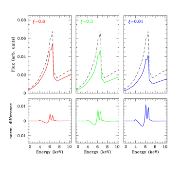
Figure 8: Reprocessed spectra computed for the radial $\tau_{\rm hot}(r)$ dependencies plotted in Fig. 3 (solid lines), compared to the reference case of no hot skin (full relativistic smearing; dashed line). Since $\tau_{\rm hot}(r)$ reaches maximum at $r\approx 10\,r_{\rm g}$, the most strongly relativistically smeared component is suppressed in the spectra. Upper panels show that the main effect is a decrease of the overall amplitude, described by Eq. (8). Lower panel show the difference, $ionized\ skin\ spectrum-reference\ spectrum$, (after correcting for the decrease of amplitude), normalized to the primary power law spectrum. The additional Comptonization broadening of the spectral features is not included.

One can estimate the maximum magnitude of the suppression of the broadest line component, noticing that it will occur for $\tau_{\rm hot}(r)$ being a step function: $\tau_{\rm hot}$ very large for radii $r<r_{\rm cut}$, and $\tau_{\rm hot}=0$ otherwise. In other words, no observable reprocessed component is produced for $r<r_{\rm cut}$ (Ross, Fabian & Young 1999). This obviously means a reduction of the effective amplitude of the reprocessed component, which one can relate to $r_{\rm cut}$

To do so, we write $R=F_{\rm refl}/(a_{0}F_{\rm direct})$, i.e. $R$ is the reflection albedo (ratio of flux of reflected radiation to the flux directed towards an observer), normalized to the albedo $a_{0}$ of cold reflection, expected from an isotropic source above a flat disc. Both fluxes can be written as radial integrals, e.g.

$$F_{\rm refl}=2\pi\int_{r_{\rm min}}^{r_{\rm max}}F_{\rm refl}(r)r\,dr.$$ (18)

Averaged over many dynamical time scales, the radial distribution of energy generation in the active corona can be expected to follow the gravitational energy dissipation prescription. If isotropy of emission is assumed, then

$$F_{\rm refl}(r)=F_{\rm direct}(r)=G(r).$$ (19)

If a purely scattering layer of a thickness giving a transmission probability $p_{\rm tr}$ (reflection probability $1-p_{\rm tr}$) covers the reflecting disc up to a radius $r_{\rm cut}$, then

$$F_{\rm refl}(r)/a_{0}= 2\pi\int_{r_{\rm min}}^{r_{\rm cut}}p_{\rm tr}^{2}G(r)r\,dr+$$ (20)

$$2\pi\int_{r_{\rm cut}}^{r_{\rm max}}G(r)r\,dr$$

and

$$F_{\rm direct}(r)= 2\pi\int_{r_{\rm min}}^{r_{\rm cut}}(2-p_{\rm tr})G(r)r\,dr+$$ (21)

$$2\pi\int_{r_{\rm cut}}^{r_{\rm max}}G(r)r\,dr.$$

The resulting function $R(r_{\rm cut})$ is plotted in Figure 9 for $p_{\rm tr}=0$, which maximizes $r_{\rm cut}$ for any $R$. For $p_{\rm tr}(r)=1$ (no hot layer) we obviously obtain $R(r_{\rm cut})=1$, but for any $p_{\rm tr}(r)<1$ the amplitude $R$ decreases dramatically with increasing $r_{\rm cut}$, i.e. when the ionized zone becomes more extended. The reason for the dramatic decrease is that the emission is strongly concentrated towards the center. Interestingly, many Galactic black hole binaries show $R\approx 0.3$ and $R_{\rm in}\approx 20\,r_{\rm g}$, in accord with the relation shown in Figure 9, but we note that, with the assumption of perfect reflectivity, the geometry here is equivalent to the disc being truncated at $r_{\rm cut}$, and replaced by central X–ray source. We also emphasize that the assumption $p_{\rm tr}(r<r_{\rm cut})=0$, is not justified by our present understanding of the model.

Figure 9: Relation between effective amplitude of the reprocessed component and the amount of relativistic smearing, for an ad hoc model, where the disc is assumed to be covered by a perfectly reflecting HL (i.e. $\tau_{\rm hot}\gg 1$) from $r_{\rm ms}$ up to a radius $r_{\rm cut}$. This reduces the effective amplitude of reflection and removes the broadest component from the spectral features, with $r_{\rm cut}$ being the inner disc radius as inferred from fitting the profile of the K_α line.

5.3 The X–ray “Baldwin effect”

The observed equivalent width (EW) of the Fe K_α line appears to be anticorrelated with average 2–10 keV luminosities of the sources (Iwasawa & Taniguchi 1993; Nandra et al. 1997), in a similar manner as EW of CIV $\lambda$1550 line is anticorrelated with the UV continuum luminosity (Baldwin 1977). This could be explained by the presence of the hot layer, since indeed $\tau_{\rm hot}$ is larger for larger $F_{\rm X}$, although in this case we expect the flux to be driven by accretion rate, rather than $\xi$ and/or $\eta$. Since the average X–ray luminosity can be expected to be proportional to the accretion rate ${\dot{M}}={\dot{m}}\dot{M}_{\rm Edd}\propto{\dot{m}}M$, we have computed the EW varying either $M$ or $\dot{m}$ and keeping the other parameter constant. We again assumed that situation at $r=10\,r_{\rm g}$ is characteristic to the whole disc, and we adopted $\xi=0.5$ and $\eta=1$. Results presented in Fig. 10 show that indeed the EW of the K_α line ($\propto R$) decreases with $\dot{m}$. The reason for the underlying increase of $\tau_{\rm hot}$ with $\dot{m}$ is that the increase of $H_{\rm d}$ with $\dot{m}$ is slower than linear. The gravity parameter $A\propto H_{\rm d}/{\dot{m}}$ then decreases with $\dot{m}$. We note that the vertically averaged SS solution predicts $H_{\rm d}\propto{\dot{m}}$ and, in consequence, constant $\tau_{\rm hot}$ in the regime of $P_{\rm rad}\gg P_{\rm gas}$ and $\kappa\approx\kappa_{\rm es}$. In our vertically explicit solution $P_{\rm gas}$ is not neglected. Contribution from convective energy transfer contributes to departures from the SS solution as well.

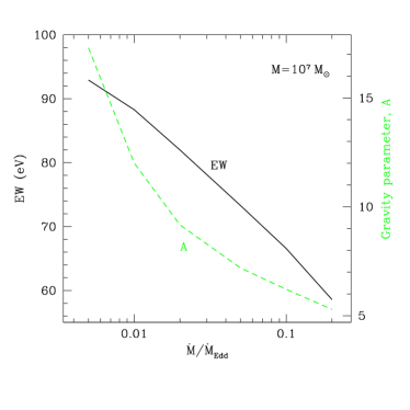
Figure 10: Equivalent width of the Fe K_α line (solid curve, left scale) as a function of the average X–ray source luminosity, $L_{\rm X}$, assuming that $L_{\rm X}\propto\dot{m}$, i.e. $M={\rm const}$. EW decreases with $\dot{m}$ which could explain the observed X–ray “Baldwin effect”. The dotted curve shows the corresponding gravity parameter $A$, which decreases due to slower than linear increase of the disc thickness with $\dot{m}$. Parameters: $M=10^{7}\,{\rm M}_{\odot}$, $\alpha=0.1$, $\xi=0.5$, $\eta=1$.

6 Discussion

Presence of a hot, ionized layer on top of an X–ray illuminated accretion disc has inevitable observational consequences. Most importantly, it reduces the amplitude of the effective, observed “cold” reprocessed component. Since the thickness of the hot layer (hence the reduced amplitude) is correlated with the X–ray flux, a number of observable correlations follow from this model.

Generally, the predicted Fe K_α fluorescent line originating from the disc is weaker (relative to the continuum) when the source is brighter (provided that the illuminating spectrum has $\Gamma<2$ so that there is no He-like Fe in the hot layer; NKK). This effect can be used to explain two observed phenomena. Firstly, the reduction of the amplitude of variability of the line with respect to the driving continuum ($E>7$ keV) in AGN monitoring campaigns (Reynolds 2000; Done et al. 2000; Chiang et al. 2000). Quantitatively, our computations indicate that it is not possible to obtain constant absolute line flux constant. That is, the relative amplitude of the reprocessed component decreases more slowly than $F_{\rm X}^{-1}$. Nevertheless, reduction of the variablity amplitude by a few per cent is possible. However, the variability reduction is inversly related with the mean amplitude of the reprocessed component (i.e. observed at the mean flux level). Thus, in sources like MCG–6-30-15, where $R\approx 1$, this effect should actually be negligible. Moreover, the X–ray continuum in MCG–6-30-15 is rather soft ($\Gamma\ga 2$), which implies a contribution from a highly ionized reprocessed component (NKK), that does not seem to have been observed in this source. Perhaps the hot skin developes on accretion discs in the other Seyfert 1 galaxies, where both $R<1$ and $\sim$constant Fe K_α line flux was observed (IC 4329a, Done et al. 2000; NGC 5548, Chiang et al. 2000). Quality of current RXTE data should be good enough to quantitatively test the model relation presented in Fig. 6.

Second, the decrease of the EW of the Fe K_α line in brighter sources (X–ray “Baldwin effect”) can be explained, if the inverse relation between efficiency of the line production and X–ray flux is applied to a sample of objects. This is not quite a trivial statement, since different average X–ray luminosities of sources are rather due to different mass accretion rates, than a variable output of some magnetic activity.

The model is also able to explain the correlation between the amplitude of the reprocessed component and X–ray spectral index, again observed both in a sample of objects (Zdziarski et al. 1999), and in the time history of a single object (GX 339-4, Gilfanov et al. 2000; GS 1124-68, Życki et al. 1998). Our computations of the correlation give perhaps somewhat different shape to what is observed, although the observed correlation is also subject to instrument–related uncertainties.

Another relation often looked for in data and used to constrain theoretical models is a relation between spectral index and hard X–ray flux. This is usually more difficult to obtain from data because of uncertain corrections from limited detector band pass to the entire X–ray band. Perhaps the most robust result was obtained by Done et al. (2000) for IC 4329a, where broad band spectral analysis revealed that the spectrum became harder when the X–rays ($E>1$ keV) decreased. Similar relation was reported for NGC 5548 (Magdziarz et al. 1998; Chiang et al. 2000) although this involved flux in 2–10 keV band. On the other hand the soft X–ray transient GS 1124-68 (Nova Muscae 1991) showed a clear hardening of its spectrum during its decline phase (Życki et al. 1998; Życki 2001), which was however correlated with an increase of the $E>1\,{\rm keV}$ flux by $\approx 50$ per cent (so called ’re-flare’). The model discussed in this work predicts anti-correlation of $\Gamma$ and $F_{\rm hard}$, i.e. hardening of the spectrum when a source brightens, unless there are correlated changes of the X–ray source geometry and its luminosity.

The structure of the hot layer and resulting correlations between observables may also depend upon the model adopted for the underlying accretion disc. In this paper we adopted the $\alpha P_{\rm tot}$ SS prescription for viscosity. However such discs are subject to a number of instabilities in the parameter range appropriate to AGN. Classical theory predics thermal and viscous instability whenever contribution of gas pressure to $P_{\rm tot}$ drops below 0.4 (Kato, Fukue & Mineshige 1998), which in practice means the region within a few hundreds $r_{\rm g}$, for $\dot{m}$ a few per cent. Therefore, models with a different viscosity prescription were sometimes considered, e.g. $\alpha P_{\rm gas}$, which are free from those instabilities. Solving the vertical structure of $\alpha P_{\rm gas}$ discs for a number of ($\xi,\ \eta$) values we find that the disc height is very similar (less than 1 per cent difference) to that of the corresponding $\alpha P_{\rm tot}$ disc. The resulting relations between observable quantities are then practically identical to those for $\alpha P_{\rm tot}$ discs. Our current understanding of mechanisms providing viscosity strongly points out towards the magneto-rotational instability as the source of turbulence responsible for the viscosity (see Balbus & Hawley 1998 for review). Global magnetohydrodynamical simulations reveal the disc structure very different from the smooth, classical, hydrodynamical models (Hawley 2000). The spatial and temporal structure is highly turbulent and inhomogeneous, displaying fractal-like scalings (Kawaguchi et al. 2000). The relevance of the presented model to such inhomogeneous, clumpy discs needs further studies.

The presented model is currently one of at least three general scenarios within which it is possible to explain bulk of observed data from low/hard states of AGN and GBH: the other two are the cold disc with inner hot flow model (Esin et al. 1997 and references therein; Różańska & Czerny 2000b) and relativistically outflowing plasma model (Beloborodov 1999ab). None of them fully addresses all complexities of observed spectral and timing data, but all three account for the main facts: the range of observed spectral indices, the $R$–$\Gamma$ correlation, relativistic smearing of Fe reprocessed features (see Poutanen 1998 for review and e.g. Di Salvo et al. 2001 for application to Cyg X-1). It also seems possible to incorporate into all of them the basic X–ray timing observables: the shape of PSD, time lags, auto- and cross-correlation functions (Poutanen & Fabian 1999; Böttcher & Liang 1999; see review in Poutanen 2000). Clearly, further progress can only be made if the models are developed in more details incorporating more relevant physical processes. Confronting detailed, quantitative predictions with good quality spectral and timing data should hopefully enable distinguishing which, if any, of our current ideas are closest to reality.

7 Conclusions

• The model does predict certain reduction of the variability of the Fe K_α line, compared to the variability of its driving continuum, although it does not seem possible to obtain absolutely constant line flux.

• The anti-correlation of the equivalent width of the K_α line and average source luminosity (the X–ray “Baldwin effect”) is reproduced in the model.

• Reduction of the amplitude of the observed, “cold” reprocessed component is more evident than any reduction of the spectral broadening (due to relativistic effects and Comptonization) of the K_α line.

• The model is able to quantitatively explain the observed $R$-$\Gamma$ correlation.

• The geometry of the X–ray sources is quite tightly constrained, if the model is to explain both timing and spectral observational data.

References

- [] Balbus S. A., Hawley J. F., 1998, Rev. Mod. Phys., 70, 1
- [] Baldwin J. A., 1977, ApJ, 214, 679
- [] Beloborodov A. M., 1999a, ApJ, 510, L123
- [] Beloborodov A. M. 1999b, in Poutanen J., Svensson R. eds, ASP Conf. Ser. 161, High Energy Processes in Accreting Black Holes, 295, (astro-ph/9901108)
- [] Blandford R. D., McKee C. F. 1982, ApJ, 255, 419
- [] Böttcher M., Liang E. P. , 1999, ApJ, 511, L37
- [1] Chiang J., Reynolds C. S., Blaes O. M., Nowak M. A., Murray N., Madejski G. M., Marshall H. L., Magdziarz P., 2000, ApJ, 528, 292
- [] Czerny B., Lehto H. J., 1997, MNRAS, 285, 365
- [2] Di Salvo T., Done C., Życki P. T., Burderi L., Robba N. R., 2001, ApJ, 547, 1024
- [] Done C., Nayakshin S., 2001, ApJ, 546, 419
- [] Done C., Życki P. T., 1999, MNRAS, 305, 457
- [] Done C., Madejski G. M., Życki P. T., 2000, ApJ, 536, 213
- [] Dumont A.-M., Abrassart A., Collin S., 2000, A&A, 357, 823
- [] Esin A. A., McClintock J. E., Narayan R. 1997, ApJ, 489, 865
- [] Fabian A. C., Nandra K., Reynolds C. S., Brandt W. N., Otani, C., Tanaka, Y., Inoue, H., Iwasawa, K., 1995, MNRAS, 277, L11
- [] Field G. B., 1965, ApJ, 142, 531
- [] Gilfanov M., Churazov E., Revnivtsev M., in Proc. of the 5th CAS/MPG Workshop on High Energy Astrophysics, 2000, in press, (astro-ph/0002415)
- [] Green A. R., McHardy I. M., Lehto H. J., 1993, MNRAS, 265, 664
- [] Haardt F., Maraschi L., 1991, ApJ, 380, L51
- [] Haardt F., Maraschi L., Ghisellini G., 1994, ApJ, 432, L95
- [] Hawley J. F., 2000, ApJ, 528, 462
- [] Iwasawa K., Taniguchi Y., 1993, ApJ, 413, L15
- [] Iwasawa K. et al. 1996, MNRAS, 282, 1038
- [] Karas V., Czerny B., Abrassart A., Abramowicz M. A., 2000, MNRAS, 318, 547
- [] Kato S., Fukue J., Mineshige S., 1998, Black Hole Accretion Disks, Kyoto University Press, Kyoto
- [] Kawaguchi T., Mineshige S., Machida M., Matsumoto R., Shibata K., 2000, PASJ, 52, L1
- [] Krolik J. H., McKee C. F., Tarter C. B., 1981, ApJ, 249, 422
- [] Lee J. C., Fabian A. C., Reynolds C. S., Brandt W. N., Iwasawa K., 2000, MNRAS, 318, 857
- [] Maciołek-Niedźwiecki A., Krolik J. H., Zdziarski A. A., 1997, ApJ, 483, 111
- [] Magdziarz P., Blaes O. M., Zdziarski A. A., Johnson W. N., Smith D. A., 1998, MNRAS, 301, 179
- [] McKee C. F., Begelman M. C. 1990, ApJ, 358, 392
- [] Nandra K., George I. M., Mushotzky R. F., Turner T. J., Yaqoob T., 1997, ApJ, 477, 602
- [] Nayakshin S., 2000a, ApJ, 534, 718
- [] Nayakshin S., 2000b, ApJ, 540, L37
- [] Nayakshin S., Kazanas D., Kallman T. R., 2000, ApJ, 537, 833 (NKK)
- [] Nowak M. A., Chiang J., 2000, ApJ, 531, L13
- [] Poutanen J., 1998, in Abramowicz M. A., Björnsson G., Pringle J. E., eds, Theory of Black Hole Accretion Discs. CUP, Cambridge, p. 100 (astro-ph/9805025)
- [] Poutanen J., 2000, in Malaguti G., Palumbo G. White N., eds, X-ray Astronomy ’999 - Stellar Endpoints, AGN and the Diffuse Background. Gordon & Breach, Singapore, in press (astro-ph/0002505)
- [] Poutanen J., Fabian A. C., 1999, MNRAS, 306, L31
- [] Reynolds C. S., 2000, ApJ, 533, 811
- [] Reynolds C. S., Young, A. J., Begelman M. C., Fabian A. C., 1999, ApJ, 514, 164
- [] Ross R. R., Fabian A. C. 1993, MNRAS, 261, 74
- [] Ross R. R., Fabian A. C., Young A. J., 1999, MNRAS, 306, 461
- [] Różańska A., 1999, MNRAS, 308, 751 (R99)
- [] Różańska A., 2000, PhD Thesis
- [] Różańska A., Czerny B., 1996, Acta Astron., 46, 233 (RC96)
- [] Różańska A., Czerny B., 2000a, MNRAS, 316, 473
- [] Różańska A., Czerny B., 2000b, A&A, 360, 1170
- [] Różańska A., Czerny B., Życki P. T., Pojmanski G., 1999, MNRAS, 305, 481
- [] Shakura N. I., Sunyaev R. A. 1973, A&A, 24, 337
- [] Tanaka Y. et al., 1995, Nature, 375, 659
- [] Tsonis A. A. 1992, Chaos : from theory to applications, (New York: Plenum Press)
- [] Witt H. J., Czerny B., Życki P. T., 1997, MNRAS, 286, 848
- [] Yaqoob T., McKernan B., Ptak A., Nandra K., Serlemitsos P. J., 1997, ApJ, 490, L25
- [] Zdziarski A. A., Lubiński P., Smith D. A., 1999, MNRAS, 303, L11
- [] Życki P. T., 2001, AdSpR, in press, astro-ph/0101066
- [] Życki P. T., Czerny B., 1994, MNRAS, 266, 653
- [] Życki P. T., Done C., Smith D. A. 1997, ApJ, 488, L113
- [] Życki P. T., Done C., Smith D. A. 1998, ApJ, 496, L25
- [3] Życki P. T., Krolik J. H., Zdziarski A. A., Kallman T. R., 1994, ApJ, 437, 597