Polarization tensors in a strong magnetic field

Abstract

The vacuum polarization tensor in strong external magnetic fields has been evaluated numerically for various strengths of magnetic fields and momenta of photons under the threshold of the $e^{\pm}$ pair creation. The fitting formula has been obtained which reproduces the calculated results within 10 % of error. The proper time method is employed further to obtain the retarded polarization tensor for finite temperature plasmas.

I Introduction

The strong magnetic field is attracting attentions of astrophysicists these days. It has been known that the magnetized vacuum shows interesting features as the magnetic field strength exceeds a critical value $B_{c}=m_{e}^{2}/e\sim 4\times 10^{13}$G [1, 2]. Since this value is so large even in the universe compared, for example, with the canonical magnetic field of $10^{12}$G for a pulsar, that it was supposed that this was a subject of academic interest only. This has been changing drastically recently.

Some observations [3] suggest the existence of neutron stars with a magnetic field far greater ($\sim 10^{15}$G) than the canonical one for the observed pulsars, and they are called a magnetar as dubbed by Duncun and Thompson [4]. As the reality of very large magnetic fields looms, some researchers speculated further that some other peculiar extraterrestrial phenomena might also involve a very strong magnetic fields. Among them are gamma ray bursts and hypernovae [5]. It is supposed for the latter that a jet is somehow produced in these objects and the dipolar magnetic field is playing an essential role for that. On the other hand, some models for the gamma ray bursts are employing the magnetic fields to extract enormous energy of the phenomenon itself [6]. Furthermore, the evidence of generic asymmetry for collapse-driven supernovae has been accumulated [7], and the strong magnetic field might have some implications for the ordinary supernova if the magnetar as observed is the end product of the supernova explosion and the observed asymmetry is a dynamical consequence involving the strong magnetic field [8]. The fast proper motion of young pulsars might be explained by the combination of the strong magnetic fields and some processes such as neutrino oscillations, for example [9]. The explosion mechanism of the supernova will be changed substantially as well as nucleosynthesis therein.

It is, therefore, not only of academic interest to consider the features of the strongly magnetized vacuum. In particular, the quantum electrodynamical processes are most important, since those objects quoted above are mostly observed by electromagnetic waves, though the weak interactions are no less important [9, 10]. The study of the strongly magnetized vacuum has a long history, though. Adler [11], for example, gave detailed formulations for the polarization tensor and the photon splitting rate as well as some useful analytic expressions for limit cases (see also [2, 12, 13] and the references therein for many other contributions). Astrophysicists have used these approximate formulae for their model building [14, 15].

Those analytic expressions are approximate ones, though, valid for some limit cases such as the strong or weak magnetic field limits and the zero photon energy limit. It appears that we are lacking the complementary numerical evaluations of the polarization tensor for the intermediate values of magnetic field strength and/or photon energy. It is the purpose of the paper to fill this gap and give the interpolation formula based on the fitting to the numerical integrations. Our interest is, however, also directed to the dispersive relation of photon in the strongly magnetized plasma. In the last section we will extend the Schwinger’s formulation and give the expression for the retarded polarization tensor for finite temperature plasmas.

II Vacuum polarization in a strong magnetic field

Using Schwinger’s proper-time method [16], we obtain the vacuum polarization tensor (see Fig. 1) in a strong magnetic field [12] expanded as,

$$\Pi^{\mu\nu}(k,B)=\sum_{i=0}^{2}G_{i}f_{i}^{\mu\nu},$$ (1)

where $k=(\omega,k_{\perp},0,k_{\parallel})$ is the energy-momentum 4-vector of photon, $\omega$ the photon energy, $k_{\perp}=\omega\sin\theta$, $k_{\parallel}=\omega\cos\theta$, $theta$ the direction of 3-momentum with respect to the magnetic field, and $B$ is the magnetic field. $G_{i}$ is given by the following equations,

$$G_{i}=\frac{e^{2}}{(2\pi)^{2}}L\int^{\infty}_{0}\!\!d\alpha\int^{1}_{0}\!d\beta\ \gamma_{i}\,E(\alpha,\beta,k,L),$$ (2)

with

$$\gamma_{0} = k^{2}\frac{\cosh{(L\beta\alpha)}}{2\sinh{(L\alpha)}}\left\{1-\beta\frac{\tanh{(L\beta\alpha)}}{\tanh{(L\alpha)}}\right\},$$ (3)

$$\gamma_{1} = k_{\perp}^{2}\left[\frac{\cosh{(L\beta\alpha)}-\cosh{(L\alpha)}}{\sinh^{3}{(L\alpha)}}+\frac{\cosh{(L\beta\alpha)}}{2\sinh{(L\alpha)}}\left\{1-\beta\frac{\tanh{(L\beta\alpha)}}{\tanh{(L\alpha)}}\right\}\right],$$ (4)

$$\gamma_{2} = (\omega^{2}-k_{\parallel}^{2})\left[\frac{1-\beta^{2}}{2}\coth{(L\alpha)-\frac{\cosh{(L\beta\alpha)}}{2\sinh{(L\alpha)}}\left\{1-\beta\frac{\tanh{(L\beta\alpha)}}{\tanh{(L\alpha)}}\right\}}\right],$$ (5)

and

$$E(\alpha,\beta,k,L)=\exp\left[-\alpha+\frac{\alpha(1-\beta^{2})}{4}\frac{k^{2}}{m_{e}^{2}}+\left\{\frac{\alpha(1-\beta^{2})}{4}+\frac{\cosh{(L\beta\alpha)}-\cosh{(L\alpha)}}{2L\sinh{(L\alpha)}}\right\}\frac{k_{\perp}^{2}}{m_{e}^{2}}\right],$$ (6)

where $e$ denotes electron charge in MKS unit ($e^{2}\simeq$ 1/137), $m_{e}$ is electron mass, and $L(\equiv B/B_{c})$ is a dimensionless magnetic field normalized by the critical magnetic field ($B_{c}=m_{e}^{2}/e$). $f_{i}^{\mu\nu}$ is expressed as

$$f_{0}^{\mu\nu} = g^{\mu\nu}-\frac{k^{\mu}k^{\nu}}{k^{2}},$$ (7)

$$f_{l}^{\mu\nu} = \frac{b_{l}^{\mu}b_{l}^{\nu}}{b_{l}^{\gamma}b_{l\gamma}},\qquad({\rm for}\ l=1,2),$$ (8)

with

$$b_{1}^{\mu} = F^{\mu\gamma}k_{\gamma},\qquad b_{2}^{\mu}=F^{*\mu\gamma}k_{\gamma},$$ (9)

$$b_{3}^{\mu} = k^{2}F^{\mu\gamma}F_{\gamma\delta}k^{\delta}-k^{\mu}k^{\gamma}F_{\gamma\delta}F^{\delta\epsilon}k_{\epsilon},$$ (10)

$$b_{4}^{\mu} = k^{\mu},$$ (11)

where $F^{\mu\nu}$ denotes Maxwell stress 4-tensor and its dual tensor is defined by $F^{*\mu\nu}\equiv-\frac{1}{2}\epsilon^{\mu\nu\gamma\delta}F_{\gamma\delta}$.

It is easy for us to check that only $G_{0}$ contributes to the vacuum polarization tensor if the magnetic field is very week $L\ll 1$. In such a week field limit, we know the form of $\Pi^{\mu\nu}(k)$ in usual QED as,

$$\Pi^{\mu\nu}(k,0)=G_{0}|_{B=0}\,f_{0}^{\mu\nu},$$ (12)

where

$$G_{0}|_{B=0}=\frac{e^{2}}{(2\pi)^{2}}k^{2}\int^{\infty}_{0}\!\!d\alpha\int^{1}_{0}\!d\beta\frac{1-\beta^{2}}{2\alpha}\exp\left[-\alpha+\frac{\alpha(1-\beta^{2})}{4}\frac{k^{2}}{m_{e}^{2}}\right].$$ (13)

In Eq. (13) we should get rid of the divergence at $\alpha$ = 0 and regularize it. Then we obtain the regularized form of the vacuum polarization tensor at $L=0$,

$${\rm reg}\Pi^{\mu\nu}(k,0)=A(k)f_{0}^{\mu\nu},$$ (14)

with

$$A(k)\equiv{\rm reg}G_{0}|_{B=0}=-\frac{e^{2}}{(2\pi)^{2}}k^{2}\left[\frac{1}{9}-\frac{(1-h(k))(4m_{e}^{2}+2k^{2})}{3k^{2}}\right],$$ (15)

where

$$h(k)=\left\{\begin{array}[]{ll}\sqrt{\frac{4m_{e}^{2}}{k^{2}}-1}\cot^{-1}\left(\sqrt{\frac{4m_{e}^{2}}{k^{2}}-1}\right),\qquad({\rm for}\ 0\leq k^{2}\lesssim 4m_{e}^{2}),\\ \sqrt{1-\frac{4m_{e}^{2}}{k^{2}}}\coth^{-1}\left(\sqrt{1-\frac{4m_{e}^{2}}{k^{2}}}\right),\qquad({\rm for}\ k^{2}<0).\end{array}\right.$$ (16)

Thus, to obtain the regularized form of the polarization tensor in a strong magnetic field ($L\gtrsim 1$), we have only to substitute $G_{0}$ with

$${\rm reg}G_{0}=G_{0}-G_{0}|_{B=0}+A(k).$$ (17)

III refractive indices in a strong magnetic field

As we mentioned in the previous sections, the refractive indices of photon would deviate from unity in a strong magnetic field because the vacuum polarization is influenced by the magnetic field and the dispersion relation is changed. The refractive indices is defined from the dispersion relation as,

$$\mu^{2}=\frac{|\mbox{\boldmath$k$}|^{2}}{\omega^{2}},$$ (18)

where $k$ is a spatial 3-vector of $k$. To obtain the dispersion relation in a strong magnetic field, we consider the wave equation of photon,

$$\left[k^{2}g^{\mu\nu}-k^{\mu}k^{\nu}+4\pi\ {\rm reg}\Pi^{\mu\nu}(k)\right]A_{\mu}(k)=0.$$ (19)

In this equation the prefactor of $\Pi^{\mu\nu}(k)$, “4$\pi$”, originates in MKS unit. The determinant of the matrix should be zero so that Eq. (19) could have a nontrivial solution. When we choose the radiation gauge $A_{\mu}=(0,\mbox{\boldmath$A$})$, we get a quadratic equation and we obtain two solutions,

$$\mu^{2}_{1}=\frac{1+\chi_{0}}{1+\chi_{0}-\sin^{2}\theta\chi_{1}},$$ (20)

$$\mu^{2}_{2}=\frac{1+\chi_{0}+\chi_{2}}{1+\chi_{0}+\cos^{2}\theta\chi_{2}},$$ (21)

where

$$\chi_{0} = \frac{4\pi{\rm reg}G_{0}}{k^{2}},$$ (22)

$$\chi_{1} = \frac{4\pi G_{1}}{k_{\perp}^{2}},$$ (23)

$$\chi_{2} = \frac{4\pi G_{2}}{k_{\parallel}^{2}}.$$ (24)

Here $\mu_{1}^{2}$ corresponds to the eigen vector $\left(0,1,0\right)$ and $\mu_{2}^{2}$ to $\left((1+\chi_{0}+\chi_{2})\cos\theta,\ 0,\ -(1+\chi_{0})\sin\theta\right)$.

Since each $\chi_{i}$ depends on $\mu^{2}$ through $k$ and $G_{i}$, Eqs. (20) and (21) are implicit equations for $\mu^{2}$. In addition, in the literatures, e.g. [12], they gave only the integral form and some limit cases. Hence we must solve the equations numerically to obtain values in the entire parameter space. In Fig. 2, we plot $-\chi_{0}$ as a function of $L$ (=$B/B_{c}$) in a low energy limit ($\omega^{2}=10^{-6}m_{e}^{2}$). From the plot, we find that the magnitude of $\chi_{0}$ increases as $L$ increases. Thus the contribution from $\chi_{0}$ to the refractive indices in Eqs. (20) would not be negligible in an extremely strong magnetic field. This behavior agrees with our analytical estimation that $\chi_{0}\propto-\log(L)$ in a strong magnetic field limit ($L\to\infty$) and contradicts with statement by Melrose and Stoneham [12] that $\chi_{0}\propto\exp[-L]$ for this limit. This difference, however, is substantial only for extremely large magnetic fields. Nonetheless, we did not drop this term in estimating the correct refractive indices. In Fig. 2 we also plot $\chi_{1}$ and $\chi_{2}$ as a function of $L$. $\chi_{1}$ approaches the limit value ($\sim 7.7\times 10^{-4}$) for $L\gg 1$. This feature is consistent with our analytical estimation and again disagrees with Melrose and Stoneham [12] who claimed that $\chi_{1}\propto\exp[-L]$ for this limit. As for $\chi_{2}$, it is found that $\chi_{2}$ is linearly proportional to $L$ in the strong magnetic field and the weak energy limit. It agrees exactly with our analytical estimation that $\chi_{2}\simeq\left(e^{2}/3\pi\right)L$ under the condition that $L\gg 1$, $\omega^{2}-k_{\parallel}^{2}\ll 4m_{e}^{2}$, and $k_{\perp}^{2}\ll 2m_{e}^{2}L$ [12].

In Fig. 3 we plot the obtained refractive indices as a function of $L$. The solid and dashed lines represent $\mu^{2}_{1}$ and $\mu^{2}_{2}$, respectively. It is easy for us to understand the behavior of $\mu^{2}$s in a strong magnetic field. From Eq. (20) and (21), we find that

$$\mu^{2}_{1} \simeq 1+7.7\times 10^{-4}\sin^{2}\theta,$$ (25)

$$\mu^{2}_{2} \simeq 1/\cos^{2}\theta,$$ (26)

for $L\gg 1$ in the case of the weak energy and as long as $\chi_{0}$ is much smaller than unity. The photon-energy dependence of $\mu^{2}$ is shown in Fig. 4. In this plot we find that only near the threshold ($\omega^{2}\sim 4m_{e}^{2}$) the energy dependence of $\mu^{2}_{2}$ becomes important. $\mu^{2}_{1}$ is insensitive to the photon energy. In Fig. 5 we plot $\mu^{2}$ as a function of $\cos^{2}\theta$ in a strong magnetic field ($L=10^{8}$). It is clear that $\mu_{2}^{2}$ is proportional to 1/$\cos^{2}\theta$.

Here we give the fitting formula of $\mu_{2}^{2}$,

$$\mu_{2}^{2}=C_{1}\left(\tanh\left[C_{2}(x-C_{3})\right]+1\right)+1,$$ (27)

with

$$x=\log_{10}(B/B_{c}),$$ (28)

and

$$\left\{\begin{array}[]{ll}C_{1}=\tan^{2}\theta/2,\\ C_{2}=1.15-7.07\times 10^{-3}\left(\omega^{2}/m_{e}^{2}\right)^{1.60}/\sqrt{\cos^{2}\theta},\\ C_{3}=3.11-\log_{10}\left(\cos^{2}\theta\right)-1.84\times 10^{-2}\left(\omega^{2}/m_{e}^{2}\right)/\sqrt{\cos^{2}\theta}.\end{array}\right.$$ (29)

This fitting formula reproduces the numerical results within the error of less than 10 $\%$ for a wide parameter range (0.1 $\leq\cos^{2}\theta\leq$ 1, $\omega^{2}/m_{e}^{2}\lesssim$ 4, and $0\leq B/B_{c}\lesssim 10^{10}$). In the large $L$ limit especially, Eq. (27) approaches the value of the analytical estimation ($\simeq 1/\cos^{2}\theta$). In addition, the low energy limit of the fitting formula ($\omega^{2}\to 0$) agrees with the numerical estimations very well within less than 1 $\%$.

IV retarded polarization tensor in finite temperature plasmas

In the previous sections, we have considered the vacuum polarization tensor. It is also our concern to calculate the polarization tensor for plasmas with finite temperatures. We will extend the previous formulation to the finite density and temperature case. We will rely on the real time formalism of the finite density and temperature field theory and obtain the expression for the retarded polarization tensor. Recently, some authors [17] gave the expression of the chronological polarization tensor on a similar footing. Although two polarizations are related to each other, the retarded one allows more direct physical interpretation.Moreover, the retarded polarization tensor should be obtained by analytical extension of the imaginary time polarization tensor which has been given by the author [18].

It is known from the finite density and temperature field theory that the retarded polarization tensor is expressed as

$$i\Pi_{r}^{\mu\nu}(x,x^{\prime})=e^{2}\,{\rm Tr}\left[\gamma^{\mu}G_{c}(x,x^{\prime})\gamma^{\nu}G_{r}(x^{\prime},x)+\gamma^{\mu}G_{a}(x,x^{\prime})\gamma^{\nu}G_{c}(x^{\prime},x)\right]\quad.$$ (30)

In the above equation, the subscripts $r$, $a$, $c$ denote the retarded, advanced and Keldysh components of Green function, respectively. [19] For the stationary system, we can in general assume that the vector potential is time independent. In this case the polarization tensor $\Pi_{r}(x,x^{\prime})$ is a function of the time difference $t-t^{\prime}$ alone. It is possible that it depends on the spatial coordinates $x$ and $x^{\prime}$ separately. Fourier transforming the polarization tensor with respect to $t-t^{\prime}$, we obtain

$$i\tilde{\Pi}_{r}(p_{0})=e^{2}\int\frac{dq_{0}}{2\pi}\,{\rm Tr}\left[\gamma^{\mu}\tilde{G}_{c}(q_{0}+p_{0})\gamma^{\nu}\tilde{G}_{r}(q_{0})+\gamma^{\mu}\tilde{G}_{a}(q_{0}+p_{0})\gamma^{\nu}\tilde{G}_{c}(q_{0})\right]\quad.$$ (31)

In the above equation, the tilde means the Fourier component and the spatial coordinates are dropped for simplicity. Noting that the retarded and advanced Green functions for the finite density and temperature are identical to the counterparts for vacuum, we obtain

$$\tilde{G}_{r,a}(p_{0})=\frac{1}{2\pi i}\int d\omega\frac{\tilde{G}^{vac}_{F}(\omega)-\tilde{G}^{vac}_{\tilde{F}}(\omega)}{\omega-p_{0}\mp i\varepsilon}\quad,$$ (32)

where the upper and lower signs correspond to the retarded and advanced Green functions, respectively. The subscripts $F$ and $\tilde{F}$ stand for the chronological and antichronological Green functions, respectively, for magnetized vacuum, which are calculated by the Schwinger’s proper time method as shown above. It is also known that the Keldysh component of Green function can be obtained from the retarded and advanced Green functions and the distribution function by the following relation:

$$\tilde{G}_{c}(p_{0})=\tilde{G}_{r}(p_{0})[1-2f(p_{0})]-[1-2f(p_{0})]\tilde{G}_{a}(p_{0})\quad.$$ (33)

Combining this with Eq. (32), we can obtain the Keldysh component of Green function also from the chronological and anti-chronological Green functions for vacuum.

Putting Eqs. (32), (33) into Eq. (31) and using the relations

$$\tilde{G}_{r}(q_{0}) = \Theta(q_{0})\tilde{G}_{F}(q_{0})-\Theta(-q_{0})\tilde{G}_{\tilde{F}}(q_{0})$$ (34)

$$\tilde{G}_{a}(q_{0}) = \Theta(q_{0})\tilde{G}_{\tilde{F}}(q_{0})-\Theta(-q_{0})\tilde{G}_{F}(q_{0})\quad,$$ (35)

we finally obtain

$$i\tilde{\Pi}_{r}(p_{0})=\int\frac{dq_{0}}{2\pi}[1-2f(q_{0}+p_{0})]\times {\rm Tr} \left[\Theta(q_{0})\gamma^{\mu}\tilde{G}_{F}(q_{0}+p_{0})\gamma^{\nu}\tilde{G}_{F}(q_{0})\right.$$ (36)

$$- \ \Theta(q_{0})\gamma^{\mu}\tilde{G}_{\tilde{F}}(q_{0}+p_{0})\gamma^{\nu}\tilde{G}_{F}(q_{0})$$ (37)

$$- \ \Theta(-q_{0})\gamma^{\mu}\tilde{G}_{F}(q_{0}+p_{0})\gamma^{\nu}\tilde{G}_{\tilde{F}}(q_{0})$$ (38)

$$+ \,\left.\Theta(-q_{0})\gamma^{\mu}\tilde{G}_{\tilde{F}}(q_{0}+p_{0})\gamma^{\nu}\tilde{G}_{\tilde{F}}(q_{0})\right]$$ (39)

$$-\int\frac{dq_{0}}{2\pi}[1-2f(q_{0}-p_{0})]\times {\rm Tr} \left[\Theta(-q_{0})\gamma^{\mu}\tilde{G}_{F}(q_{0})\gamma^{\nu}\tilde{G}_{F}(q_{0}-p_{0})\right.$$ (40)

$$- \ \Theta(-q_{0})\gamma^{\mu}\tilde{G}_{F}(q_{0})\gamma^{\nu}\tilde{G}_{\tilde{F}}(q_{0}-p_{0})$$ (41)

$$- \ \Theta(q_{0})\gamma^{\mu}\tilde{G}_{\tilde{F}}(q_{0})\gamma^{\nu}\tilde{G}_{F}(q_{0}-p_{0})$$ (42)

$$+ \ \left.\Theta(q_{0})\gamma^{\mu}\tilde{G}_{\tilde{F}}(q_{0})\gamma^{\nu}\tilde{G}_{\tilde{F}}(q_{0}-p_{0})\right]\quad.$$ (43)

One easily recognizes that the structure of the integrand is quite similar to the vacuum polarization tensor apart from the integration over $q_{0}$ and the various combinations of $\tilde{G}_{F}$ and $\tilde{G}_{\tilde{F}}$. This enables us to simplify the integrand along the same line as for the vacuum case.

Denoting as ${}^{FF}\Pi_{r}$ the contribution from the terms containing the product $G_{F}G_{F}$ and similarly for the other contributions, we calculate separately those terms. The antichronological Green function $G_{\tilde{F}}$ is obtained by taking the integration region $[0,-\infty]$ instead of $[0,\infty]$ in the Schwinger’s proper time formalism :

$$G_{\tilde{F}}(x,x^{\prime})=\frac{1}{i}\int^{-\infty}_{0}ds\exp\left[-i\left(m^{2}-(\gamma^{\mu}\Pi_{\mu})^{2}\right)s\right](\gamma^{\mu}\Pi_{\mu}+m)\quad.$$ (44)

Following Stoneham, we can simplify this equation. Assuming that the vector potential is time independent and $A_{0}=0$, we can Fourier transform $G_{F}$ and $G_{\tilde{F}}$ with respect to $t-t^{\prime}$. Plugging them into the definition of the polarization tensor, one sees that the gauge dependent terms cancel out just like the vacuum case and the polarization tensor becomes the function of the difference of the spatial coordinates, which then makes it possible for us to take the Fourier transformation with respect to the spatial coordinates. We finally obtain for the contribution from the terms with the product $G_{F}G_{F}$

$${}^{FF}\Pi_{r}^{\mu\nu}(p) = \int_{-\infty}^{\infty}\frac{dk_{0}}{4\pi m}FF(k_{0},p_{0})\frac{e^{2}m^{2}}{(2\pi)^{2}}(1-i)\sqrt{\frac{2\pi}{L}}$$ (45)

$$\times \int^{\infty}_{0}\frac{d\alpha}{\sqrt{\alpha}}\int^{\alpha}_{-\alpha}d\beta\exp\left[-i\frac{\alpha}{L}\right]\exp\left[-i\frac{\alpha^{2}-\beta^{2}}{4\alpha L}\frac{k_{z}^{2}}{m^{2}}\right]$$ (46)

$$\times \exp\left[-i\frac{\cos\beta-\cos\alpha}{2L\sin\alpha}\frac{k_{\perp}^{2}}{m^{2}}\right]\exp\left[i\left\{\frac{\alpha+\beta}{2L}\frac{(k_{0}+p_{0})^{2}}{m^{2}}+\frac{\alpha-\beta}{2L}\frac{k_{0}^{2}}{m^{2}}\right\}\right]$$ (47)

$$\times d^{\mu\nu}\quad.$$ (48)

Here $FF(k_{0},p_{0})$ is an abbreviation for the following function,

$$FF(k_{0},p_{0}) = \Theta(k_{0})\left[1-2f(k_{0}+p_{0})\right]-\Theta(-k_{0}-p_{0})\left[1-2f(k_{0})\right]\quad,$$ (49)

$$= \Theta(k_{0})\ \ \ \Theta(k_{0}+p_{0})\ \ \left[1-2f_{e}(k_{0}+p_{0})\right]$$ (50)

$$+ \Theta(-k_{0})\,\Theta(-k_{0}-p_{0})\left[1-2f_{e^{+}}(|k_{0}|)\right]$$ (51)

$$- \Theta(k_{0})\ \ \ \Theta(-k_{0}-p_{0})\left[1-2f_{e^{+}}(|k_{0}+p_{0}|)+1-2f_{e}(k_{0})\right]\quad,$$ (52)

where $f_{e}$ and $f_{e^{+}}$ are Fermi-Dirac distribution functions for electron and positron, respectively. Except for the integral over the distribution functions, the resemblance of the Eq. (48) to the vacuum counter part is clear. The remaining factor $d^{\mu\nu}$, which is symmetric with respective to the superscripts, is given as

$$d^{01} = -\frac{1}{2}\frac{\cos\beta-\cos\alpha}{\sin\alpha}\left\{\left[\cot\left(\frac{\alpha-\beta}{2}\right)-\cot\alpha\right]\frac{k_{0}+p_{0}}{m}\left[\cot\left(\frac{\alpha+\beta}{2}\right)\frac{k_{x}}{m}+\frac{k_{y}}{m}\right]\right.$$ (54)

$$\qquad\qquad\qquad\quad+\left.\left[\cot\left(\frac{\alpha+\beta}{2}\right)-\cot\alpha\right]\frac{k_{0}}{m}\left[\cot\left(\frac{\alpha-\beta}{2}\right)\frac{k_{x}}{m}-\frac{k_{y}}{m}\right]\right\}\quad,$$

$$d^{02} = -\frac{1}{2}\frac{\cos\beta-\cos\alpha}{\sin\alpha}\left\{\left[\cot\left(\frac{\alpha-\beta}{2}\right)-\cot\alpha\right]\frac{k_{0}+p_{0}}{m}\left[\cot\left(\frac{\alpha+\beta}{2}\right)\frac{k_{y}}{m}-\frac{k_{x}}{m}\right]\right.$$ (56)

$$\qquad\qquad\qquad\quad+\left.\left[\cot\left(\frac{\alpha+\beta}{2}\right)-\cot\alpha\right]\frac{k_{0}}{m}\left[\cot\left(\frac{\alpha-\beta}{2}\right)\frac{k_{y}}{m}+\frac{k_{x}}{m}\right]\right\}\quad,$$

$$d^{03} = -\frac{1}{2}\cot\alpha\frac{k_{z}}{m}\left[\frac{2k_{0}}{m}+\frac{p_{0}}{m}\left(1+\frac{\beta}{\alpha}\right)\right]\quad,$$ (57)

$$d^{12} = \frac{\sin\beta}{\sin\alpha}\left[\frac{k_{0}+p_{0}}{m}\frac{k_{0}}{m}+1-\frac{i}{2}\frac{L}{\alpha}-\frac{\alpha^{2}-\beta^{2}}{4\alpha^{2}}\frac{k_{z}^{2}}{m^{2}}\right]+\frac{\cos\alpha-\cos\beta}{\sin^{3}\alpha}\frac{k_{x}}{m}\frac{k_{y}}{m}\quad,$$ (58)

$$d^{13} = -\frac{1}{2}\frac{\cos\beta}{\sin\alpha}\left[1-\frac{\beta}{\alpha}\frac{\tan\beta}{\tan\alpha}\right]\frac{k_{x}}{m}\frac{k_{z}}{m}\quad,$$ (59)

$$d^{23} = -\frac{1}{2}\frac{\cos\beta}{\sin\alpha}\left[1-\frac{\beta}{\alpha}\frac{\tan\beta}{\tan\alpha}\right]\frac{k_{y}}{m}\frac{k_{z}}{m}\quad,$$ (60)

$$d^{00} = -\cot\alpha\left[\frac{k_{0}+p_{0}}{m}\frac{k_{0}}{m}-1+\frac{L}{2\alpha}i+\frac{\alpha^{2}-\beta^{2}}{4\alpha^{2}}\frac{k_{z}^{2}}{m^{2}}\right]$$ (62)

$$\qquad\qquad\qquad\qquad\qquad+\frac{L}{\sin^{2}\alpha}i-\frac{1}{2}\frac{\cos\beta-\cos\alpha}{\sin^{3}\alpha}\left(\frac{k_{x}^{2}}{m^{2}}+\frac{k_{y}^{2}}{m^{2}}\right)\quad,$$

$$d^{11} = -\frac{\cos\beta}{\sin\alpha}\left[\frac{k_{0}+p_{0}}{m}\frac{k_{0}}{m}+1-\frac{L}{2\alpha}i-\frac{\alpha^{2}-\beta^{2}}{4\alpha^{2}}\frac{k_{z}^{2}}{m^{2}}\right]$$ (64)

$$\qquad\qquad\qquad\qquad\qquad-\frac{\cos\beta-\cos\alpha}{2\sin^{3}\alpha}\left[\frac{k_{x}^{2}}{m^{2}}-\frac{k_{y}^{2}}{m^{2}}\right]\quad,$$

$$d^{22} = -\frac{\cos\beta}{\sin\alpha}\left[\frac{k_{0}+p_{0}}{m}\frac{k_{0}}{m}+1-\frac{L}{2\alpha}i-\frac{\alpha^{2}-\beta^{2}}{4\alpha^{2}}\frac{k_{z}^{2}}{m^{2}}\right]$$ (66)

$$\qquad\qquad\qquad\qquad\qquad+\frac{\cos\beta-\cos\alpha}{2\sin^{3}\alpha}\left[\frac{k_{x}^{2}}{m^{2}}-\frac{k_{y}^{2}}{m^{2}}\right]\quad,$$

$$d^{33} = -\cot\alpha\left[\frac{k_{0}+p_{0}}{m}\frac{k_{0}}{m}+1+\frac{L}{2\alpha}i+\frac{\alpha^{2}-\beta^{2}}{4\alpha^{2}}\frac{k_{z}^{2}}{m^{2}}\right]$$ (68)

$$\qquad\qquad\qquad\qquad\qquad-\frac{L}{\sin^{2}\alpha}i+\frac{1}{2}\frac{\cos\beta-\cos\alpha}{\sin^{3}\alpha}\left(\frac{k_{x}^{2}}{m^{2}}+\frac{k_{y}^{2}}{m^{2}}\right)\quad.$$

In the above equation, the integral region for $\beta$ can be changed from $[-\alpha,\alpha]$ to $[0,\alpha]$ under the recognition that we take only the even part of the integrand with respect to $\beta$.

The other contributions to $\Pi_{r}$ with different combinations of $G_{F}$ and $G_{\tilde{F}}$ are obtained in the same way. It turns out that the resultant equations are obtained from Eq. (48) with a change of the integral region and a replacement of the distribution functions as shown below:

$${}^{F\tilde{F}}\Pi_{r}^{\mu\nu} : FF(k_{0},p_{0})\rightarrow F\tilde{F}(k_{0},p_{0}),\quad\mbox{integral region}\rightarrow\int_{-\infty}^{\infty}d\alpha\int^{\infty}_{\alpha}d\beta\quad,$$ (69)

$${}^{\tilde{F}F}\Pi_{r}^{\mu\nu} : FF(k_{0},p_{0})\rightarrow\tilde{F}F(k_{0},p_{0}),\quad\mbox{integral region}\rightarrow\int_{-\infty}^{\infty}d\alpha\int_{-\infty}^{-\alpha}d\beta\quad,$$ (70)

$${}^{\tilde{F}\tilde{F}}\Pi_{r}^{\mu\nu} : FF(k_{0},p_{0})\rightarrow\tilde{F}\tilde{F}(k_{0},p_{0}),\quad\mbox{integral region}\rightarrow\int_{-\infty}^{0}d\alpha\int^{\alpha}_{-\alpha}d\beta\quad.$$ (71)

In the above equations, the phase should be taken as $\sqrt{-\alpha}=-i\sqrt{|\alpha|}$, and the factors involving distribution functions are given as

$$F\tilde{F}(k_{0},p_{0}) = -\Theta(-k_{0})\left[1-2f(k_{0}+p_{0})\right]-\Theta(-k_{0}-p_{0})\left[1-2f(k_{0})\right]\quad,$$ (72)

$$\tilde{F}F(k_{0},p_{0}) = -\Theta(k_{0})\ \ \,\left[1-2f(k_{0}+p_{0})\right]-\Theta(k_{0}+p_{0})\ \ \left[1-2f(k_{0})\right]\quad,$$ (73)

$$\tilde{F}\tilde{F}(k_{0},p_{0}) = \ \ \,\Theta(-k_{0})\left[1-2f(k_{0}+p_{0})\right]+\Theta(-k_{0}-p_{0})\left[1-2f(k_{0})\right]\quad.$$ (74)

Thus the polarization tensor is give by the sum of these terms:

$$\Pi_{r}^{\mu\nu}\ =\ ^{FF}\Pi_{r}^{\mu\nu}\ +\ ^{F\tilde{F}}\Pi_{r}^{\mu\nu}\ +\ ^{\tilde{F}F}\Pi_{r}^{\mu\nu}\ +\ ^{\tilde{F}\tilde{F}}\Pi_{r}^{\mu\nu}\quad.$$ (75)

Although the final form is similar to the vacuum counter part, the numerical evaluation is very difficult. This is so for the same reason as for the numerical evaluation of the vacuum polarization tensor above the threshold of the pair creation. This prevents us from performing a Wick rotation for the $\alpha$ and $\beta$ integrations in Eq. (48). These should be the next step.

V Conclusion

We have numerically calculated the vacuum polarization tensor for various strengths of the background magnetic field and photon energies below the threshold of the pair creation. We also varied the propagation directions of photon. We have obtained the fitting formula which reproduces the numerical results within 10% of error. We have also presented the expression of the retarded polarization tensor for the finite density and temperature, simplifying some integrations.

Our final goal is to calculate not only the polarization tensor but also other physical quantities under strong magnetic fields such as the photon splitting rates and equation of states for a wide range of parameters. This paper is the first step for this project.

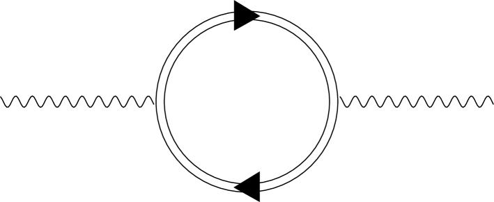
FIG. 1.: Vacuum polarization in a strong magnetic field. The double solid line denotes the electron propagator which includes all contributions of the vertices from the magnetic field.

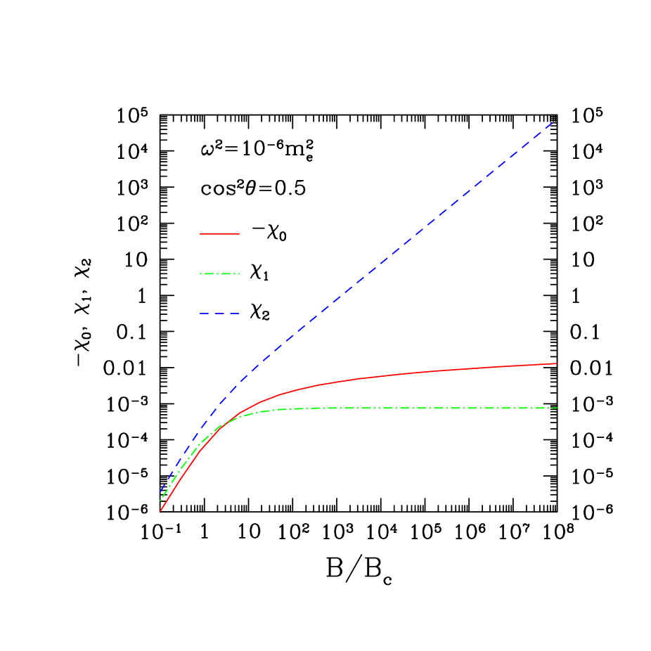
FIG. 2.: Plots of $-\chi_{0}$, $\chi_{1}$ and $\chi_{2}$ as a function of $B/B_{c}$. Here we adapt $\omega^{2}=10^{-6}m_{e}^{2}$ and $\cos^{2}\theta=0.5$. We find that the magnitude of $\chi_{0}$ increases as $B/B_{c}$ increases ($\propto\log(B/B_{c})$), $\chi_{1}$ reaches the limit value ($\sim$ 7.7 $\times 10^{-4}$), and $\chi_{2}\simeq\frac{e^{2}}{3\pi}B/B_{c}$ for $B/B_{c}\gg 1$.

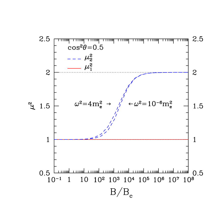
FIG. 3.: Plot of the refractive indices as a function of $B/B_{c}$. The solid line represents $\mu^{2}_{1}$ and the dashed line represents $\mu^{2}_{2}$. The left (right) dashed line is the case for $\omega^{2}=4m_{e}^{2}\ (10^{-6}m_{e}^{2})$. Here we adapt $\omega^{2}=10^{-6}m_{e}^{2}$ and $\cos^{2}\theta=0.5$. We find that $\mu^{2}_{2}$ reaches the limit value ($1/\cos^{2}\theta=2$) in the strong $B$ limit.

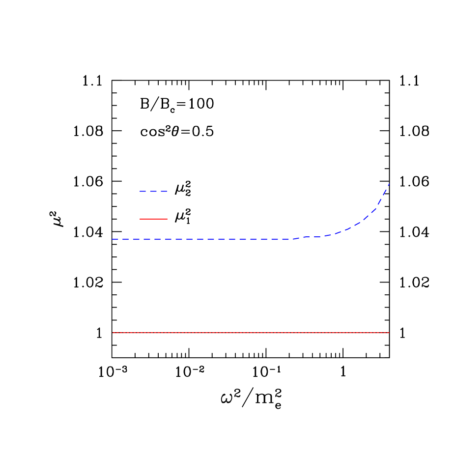
FIG. 4.: Plot of the refractive indices as a function of $\omega^{2}/m_{e}^{2}$. The solid line represents $\mu^{2}_{1}$ and the dashed line represents $\mu^{2}_{2}$. Here we adapt $B/B_{c}=10^{2}$ and $\cos^{2}\theta=0.5$.

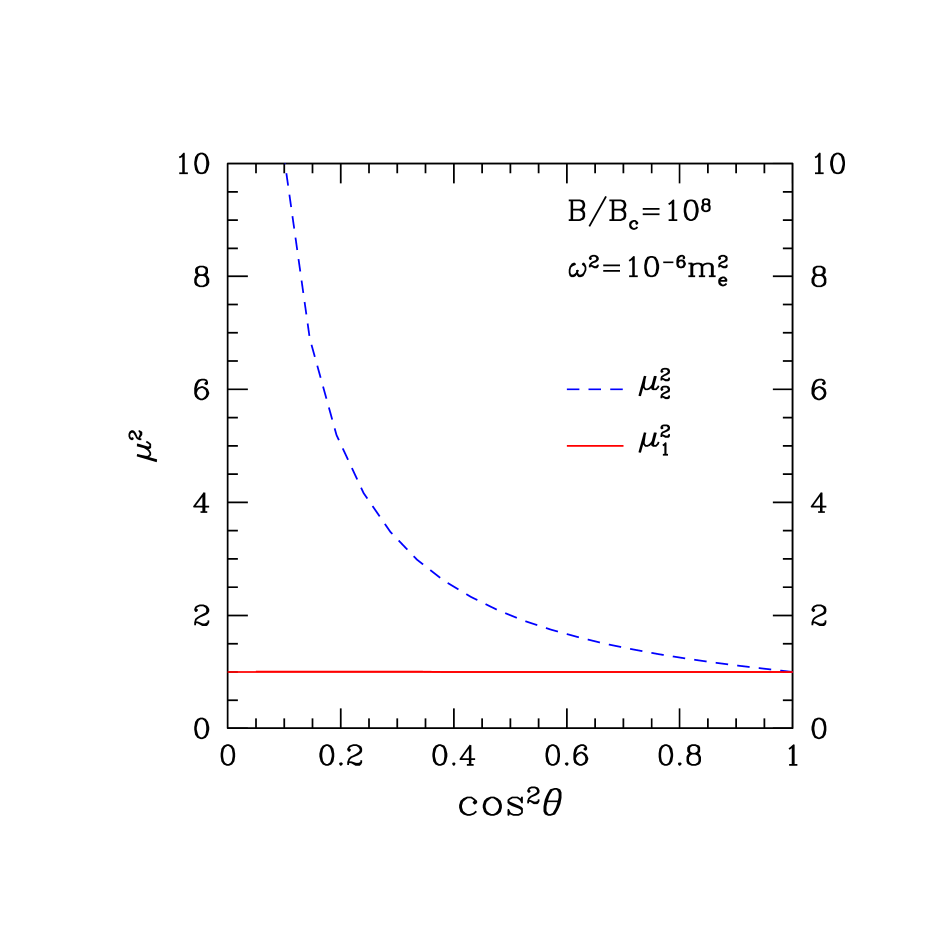
FIG. 5.: Plot of the refractive indices as a function of $\cos^{2}\theta$. The solid line represents $\mu^{2}_{1}$ and the dashed line represents $\mu^{2}_{2}$. Here we adapt $B/B_{c}=10^{8}$ and $\omega^{2}=10^{-6}m_{e}^{2}$. We find that $\mu_{2}^{2}$ scales $1/\cos^{2}\theta$ in such a strong $B$ limit.