Are Compact Hyperbolic Models Observationally Ruled Out?

Abstract

We revisit the observational constraints on compact(closed) hyperbolic(CH) models from cosmic microwave background(CMB). We carry out Bayesian analyses for CH models with volume comparable to the cube of the present curvature radius using the COBE-DMR data and show that a slight suppression in the large-angle temperature correlations owing to the non-trivial topology explains rather naturally the observed anomalously low quadrupole which is incompatible with the prediction of the standard infinite Friedmann-Robertson-Walker models. While most of positions and orientations are ruled out, the likelihoods of CH models are found to be much better than those of infinite counterparts for some specific positions and orientations of the observer, leading to less stringent constraints on the volume of the manifolds. Even if the spatial geometry is nearly flat as $\Omega_{tot}=0.9-0.95$, suppression of the angular power on large angular scales is still prominent for CH models with volume much less than the cube of the present curvature radius if the cosmological constant is dominant at present.

1 Introduction

In the framework of modern cosmology, one often takes it for granted that the spatial geometry of the universe with finite volume is limited to that of a 3-sphere. However, if we drop the assumption of simply connectivity of the spatial geometry, then flat and hyperbolic(constantly negatively curved) spaces can be closed as well. Therefore non-positive curvature of the spatial geometry does not necessarily implies the infinite space. For instance, the simplest example of a constantly curved finite-volume space with non-trivial topology is a flat 3-torus which can be obtained by identifying the opposite faces of a cube by translations in the Euclidean 3-space. Construction of compact(closed) hyperbolic(CH) spaces is somewhat complicated but one can systematically create a countably infinite number of topologically distinct classes of CH spaces by performing topological surgeries on a certain space. In order to avoid confusion, it might be better to call a cosmological model whose spatial geometry is described by a connected and simply connected constantly negatively curved space as an “infinite hyperbolic” model rather than an “open” model which has been commonly used in the literature of astrophysics.
Since 1993, a number of articles concerned with constraints on the topology of flat models with no cosmological constant using the COBE-DMR data have been published. [2, 3, 4, 5, 6] The large-angle temperature fluctuations in the cosmic microwave background(CMB) discovered by the COBE satellite constrain the topological identification scale $L$ larger than 0.4 times the diameter of the observable region; in other words, the maximum expected number $N$ of copies of the fundamental domain inside the last scattering surface in the comoving coordinates is $\!\sim$8 for compact flat models without the cosmological constant. Assuming that the primordial power spectrum is scale-invariant($n\!=\!1$) then the large-angle power is strongly suppressed since fluctuations on scales larger than the physical size of the spatial hypersurface are strongly suppressed.
In contrast, a large amount of large-angle fluctuations can be produced for compact low density models owing to the decay of gravitational potential near the present epoch which is known as the integrated Sachs-Wolfe effect.[8] If the spatial geometry is flat or hyperbolic then the physical distance between two separated points $P_{1}$ and $P_{2}$ which subtends a fixed angle at the observation point $O$ becomes larger as the distance from $O$ to $P_{1}$ or $P_{2}$ increases. Large-angle fluctuations can be generated at late epoch when the fluctuation scale “enters” the topological identification scale $L$. Recent statistical analyses using only the power spectrum have shown that the constraints on the topology are not stringent for small CH models including the smallest (Weeks) and the second smallest (Thurston) known manifolds and an non-arithmetic orbifold [9, 10, 11, 12] and also for a flat compact toroidal model with the cosmological constant.[13]
These results are clearly at odds with the previous constraints [14, 15] on CH models based on pixel-pixel correlation statistics. It has been claimed that the statistical analysis using only the power spectrum is not sufficient since it can describe only isotropic (statistically spherically symmetric) correlations. This is true inasmuch one considers fluctuations observed at a particular point. Because any CH spaces are globally anisotropic, expected fluctuations would be statistically globally anisotropic at a particular point.
However, in order to constrain CH models, it is also necessary to compare the expected fluctuation patterns observed at every place of the observer to the data since all CH spaces are globally inhomogeneous.[16] It should be emphasized that the constraints obtained in the previous analyses are only for CH models at a particular observation point $P$ where the injectivity radius is locally maximum for 24 particular orientations. $P$ is rather special one in the sense that some of the mode functions often (eigenfunctions of the Laplacian) have symmetric structure.[17] It is often the case that the base point $P$ becomes a fixed point of symmetries of the Dirichlet domain or of the space itself. At different places the statistically averaged temperature correlations significantly changes their anisotropic structure as implied by the random Gaussian behavior of the mode functions of the Laplace-Beltrami operator.[17] Thus it is of crucial importance to carry out Bayesian analyses incorporating the dependence of the statistically averaged correlations on the position of the observer.
On the other hand, recent CMB observations have succeeded in measuring the amplitude and the peak of the angular power spectrum on small angular scales. Assuming that initial fluctuations are purely adiabatic seeded by quantum fluctuations then the first acoustic peak at $l\sim 200$ implies nearly flat geometry.[18, 19] This seems to deny any spherical or hyperbolic models. However, if one considers generalized initial fluctuations that include isocurvature modes of baryons, cold dark matter and neutrinos, the uncertainty in estimating the curvature significantly increases.[20] In order to decrease the uncertainty in the cosmological parameters one needs information of polarization[20, 21] which will be supplied by the future satellite missions, namely MAP and Planck. Until then we should interpret the recent CMB observations as which implies “not grossly curved spatial geometry” rather than “rigorously flat geometry”.
Even if the spatial geometry is nearly flat, the effect of the non-trivial topology is still prominent provided that the spatial hypersurface is much smaller than the observable region at present. However, we cannot expect a very small CH space since there is a lower bound $V_{min}$ for the volume $V$ of CH spaces. The precise value of $V_{min}$ is not known but it has been proved that $V>0.1667R^{3}$ where $R$ denotes the curvature radius for CH manifolds. The smallest known example has been discovered by Weeks[22] which has volume $0.9427R^{3}$ called the Weeks manifold. If we allow CH orbifold models then the volume can be much smaller. For instance, the smallest known orbifold has volume $V=0.0391R^{3}$.
Suppose that the cosmological constant or the “missing energy” with negative equation-of-state dominates the present energy density as the recent observations of SNIa imply [23, 24] then the comoving radius of the last scattering surface in unit of curvature radius becomes large because of the slow decrease in the cosmic expansion rate in the past. For instance, the number $N$ of copies of the fundamental domain inside the last scattering in the comoving coordinates is approximately 17.2 for a Weeks model with $\Omega_{\Lambda}\!=\!0.65$ and $\Omega_{m}\!=0.2\!$ whereas $N\!=\!2.5$ if $\Omega_{\Lambda}\!=\!0$ and $\Omega_{m}\!=0.85\!$. $N$ can be much larger for small orbifold models. Thus, even in the case of nearly flat geometry, there are possibilities that we can observe the imprint of the non-trivial topology.
In this paper, we investigate the CMB anisotropy in CH models(manifold and orbifold) with small volume with or without the cosmological constant. In section 2 we briefly describe the necessary ingredients of the geometry and topology of CH spaces. In section 3 the time evolution of the scalar-type perturbation which can be used for simulating the CMB anisotropy is described. In section 4 we estimate the degree of suppression in the large-angle power for manifold and orbifold models. In section 5 we carry out Bayesian analyses using the COBE-DMR data. In the last section we summarize our results.

2 Compact Hyperbolic Spaces

The discrete subgroup $\Gamma$ of the orientation-preserving isometry group of the simply-connected hyperbolic 3-space $H^{3}$ (which is isomorphic to $PSL(2,\mathbb{C})$) is called the Kleinian group. Any orientable CH 3-spaces (either manifold or orbifold) can be described as compact quotients$M=H^{3}/\Gamma$. Let us represent $H^{3}$ as an upper half space ($x_{1},x_{2},x_{3}$) for which the metric is given by

$$ds^{2}=\frac{R^{2}(dx_{1}^{2}+dx_{2}^{2}+dx_{3}^{2})}{x_{3}^{2}},$$ (1)

where $R$ is the curvature radius. In what follows, $R$ is set to unity without loss of generality. If we represent a point $p$ on the upper-half space, as a quaternion whose fourth component equals zero, then the actions of $PSL(2,{\mathbb{C}})$ on $H^{3}\cup{\mathbb{C}}\cup\{\infty\}$ take the form

$$\gamma:p\rightarrow p^{\prime}=\frac{ap+b}{cp+d},~{}~{}~{}~{}~{}ad-bc=1,~{}~{}~{}p\equiv z+x_{3}{{\mathbf{j}}},~{}~{}~{}z=x_{1}+x_{2}{{\mathbf{i}}},$$ (2)

where a, b, c and d are complex numbers and $1$, ${\mathbf{i}}$ and ${\mathbf{j}}$ are the components of the basis of quaternions. The action $\gamma$ is explicitly written as

$$\gamma:H^{3}\cup{\mathbb{C}}\cup\{\infty\} \rightarrow H^{3}\cup{\mathbb{C}}\cup\{\infty\},$$

$$\gamma:(z(x_{1},x_{2}),x_{3})~{}~{} \rightarrow \Biggl{(}\frac{(az+b)(\overline{cz+d})+a\bar{c}x_{3}^{2}}{|cz+d|^{2}+|c|^{2}x_{3}^{2}},\frac{x_{3}}{|cz+d|^{2}+|c|^{2}x_{3}^{2}}\Biggr{)},$$ (3)

where a bar denotes a complex conjugate. Elements of $\Gamma$ for orientable CH manifolds are $SL(2,\mathbb{C})$ conjugate to

$$\pm\left(\begin{array}[]{@{\,}cc@{\,}}\exp({l/2+i\phi/2})&0\\ 0&\exp({-l/2-i\phi/2})\end{array}\right),~{}0<\phi\leq 2\pi,~{}l>0$$ (4)

which are called loxodromic if $\phi\neq 0$ and hyperbolic if $\phi=0$.
There are other classes of isometries of $H^{3}$ which have fixed points, namely, parabolic and elliptic elements. In matrix representation, they are $SL(2,\mathbb{C})$ conjugate to

$$\pm\left(\begin{array}[]{@{\,}cc@{\,}}1&1\\ 0&1\end{array}\right),~{}~{}\textit{parabolic}$$ (5)

and

$$\pm\left(\begin{array}[]{@{\,}cc@{\,}}\exp({i\phi/2})&0\\ 0&\exp({i\phi/2})\end{array}\right),~{}0<\phi\leq 2\pi,~{}~{}\textit{elliptic}$$ (6)

, respectively. An orientable CH orbifold can be realized as a compact quotient $H^{3}$ by $\Gamma$ which includes an elliptic element. If $\gamma$ includes a parabolic element, then the quotient space is called a cusped hyperbolic manifold. A cusp point corresponds to a fixed point at infinity by the parabolic transformation. In what follows we denote a “cusped manifold” as a finite-volume hyperbolic manifold with one cusp point or more.
Topological construction of CH spaces starts with a cusped manifold $M_{c}$. Let us first consider the two-dimensional case. If we glue two ideal hyperbolic triangles together on each sides, then we have a thrice punctured sphere. Because each side is isometric to a line, we can modify the gluing map by an arbitrary translation (in this case it is parametrized by ${{}\mathbb{R}}^{3}$). However, the obtained surface is not always complete. Let $h$ be a horocyclesegment, that is orthogonal to the two sides of the triangle centered at a vertex $v$. Extend $h$ counterclockwise about $v$ by horocycle segments that meet successive edges of ideal triangles. Finally it re-enters the orthogonal triangle as a horocycle concentric with $h$, at a distance $d(v)$. The obtained surface is complete if and only if $d(v)=0$ for all vertices $v$[25]. In this case, the condition $d(v)=0$ yields a hyperbolic manifold with three cusp points where the horocycles correspond to periodic geodesics associated with parabolic elements.

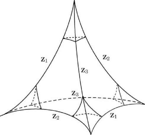
Figure 1: Parameterization of an ideal tetrahedron. Each edge $e$ is labelled with a complex number $z(e)$ and opposite edges have the same label. The four links (=Euclidean triangles realized as the intersections with horospheres in the neighborhood of vertices) are congruent each other. An ideal tetrahedron up to orientation-preserving similarity can be specified by one link which is parametrized by one of the $z(e)$.

Similarly, one can construct a cusped 3-manifold by gluing ideal polyhedra. Here we consider gluing of a set of $n$ ideal tetrahedra $T_{1},...,T_{n}$. $T_{i}$ is determined by the three dihedral angles $\alpha,\beta$ and $\gamma$ which satisfy $\alpha+\beta-\gamma=\pi$. Because the dihedral angles of opposite edges are equal, $T_{i}$ is essentially determined by two parameters. In order to represent the shape of an ideal tetrahedron $T_{i}$ , one can use the link $L(v)$ of a vertex $v$ at infinity which is an Euclidean triangle realized as the intersection of a horosphere with $T_{i}$ in the neighborhood of $v$. $L(v)$ can be described by two parameters and determines $T_{i}$ up to congruence. In order to parameterize $L(v)$, it is convenient to represent the Euclidean plane $E^{2}$ as $\mathbb{C}$.[25] To each vertex $v_{1}$ of a triangle ($v_{1},v_{2},v_{3}$) (the vertices are labeled in a clockwise order)in $\mathbb{C}$ we associate the ratio

$$z(v_{1})=\frac{v_{3}-v_{1}}{v_{2}-v_{1}}$$ (7)

of the sides adjacent to $v_{1}$. The ratios(with any starting point) should satisfy

$$z(v_{1})z(v_{2})z(v_{3}) = -1,$$

$$1-z(v_{1})+z(v_{1})z(v_{2}) = 0.$$ (8)

Thus any $z(v_{i})$ determines the other two $z(v_{j})$s. An ideal tetrahedron can be specified by any $z(v_{i})$ having two parameters up to orientation-preserving similarity (figure 1). The gluing conditions of ideal tetrahedra $T_{1},...,T_{n}$ are algebraically given by

$$z(e_{1})\cdot z(e_{2})\cdot\cdots\cdot z(e_{m}) = 1,$$

$$\textrm{arg}z(e_{1})+\cdots+\textrm{arg}z(e_{m}) = 2\pi,~{}0\leq\textrm{arg}\leq\pi$$ (9)

where $e_{i}$s are the edges of ideal tetrahedra. Note that even if the above conditions are satisfied the obtained manifold is sometimes incomplete where the developing image of $L(v)$ is ${\mathbb{C}}-0$ after an appropriate translation. If $L(v)$ properly tessellates ${\mathbb{C}}$ then the obtained manifold $M$ is complete and the boundary of the neighborhood of a vertex at infinity is either a torus or a Klein bottle. $M=M_{c}$ is topologically equivalent to the complement of a knot $K$ or link $L$(which consists of knots) in a 3-sphere $S^{3}$ or some other closed 3-space. A surgery in which one removes the tubular neighborhood $N$ of $K$ whose boundary is homeomorphic to a torus, and replace $N$ by a solid torus so that a meridian in the solid torus goes to $(p,q)$ curve on $N$ is called $(p,q)$ Dehn surgery. Except for a finite number of cases, Dehn surgeries on $K$ where $p$ and $q$ are co-prime always yield CH 3-manifolds which implies that most compact 3-manifolds are hyperbolic[26] since every closed 3-manifolds can be obtained by performing such Dehn surgeries. CH 3-orbifolds whose singular sets consist of lines can be obtained by $(p,q)$ Dehn surgeries where $p$ and $q$ are not co-prime.
The above procedure for obtaining CH 3-spaces is manifestly defined but somewhat complicated for computation by hand. A computer program “SnapPea” developed by Weeks[27] can numerically handle the procedure, namely computation of hyperbolic structure of cusped manifolds, performing various Dehn surgeries and so on. SnapPea can also compute the volume, fundamental group, homology, symmetry group, Chern-Simon invariant, length spectrum and other quantities.

Figure 2: The Dirichlet fundamental domains of the Weeks manifold (volume$=0.9427$)(left) and the smallest orbifold that is covered by the Weeks manifold (volume$=0.0786$)(right) viewed from opposite directions in the Klein(projective) coordinates. Colors on the faces represent the identification maps.

In contrast to compact flat spaces with no scale, there is a lower bound for the volume of CH 3-spaces. It has been proved that the volumes of CH 3-manifolds cannot be smaller than $0.16668\dots$[28] although no concrete example with such volume is known. The smallest known CH 3-manifold is called the Weeks manifold with volume $0.9427$ which can be obtained by a (3,-1) Dehn surgery on a cusped manifold $m003$ with volume 2.0299(one of the smallest known cusped manifold). Performing a (-2,3) Dehn surgery on m003 yields the second smallest known manifold called the Thurston manifold with volume $0.9814$. Except for a finite number of cases, Dehn surgeries on m003 yield CH manifolds with volume less than that of m003.[26] As $|p|$ and $|q|$ becomes large, the volume of the space converges to that of the original cusped manifold $M_{c}$. Therefore, for the purpose of classification of CH spaces it is better to exclude “almost non-compact” spaces that are very similar to $M_{c}$. The volume of CH 3-orbifolds can be much smaller since every CH 3-orbifold is covered by a CH 3-manifold(there are an infinite number of coverings). For instance, the smallest volume of a CH 3-orbifold whose finite-sheeted cover is the Weeks manifold is $V=0.9427/12=0.0786$ (see figure 2)since the isometry group of the Weeks manifold is $D6$(dihedral group), which does not have any fixed planes. The smallest known orientable 3-orbifold has volume $V=0.0391$ which also does not have any fixed planes.[29] A known lower bound for the volume of orientable orbifolds is $V>0.0000013$.[30]

3 CMB Anisotropy

In what follows we assume that the matter consists of two components:a relativistic and an non-relativistic one ($\Omega_{m}=\Omega_{r}+\Omega_{n}$). From the Friedmann equation, the integral representation for the time evolution of the scale factor $a$ (normalized to 1 at present time) in terms of the conformal time $\eta$ is given by

$$\eta(a)=R\int_{0}^{a}\frac{da}{\sqrt{\textrm{sign}K((\Omega_{n}a+\Omega_{r}+\Omega_{\Lambda}a^{4})/(\Omega_{m}+\Omega_{\Lambda}-1)-a^{2})}},K\neq 0,$$ (10)

where $R=|K|^{-1/2}$ is the curvature radius at present. The above presentations can also be written in terms of some special functions but they are too complex to describe here.
The scalar perturbation equations are exactly same as those without the cosmological constant. Let us consider the adiabatic case and assume that the anisotropic pressure is negligible. Then from the linear perturbation equation, the time evolution of the Newtonian curvature perturbation $\Phi$ of $k$ mode is given by, [31]

$$\Phi^{\prime\prime}+3{\cal{H}}(1+c_{s}^{2})\Phi^{\prime}+c_{s}^{2}k^{2}\Phi+(2{\cal{H}}^{\prime}+(1+3c_{s}^{2})({\cal{H}}^{2}-K))\Phi=0,$$ (11)

where ^′ denotes the conformal time derivative $d/d\eta$, ${\cal{H}}\equiv a^{\prime}/a$, G is the Newton’s constant, $c_{s}$ is the sound speed of the fluid which is explicitly written in terms of the density of relativistic matter $\rho_{r}$ and non-relativistic matter $\rho_{m}$

$$c_{s}^{2}=\frac{1}{3}\frac{\rho_{r}}{\rho_{r}+\frac{3}{4}\rho_{m}}.$$ (12)

Let us consider the early universe when the radiation is dominant and the effect of the curvature and the cosmological constant is negligible. Then (10) yield the evolution of the scale factor as $a\propto\eta$ and (11) is reduced to

$$\Phi^{\prime\prime}+\frac{4}{\eta}\Phi^{\prime}+\frac{k^{2}}{3}\Phi=0,$$ (13)

which has an analytic solution

$$\Phi(\eta)=\eta^{-3}\{(\omega\eta\cos(\omega\eta)-\sin(\omega\eta))C_{1}+(\omega\eta\sin(\omega\eta)-\cos(\omega\eta))C_{2}\},$$ (14)

where $\omega=k/\sqrt{3}$ and $C_{1}$ and $C_{2}$ are constants which depend on $k$.[31] Around $\eta=0$, (14) can be expanded as

$$\Phi(\eta)=\eta^{-3}\{C_{2}+\frac{C_{2}}{2}\omega^{2}\eta^{2}-\frac{C_{1}}{3}\omega^{3}\eta^{3}-\frac{C_{2}}{8}\omega^{4}\eta^{4}+{\cal O}((\omega\eta)^{5})\}.$$ (15)

Thus for the long-wavelength modes($\omega\eta<<1$), the non-decaying mode ($C_{2}=0$) has constant amplitude and the time derivative at the initial time vanishes,

$$\Phi\sim\textrm{const},~{}~{}~{}~{}~{}\Phi^{\prime}(0)=0.$$ (16)

During the radiation-matter equality time the equation of state change from $w=1/3$ to $w=0$. Then the amplitude of long-wavelength modes changes by a factor of $9/10$. In the curvature or $\Lambda$ dominant epoch the amplitude decays as $1/a$.
Assuming that the matter is dominant at the last scattering and the anisotropic pressure is negligible, the temperature fluctuation on large angular scales can be written in terms of the Newtonian curvature perturbation $\Phi$ as

$$\frac{\Delta T}{T}({\mathbf{n}})=-\frac{1}{3}\Phi(\eta_{\ast},(\eta_{0}-\eta_{\ast}){\mathbf{n}})-2\int_{\eta_{\ast}}^{\eta_{0}}\frac{\partial\Phi(\eta,(\eta_{0}-\eta){\mathbf{n}})}{\partial\eta}d\eta,$$ (17)

where ${\mathbf{n}}$ denotes the unit vector which points the sky and $\eta_{\ast}$ and $\eta_{0}$ correspond to the last scattering conformal time and the present conformal time, respectively.[32, 33] The first term in the right-hand side in (17) describes the ordinary Sachs-Wolfe (OSW) effect while the second term describes the integrated Sachs-Wolfe (ISW) effect.

4 Angular power spectra

In order to analyze the temperature anisotropy in the sky it is convenient to expand it in terms of spherical harmonics $Y_{lm}$ as

$$\frac{\Delta T}{T}({\mathbf{n}})=\sum_{lm}a_{lm}Y_{lm}({\mathbf{n}}),$$ (18)

where ${\mathbf{n}}$ is the unit vector along the line of sight. Because each mode of scalar perturbation evolves independently in the locally isotropic and homogeneous background space, we need only the information of eigenmodes $u_{\nu}$ of the Laplace-Beltrami operator $\Delta$ in the CH space (i.e. elements of an orthonormal basis of $L^{2}(H^{3}/\Gamma)$) which can be expanded in terms of eigenmodes in the simply connected infinite hyperbolic space in the spherical coordinates ($\chi,\theta,\phi$) as

$$u_{\nu} = \sum_{lm}\xi_{\nu lm}\,X_{\nu l}(\chi)Y_{lm}(\theta,\phi),$$

$$X_{\nu l}(\chi) = \frac{\Gamma(l+1+\nu i)}{\Gamma(\nu i)}\sqrt{\frac{1}{\sinh\chi}}P^{-l-1/2}_{\nu i-1/2}(\cosh\chi),$$ (19)

where $~{}\nu^{2}=k^{2}-1$, $Y_{lm}$ denotes (complex) spherical harmonics, $P$ is the associated Legendre function and $\xi_{\nu lm}$ represents the expansion coefficients.
Assuming that the initial fluctuations obey the Gaussian statistic, and neglecting the tensor-type perturbations and anisotropic pressure and matter is dominant at the last scattering epoch, the angular power spectrum $C_{l}=<|a_{lm}|^{2}>$ ($<>$ denotes an ensemble average over the initial perturbation) for CH models can be written as

$$(2\,l+1)\,C_{l} = \sum_{\nu,m}\frac{4\pi^{4}~{}{\cal P}_{\Phi}(\nu)}{\nu(\nu^{2}+1)V(M)}~{}|\xi_{\nu lm}|^{2}|F_{\nu l}|^{2},$$

$$F_{\nu l}(\eta_{o})\!\! \equiv \!\!\frac{1}{3}\Phi_{t}(\eta_{\ast})X_{\nu l}(\eta_{o}\!-\!\eta_{\ast})\!+\!\!2\!\!\int_{\eta_{\ast}}^{\eta_{o}}\!\!\!\!\!\!d\eta\,\frac{d\Phi_{t}}{d\eta}X_{\nu l}(\eta_{o}\!-\!\eta),$$ (20)

where $\nu\!=\!\sqrt{k^{2}-1}$, ${\cal P}_{\Phi}(\nu)$ is the initial power spectrum, and $\eta_{\ast}$ and $\eta_{o}$ are the last scattering and the present conformal time, respectively. $\Phi_{t}=\Phi/\Phi(0)$ and $V(M)$ is the comoving volume of the space. The (extended) Harrison-Zel’dovich spectrum corresponds to ${\cal P}_{\Phi}(\nu)\!=\!Const.$ which we shall use as the initial condition. It should be noted that $C_{l}$’s depend on the position and orientation of the observer since CH spaces are globally inhomogeneous. Therefore, it is better to consider the ensemble average $\hat{C}_{l}\equiv<C_{l}>$ taken over the position of the observer. Using Weyl’s asymptotic formula one can easily show that $\hat{C}_{l}$’s coincide with those for the infinite counterpart in the limit $\nu\rightarrow\infty$ provided that $<|\xi_{\nu lm}|^{2}>\propto\nu^{-2}$. Thus all we have to do is to numerically compute the expansion coefficients $\xi_{\nu lm}$ which contain the information of global topology and geometry.
In order to estimate the suppression in the angular power $\hat{C}_{l}$ it is convenient to write $\hat{C}_{l}$ in terms of the transfer function $T_{l}(k)$ which satisfies [36]

$$\frac{2l+1}{4\pi}\tilde{C}_{l}=\int T_{l}^{2}(k){\cal P}(k)\frac{dk}{k},$$ (21)

where $\tilde{C}_{l}$ denotes the angular power for the infinite counterpart. For CH models, $\hat{C}_{l}$ is written as a sum of $T_{l}^{2}(k)$ for discrete wave numbers $k_{i}$.
On large angular scales, the behavior of the angular power $\hat{C}_{l}$ is determined by low-lying modes which are susceptible to the global topology of the background geometry since the amplitude of each mode is proportional to $\sim\nu^{-5}|F_{\nu l}|^{2}$. As shown in figure 3, one can see that the transfer function corresponding to the first eigenmode $T_{l}^{2}(k_{1})$ mimics the angular dependence of $\hat{C}_{l}$.
The large-angle power owing to the OSW effect suffers a significant suppression since fluctuations on scales beyond the actual size of the space are not allowed. The angular cutoff scale $l_{cut}$ above which the OSW contribution suffers a suppression corresponds to the angular scale of the first eigenmode on the last scattering surface, which can be written in terms of the comoving volume $V(M)$ and the smallest non-zero wavenumber $k_{1}$ as [35]

$$l_{cut}=\frac{k_{1}}{4}\sqrt{V^{-1}((\sinh(2(R_{LSS}+r_{ave}))-\sinh(2(R_{LSS}-r_{ave}))-4r_{ave}))},$$ (22)

where $V=\pi(\sinh(2r_{ave})-2r_{ave})$ and $R_{LSS}$ denotes the comoving radius of the last scattering surface. For the Weeks models ($V=0.94$ and $k_{1}=5.27$), $l_{cut}=26$ for $\Omega_{0}=0.2$ and $l_{cut}=7$ for $\Omega_{0}=0.6$.

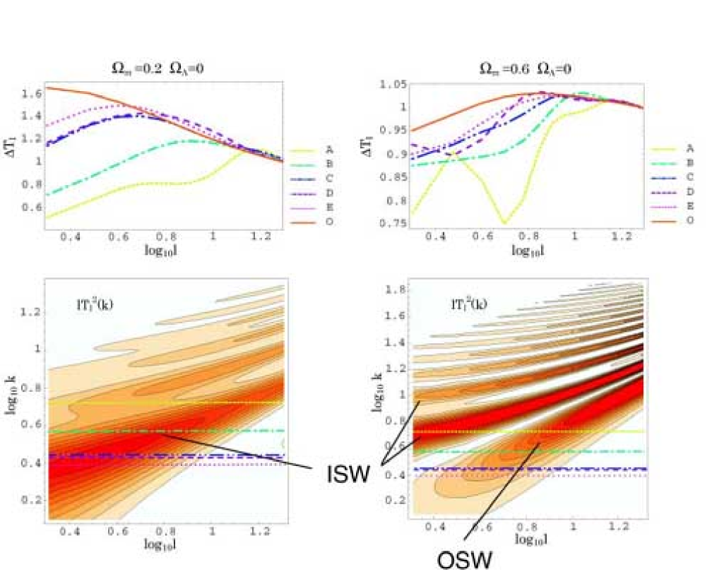
Figure 3: Suppression in the large-angle power $\Delta T_{l}\equiv\sqrt{l(l+1)\hat{C}_{l}/(2\pi)}$ for 5 CH models (name,volume)= A:(m003(3,-1)(Weeks),0.94), B:(m010(-1,3),1.9), C:(m082(-2,3),2.9), D:(m288(-5,1),3.9) E:(s873(-4,1), 4.9) in comparison with the one for the infinite hyperbolic model(denoted as O). All the plotted values are normalized by $\Delta T_{20}$ for the infinite hyperbolic model. The $l$ dependence of $\Delta T_{l}$ can be approximately given by the transfer function $lT^{2}_{l}(k_{1})$. First eigenvalues $k_{1}$ for the five models are represented as horizontal lines in lower figures. The unit of $k$ is equal to the inverse of the present curvature radius.

From figure 3 one can see that the angular scales $l_{cut}$ corresponding to the intersection of $k=k_{1}$ and the OSW ridge of the transfer function well agree with these analytic estimates. On smaller angular scales $l>>l_{cut}$, the powers asymptotically converge to those for the infinite counterpart.
Because the large-angle power in the COBE-DMR data is nearly flat, it seems that the suppression leads to a bad fit to the data on large angular scales. However, for low density models we should consider the ISW effect owing to the gravitational potential decay at the curvature dominant epoch $1+z\sim(1-\Omega_{0})/\Omega_{0}$ or $\Lambda$ dominant epoch $1+z\sim(\Omega_{\Lambda}/\Omega_{0})^{1/3}$ well after the last scattering time. For a given angular scale $l$ the comoving scale $k^{-1}$ of a fluctuation that is produced at late time is decreased. On the other hand, fluctuations do not suffer suppression if the comoving scales of fluctuations are sufficiently smaller than the actual size of the space $k^{-1}<<r_{ave}$. Therefore, the suppression on the ISW contribution is less stringent compared with the OSW contribution. Interestingly, the suppression on the angular power owing to the mode-cutoff reduces the excess power owing to the ISW effect, resulting in a nearly flat power with a slight suppression on large angular scales $2\leq l\leq 10$.
The suppression of the power is crudely estimated by the number $N$ of the copies of the fundamental domain inside the last scattering surface in comoving coordinates. Suppose that $\Omega_{\Lambda}\!=\!0$. Then the comoving radius of the last scattering surface in terms of the present curvature radius $R$

$$R_{LSS}\approx R\cosh^{-1}(2/\Omega_{m}-1),$$ (23)

gives the comoving volume $v_{LSS}$ of the ball inside the last scattering surface

$$v_{LSS}\approx\pi R^{3}(\sinh(2R_{LSS}/R)-2R_{LSS}/R).$$ (24)

For example, $v_{LSS}\!\sim\!490R^{3}$ for $(\Omega_{m},\Omega_{\Lambda})\!=\!(0.2,0)$ whereas $v_{LSS}\!\sim\!R^{3}$ for $(\Omega_{m},\Omega_{\Lambda})\!=\!(0.9,0)$. Thus in nearly flat models, the imprint of the non-trivial topology is prominent only for the case where the volume is smaller than $R^{3}$. However, if one includes the cosmological constant then $R_{LSS}$ (in unit of $R$) becomes large because of a slow increase in the cosmic expansion rate in the past. For instance, $N=8.7$ for a Weeks model (the smallest known manifold) with $\Omega_{\Lambda}\!=\!0.7$ and $\Omega_{m}\!=0.2\!$ whereas $N\!=\!1.2$ for $\Omega_{\Lambda}\!=\!0$ and $\Omega_{m}\!=0.9\!$. Furthermore, if one allows orbifold models, $N$ can be much larger than these values. For instance, $N=51.8$ for the smallest orbifold (volume$=0.0391R^{3}$) with $\Omega_{\Lambda}\!=\!0.7$ and $\Omega_{m}\!=0.25\!$.

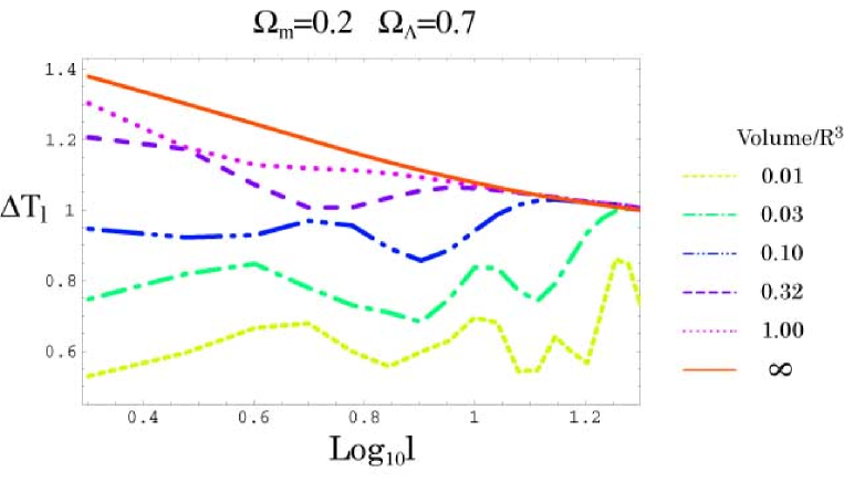
Figure 4: Suppression in large-angle power $\Delta T_{l}=\sqrt{l(l+1)\hat{C}_{l}/2\pi}$ for small (hypothetical) orbifold models with $\Omega_{m}=0.2$ and $\Omega_{\Lambda}=0.7$ in comparison with the infinite hyperbolic model with the same density parameters. The amplitude is normalized by $\Delta T_{20}$ for the infinite hyperbolic model.

Now let us consider the angular power spectrum for orbifold models. Assuming no very short periodic geodesics and no supercurvature modes, one can crudely estimate the low-lying eigenvalues [35] from the asymptotic form of the number function(spectral staircase) [37]

$$n(E)=\frac{V(M)}{6\pi^{2}}\nu^{3}+c_{2}\nu^{2}+c_{1}\nu+c_{0}+O(e^{-\pi\nu/5}),~{}\nu^{2}=E-1,$$ (25)

where $n(E)$ denotes the number of eigenvalues of the Laplace-Beltrami operator equal to or less than $E$ and $c_{i}$’s are the constants determined from the plane reflection, elliptic and inverse elliptic elements of the discrete isometry group and the area of the fixed planes. For orientable orbifolds with only fixed lines, the constants vanish except for $c_{1}$ which is written in terms of elliptic elements. If we consider only such orbifolds with small volume (large $\nu_{1}$) then the dominant contribution comes from the first term in the right hand side in (25). If we further assume that the eigenmodes have the same pseudo-random property as those of CH manifolds[38] then we can readily estimate the angular powers. As shown in figure 4 the suppression of the large-angle power for small orbifold models is still prominent in the case of nearly flat geometry.

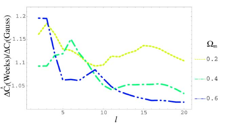
Figure 5: Fractional uncertainty in the angular power $\Delta\hat{C}_{l}=(\textrm{Var}(\hat{C}_{l}))^{1/2}/<\hat{C}_{l}>$ for the Weeks models relative to the values for the Gaussian models $\Delta C_{l}(\textrm{Gauss})=(\textrm{Var}(C_{l}))^{1/2}/<C_{l}>=(2/2l+1)^{1/2}$

Another feature of the non-trivial topology is an increase in the cosmic variance which is attributed to the global inhomogeneity and anisotropy of the background geometry. If we assume the pseudo-random Gaussianity of the expansion coefficients $\xi_{\nu lm}$ as observed in the smallest CH manifolds[34, 17] then uncertainty in the power (which may be called the geometric variance) can be easily estimated. For CH models, $a_{lm}$ is given by a sum of products of the initial perturbation $\Phi_{\nu}(0)$ times the expansion coefficients

$$a_{lm}=\sum_{\nu}\Phi_{\nu}(0)\xi_{\nu lm}F_{\nu l}.$$ (26)

If we fix the values of the primordial fluctuations then $a_{lm}$’s behave as if they are random Gaussian numbers and the angular power obeys the $\chi^{2}$ distribution. Because the degree of freedom ($k,m$) in the sum is always larger than $2l+1$, the geometric variance should be always smaller than the “initial variance” owing to the uncertainty in the initial conditions. Therefore, we expect that the net cosmic variance ($\approx$initial variance $+$ geometric variance) is not significantly greater than the values for the infinite counterpart.
In order to confirm the validity of the Gaussian assumption for computing the cosmic variance, firstly, we have compared the fractional uncertainty in the angular power $(2\leq l\leq 20)$ of the Weeks models using only the lowest 33 numerically computed eigenmodes ($k<13$) to those using the Gaussian random approximation for the expansion coefficients (corresponding to the same eigenvalues). It has turned out that the errors lie within several per cent for models with $\Omega_{m}=0.2,0.4$ and $0.6$(the relative errors are $0.08$ for $l=2$ and $<0.04$ for $l>2$).
Next, taking the contribution of higher modes into account, we have computed the fractional uncertainty in the angular power, which can be estimated by using the Gaussian approximation for the expansion coefficients (corresponding to the computed eigenvalues for $k<13$ and the approximated eigenvalues obtained from Weyl’s asymptotic formula for $k<60$) for the same parameters and we have compared the values with those using only the lowest 33 eigenmodes ($k<13$) and it has found that the errors lie within several per cent(however, for high matter density models the systematic increase in the variance owing to the artificial mode cut-off is much significant as the number of modes that contribute to the sum grows). As shown in figure 5, on large angular scales the fractional uncertainty in the angular power (for the Weeks models) with low matter density increases just 5 to 20 percent relative to the one for the Gaussian models. Thus the previous claim that the $C_{l}$’s have large cosmic variances[15] is not correct. On small angular scales, an increase in the number of eigenmodes that contributes to the power leads to a decrease in the geometric variance. Consequently, the cosmic variance converges to the one for the Gaussian model as implied by the central limit theorem.

5 Bayesian analysis

In this section, we study the likelihoods of CH models using the COBE data. Although here we only study manifold models, we expect the result for orbifold models (with the same volume) will not grossly change since the statistical property of eigenmodes are expected to be similar with those of manifolds[11].
The covariance in the temperature at pixel $i$ and pixel $j$ in the sky map is given by

$$M_{ij}=<T_{i}T_{j}>=\sum_{l}<a_{lm}a_{l^{\prime}m^{\prime}}>W_{l}W_{l}^{\prime}Y_{lm}(\hat{n_{i}})Y_{l^{\prime}m^{\prime}}(\hat{n_{j}})+<N_{i}N_{j}>,$$ (27)

where $<>$ denotes an ensemble average taken over all initial conditions, positions and orientations of the observer, $T_{i}$ represents the temperature in pixel $i$, $W_{l}^{2}$ is the experimental window function that includes effects of beam-smoothing and finite pixel size, $\hat{n_{i}}$ is the unit vector towards the center of pixel $i$ and $<N_{i}N_{j}>$ is the noise covariance between pixel $i$ and pixel $j$. If the fluctuations in the sky form an isotropic Gaussian field then the covariance is written as

$$M_{ij}=\frac{1}{4\pi}\sum_{l}(2l+1)W_{l}^{2}C_{l}P_{l}(\hat{n_{i}}\cdot\hat{n_{j}})+<N_{i}N_{j}>,$$ (28)

where $P_{l}$ is the Legendre function. Assuming a uniform prior distribution for a set of cosmological parameters, the probability distribution function of a power spectrum $C_{l}$ is given by

$$\Lambda(C_{l}|\vec{T})\propto\frac{1}{\det^{1/2}M(C_{l})}\exp\Biggl{(}\frac{1}{2}\vec{T}^{T}\cdot M^{-1}(C_{l})\cdot\vec{T}\Biggr{)},$$ (29)

where $\vec{T}$ denotes an array of the data of the temperature at pixels.
In the following analysis, we use the inverse-noise-variance-weighted average map of the 53A,53B,90A and 90B COBE-DMR channels. To remove the emission from the galactic plane, we use the extended galactic cut (in galactic coordinates).[39] After the galactic cut, best-fit monopole and dipole are removed using the least-square method. To achieve efficient analysis in computation, we further compress the data at “resolution 6” $(2.6^{o})^{2}$ pixels into one at “resolution 5” $(5.2^{o})^{2}$ pixels for which there are 1536 pixels in the celestial sphere and 924 pixels surviving the extended galactic cut. The window function is given by $W_{l}=G_{l}F_{l}$ where $F_{l}$ are the Legendre coefficients for the DMR beam pattern[40] and $G_{l}$ are the Legendre coefficients for a circular top-hat function with area equal to the pixel area which account for the pixel smoothing effect (the effect of the finite pixel size is non-negligible since the COBE-DMR beam FWHM is comparable to the size of “resolution 5” pixels).[41] To account for the fact that we do not have useful information about the monopole and dipole anisotropy, we set $C_{0}=C_{1}=100mK^{2}$ which renders the likelihood insensitive to monopole and dipole moments of several $mK$. We also assume that the noise in the pixels is uncorrelated which is found to be a good approximation.[42]
First of all, we set the initial condition as $\Phi^{2}_{\nu}(0)\!\propto\!1/(\nu(\nu^{2}+1))$ in order to approximately estimate the effect of the suppression in the large-angle power owing to the non-trivial topology (here we do not consider $\Phi_{\nu}(0)$ as random numbers). Then the fluctuations form a pseudo-Gaussian random field assuming pseudo-Gaussianity of the eigenmodes.

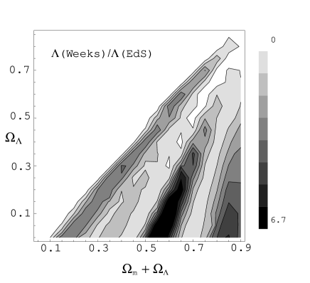
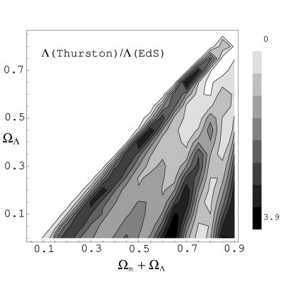
Figure 6: Plots of the ratio of likelihoods (assuming that the initial condition is fixed) for two smallest CH models (Weeks and Thurston) to a likelihood for the Einstein-de Sitter model ($\Omega_{m}=1.0$) with scale invariant initial spectrum ($n\!=\!1$). All the likelihoods are marginalized over the normalization of the power. Here we have assumed $\Phi^{2}_{\nu}(0)\!\propto\!1/(\nu(\nu^{2}+1))$ for CH models.

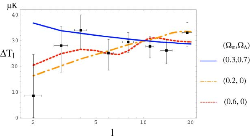
Figure 7: Plots of angular power spectrum $\Delta T_{l}=(l(l+1)\hat{C}_{l}/2\pi)^{1/2}$ of the COBE-DMR data (box) [43] in comparison with those for the Thurston models with $\Omega_{m}=0.2,0.6$ and a flat $\Lambda$ model with $\Omega_{m}=0.3$ and $\Omega_{\Lambda}=0.7$.

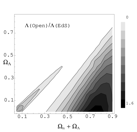
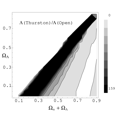
Figure 8: Plots of the ratio of likelihoods for the infinite hyperbolic “open” models ($n\!=\!1$) to one for the Einstein-de Sitter model ($n\!=\!1$) (left) and likelihoods for the Thurston models relative to one for infinite hyperbolic models (right). All the likelihoods are marginalized over the normalization of the power. Here we have assumed $\Phi^{2}_{\nu}(0)\!\propto\!1/(\nu(\nu^{2}+1))$ for the Thurston models. The slight improvement in the likelihood of infinite hyperbolic models with $\Omega_{m}<0.1$ is caused by the absence of the supercurvature modes. For the Thurston models with $\Omega_{m}=0.1\sim 0.3$ the likelihoods are significantly improved.

As shown in figure 6 for a wide range of parameters ($\Omega_{m}+\Omega_{\Lambda}>0.1$) the likelihoods for the smallest CH manifold models (Weeks and Thurston) are better than one for the Einstein-de Sitter model with scale-invariant spectrum ($n=1$) where $\Delta T_{l}=(l(l+1)C_{l}/2\pi)^{1/2}$ is almost constant in $l$. One can see the better fits to the COBE data for three parameter regions:1. $\Omega_{m}=0.5\sim 0.7$ with small $\Omega_{\Lambda}$ for which the angular power is peaked at $l\sim 4$ which corresponds to the first ISW ridge of the transfer function; 2. $\Omega_{m}=0.85\sim 0.9$ where the angular scale $l\sim 4$ which corresponds to the SW ridge;3. $\Omega_{m}\sim 0.2$ where the slope of the power on large angular scales $l<10$ fits well with the data.
For low matter density models with infinite volume(that is simply connected) the ISW effect leads to an excess power on large angular scales. Therefore the fit to the COBE data is not good because of the low quadrapole moment in the data(figure 7). In contrast, for small CH models, as we have seen, the excess power owing to the ISW effect is mitigated by a suppression owing to the mode-cutoff of the eigenmodes. Therefore, likelihoods for small CH models with low matter density are significantly improved compared with the infinite counterparts (figure 8). As the volume increases the likelihoods converge to those of the infinite counterparts although the convergence rate depends on cosmological parameters. One can see in figure 9 that the conspicuous difference for $\Omega_{m}\!=\!0.1-0.3$ still persists for volume$\sim 6$ whereas such difference is not observed for nearly flat cases ($\Omega_{tot}\!=\!\Omega_{m}+\Omega_{\Lambda}\!=\!0.9$). Roughly speaking, the difference in the power depends on the number $N$ of the copies of the fundamental domain inside the observable region at present.

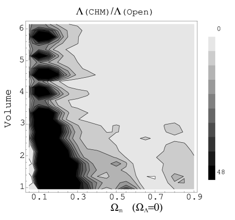
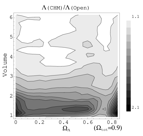
Figure 9: Plots of the ratio of approximated likelihoods for 27 CH models with volume ($0.94-6.15$) to a likelihood for the infinite hyperbolic counterparts. All the likelihoods are marginalized over the normalization of the power. Here we have assumed $\Phi^{2}_{\nu}(0)\!\propto\!1/(\nu(\nu^{2}+1))$ for CH models.

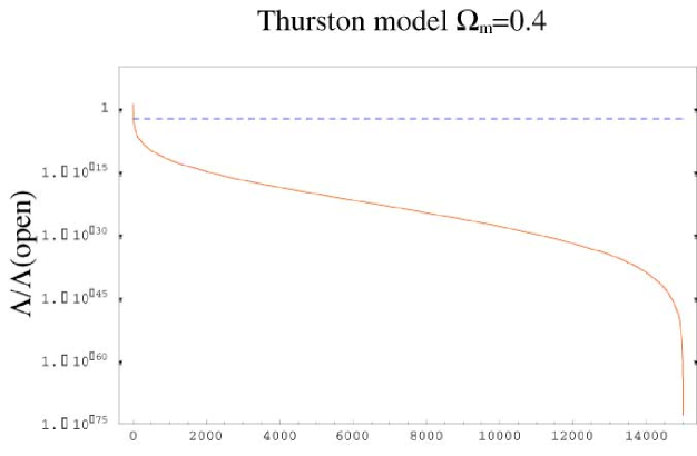
Figure 10: Plots of the ratio of “rigorous” likelihoods incorporating the effect of inhomogeneity and anisotropy of the background geometry for two compact multiply connected models relative to one for the infinite counterparts in ascending order(full curve) for 2000 random realizations of orientation for a closed flat toroidal (where the Dirichlet fundamental domain is a cube with sides $L=2.0H_{0}^{-1}$) model with $\Omega_{m}=0.1,\Omega_{\Lambda}=0.9$ (top) and for 1500 random realizations of position and 10 realizations of orientation for a Thurston model with $\Omega_{m}=0.4$ (bottom). The dashed lines denote the ensemble averaged values. The number $N$ of the copies of fundamental domain inside the observable region is 64.7 for the compact flat toroidal model and 72.3 for the Thurston model.

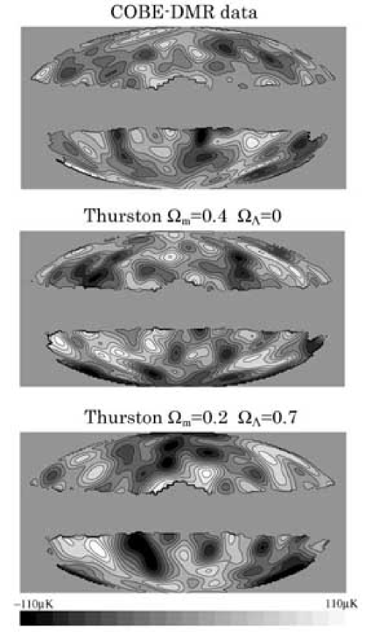
Figure 11: The top map shows the inverse-noise-variance-weighted averaged map of the COBE-DMR data at 53GHz and 90GHz after Wiener filtering assuming an angular power spectrum (averaged over the position of the observer) for a Thurston model with $\Omega_{m}=0.4$. Each of the mid and the bottom map shows a random realization of the CMB anisotropy (convolved with the COBE-DMR beam) at a position that gives a best-fit to the COBE-DMR data. For all the maps the “extended galactic cut” proposed by the COBE-DMR team was used and both the monopole and dipole were removed.

Next, we consider the effect of the non-diagonal elements which we have neglected so far. The likelihood for a homogeneous and isotropic ensemble is obtained by marginalizing the likelihoods all over the positions ${\mathbf{x}}_{obs}$ and the orientations $\alpha$ of the observer,

$$\Lambda=\int\!\!\sqrt{g}~{}d{\mathbf{x}}_{obs}d\alpha\Lambda({\mathbf{x}}_{obs},\alpha),$$ (30)

where we assume a constant distribution for the volume elements $\sqrt{g}d{\mathbf{x}}_{obs}$ and $d\alpha$ of a Lie group $SO(3)$ with a Haar measure. Assuming that the initial fluctuations are Gaussian with Harrison-Zel’dovich spectrum ($n=1$), the likelihood $\Lambda({\mathbf{x}}_{obs},\alpha))$ is given by (28) and (29) where $<a_{lm}a_{l^{\prime}m^{\prime}}>$ is written as

$$<a_{lm}a_{l^{\prime}m^{\prime}}>\propto\frac{1}{\nu(\nu^{2}+1)}\xi_{\nu lm}\xi_{\nu l^{\prime}m^{\prime}}F_{\nu l}F_{\nu l^{\prime}},$$ (31)

where $<>$ denotes an ensemble average taken over the initial condition and $F_{\nu l}$ describes contribution from the OSW effect and the ISW effect, respectively. Note that $\xi_{\nu lm}$’s are functions of ${\mathbf{x}}_{obs}$ and $\alpha$. In order to compute likelihoods, we use a compressed data at “resolution 3”$(20.4^{o})^{2}$ pixels in galactic coordinates for which there are 60 pixels surviving the extended galactic cut for efficient analysis in computation. Although the information of fluctuations on small angular scales $l>10$ is lost, we expect that they still provide us sufficient information for discriminating the effect of the non-trivial topology which is manifest on large-angular scales.
For the Thurston model, it has turned out that only 0.09 percent of the total of 1500 positions with 10 orientations are larger than the mean value. We have also computed likelihoods for 5100 positions with 40 orientations. Then the percentage has reduced to 0.02 from 0.09. The ratio of the likelihood marginalized over 5100 positions and 40 orientations to the likelihood of the infinite hyperbolic model with $\Omega_{m}\!=\!0.4$ is $\textrm{Log}_{10}(\Lambda/\Lambda(\textrm{open}))=-1.4$ and the maximum value is $\textrm{Log}_{10}(\Lambda(\max)/\Lambda(\textrm{open}))=3.6$. For 17 cases out of 204000 realizations, the likelihoods are much better than one for the infinite counterpart. Although 99.98 percent choices of position and orientation are ruled out, the likelihood for the remaining choices is approximately 4000 times larger than that for the infinite counterpart which boosts the probability of having skymaps consistent with the data. It has turned out that the positions that give a better fit to the data are scattered in the manifold and do not coincide with the point where the injectivity radius is locally maximal(=the center of the Dirichlet domain). This suggests that we are accidentally put at a certain place with a certain orientation. In other words, the observed sky gives us partial information about the position and orientation of the observer in the manifold although it is not enough to determine the values uniquely. The best-fit quadrupole normalization is $Q=(5C_{2}/4\pi)^{1/2}=0.022\pm 0.0024mK$ for 50 choices of position and orientation of the observer that satisfy $\Lambda/\Lambda(\textrm{open})>0.03$ while $Q=0.027\pm 0.0052mK$ for a total of 15000 realizations. For “bad” choices the best-fit normalization is somewhat high since it gives a large cosmic variance whereas the normalization is much lowered for “good” choices. One can see in figure 11 that a random realization of the skymap for the Thurston models does not appear grossly inconsistent with the COBE-DMR data. It turns out that the statistically averaged anisotropic correlation pattern depends sensitively on the position of the observer.
The likelihood analyses in [14, 15] are based on correlations for a particular choice of position $P$ where the injectivity radius is locally maximal with 24 orientations. It should be emphasized that the choice of $P$ as an observing point is very special one. For instance it is the center of tetrahedral and Z2 symmetry of the Dirichlet domain of the Thurston manifold although they are not belonging to the symmetry of the manifold.[17] In mathematical literature it is standard to choose $P$ as the base point which belongs to a “thick” part of the manifold since one can expect many symmetries. However, considering such a special point as the place of the observer cannot be verified since it is inconsistent with the Copernican principle. Because any CH models are globally inhomogeneous, one should compare fluctuation patterns expected at every place with every orientation.
To see the influence of global inhomogeneity, it is illustrative to compare the relative likelihoods(to the infinite counterpart) of the Thurston model with those of compact flat toroidal model (obtained by gluing opposite faces of a cube by three translations) which is globally homogeneous (i.e. every action of the discrete isometry group is a Clifford transformation). As shown in figure 10, for the toroidal model(that has approximately the same proportion to the currently observable region in size in comparison with the Thurston model), dependency on choices of position of the observer is less significant. Therefore one does not need a number of realizations for estimating the likelihood. In contrast, for CH models, one needs a sufficient number of realizations since the proportion of choices of position and orientation of the observer that give a better fit to the data is considerably small. Thus if one treats CH models like the toroidal model [14, 15], one gets misleadingly small values of the likelihoods.
Although our result is based on the numerical computation, it is a natural result if one knows the pseudo-random behavior of eigenmodes of CH spaces. For each choice of position and orientation of the observer, a set of expansion coefficients $\xi_{\nu lm}$ of eigenmodes is uniquely determined (except for the phase factor), which corresponds to a “realization” of independent random Gaussian numbers. By taking an average over the position and the orientation, the non-diagonal terms proportional to $<\xi_{\nu lm}\xi_{\nu l^{\prime}m^{\prime}}>,l\neq l^{\prime},m\neq m^{\prime}$ vanish. In other words, a set of anisotropic patterns all over the place in a CH space comprises an almost isotropic random field. Consider two realizations $A$ and $B$ of such an isotropic random field. The chance you would get an almost similar fluctuation pattern for $A$ and $B$ would be very low but we do have such an occasion. Similarly, the likelihood at a particular position with a certain orientation is usually very low but there are cases for which the likelihoods are considerably high. Thus we conclude that the COBE constraints on small CH models are less stringent as long as the Gaussian pseudo-randomness of the eigenmodes holds.

6 Summary

In this paper, we have explored the CMB anisotropy in small CH models with or without the cosmological constant. Assuming adiabatic initial perturbation with scale-invariant spectrum ($n=1$), the angular power owing to the OSW effect suffers a prominent suppression since fluctuations beyond the size of the fundamental domain at the last scattering are strongly suppressed. However, for low matter density models, the suppression in the large-angle power is less stringent because of the significant contribution from the ISW effect caused by the decay of the gravitational potential at the $\Lambda$ or curvature dominant epoch. A slight suppression in the large-angle power in such models explains rather naturally the observed anomalously low quadrupole which is incompatible with the prediction of the standard Friedmann-Robertson-Walker models.
As we have seen, the likelihood of CH models (assuming pseudo-Gaussianity of eigenmodes) depends sensitively on the choice of orientation and position of the observer. Because the likelihood marginalized over the orientation and position (assuming equal probability for each choice) is comparable to the value of the infinite counterpart, we conclude that constraints on CH models are less stringent. It should be emphasized that the dependence of the likelihood on the position of the observer is of crucial importance which has been ignored by previous literature. Closed multiply connected constantly curved 3-spaces that are globally homogeneous are limited to some spherical spaces and flat 3-tori.[16] For “bad” choices of the position and orientation, the best-fit amplitude tends to have a large value (allowing a large variance), leading to misleadingly stringent constraints on the models. Surprisingly, the statistically averaged anisotropy of the correlation seems to disappear if marginalized all over the place which is related to the pseudo-random property of eigenmodes.
Even in the case of nearly flat geometry, the signature of the non-trivial topology is still prominent if the space is sufficiently small compared with the observable region at present. If we allow orbifold models then the volume can be much smaller than manifold models. We have seen that a slight suppression in the large-angle power is still prominent for orbifold models with volume $0.01-0.1R^{3}$ for $\Omega_{m}=0.2$ and $\Omega_{\Lambda}=0.7$ which is consistent with the result in.[12] However, the existence of singularities (where the curvature diverges) may cause some problems for any orbifold models. If plane-like singularities were present(e.g. tetrahedral orbifolds) astronomical objects with peculiar velocity would easily collide with the plane (we may call such a model as a “billiard universe”). On the other hand, the observational effects caused by the presence of fixed lines or “strings” might be less prominent and much safer.

References

- [1]
- [2] I.Y. Sokolov, JETP Lett. 57 (1993), 617
- [3] A.A. Starobinsky, JETP Lett. 57 (1993), 622
- [4] D. Stevens, D. Scott and J. Silk, Phys. Rev. Lett. 71 (1993), 20
- [5] A. de Oliveira-Costa, G.F. Smoot, Astrophys. J. 448 (1995), 447
- [6] E. Scannapieco, J. Levin and J. Silk, Mon. Not. R. Astron. Soc. 303 (1999), 797
- [7] B.F. Roukema, astro-ph/0007140 (2000)
- [8] N.J. Cornish, D. Spergel and G. Starkman, Phys. Rev. D57 (1998), 5982
- [9] N.J. Cornish and D.N. Spergel, Phys. Rev. D64 (2000), 087304
- [10] K.T. Inoue, K. Tomita and N. Sugiyama, MNRAS 314 No.4 (2000), L21
- [11] R. Aurich, Astrophys. J. 524(1999), 497
- [12] R. Aurich and F. Steiner, astro-ph/0007264 (2000)
- [13] K.T. Inoue, astro-ph/0011462 (2000)
- [14] J.R. Bond, D. Pogosyan and T. Souradeep, Class. Quant. Grav. 15 (1998), 2671
- [15] J.R. Bond, D. Pogosyan and T. Souradeep, Phys. Rev. D62 (2000), 043006
- [16] J. Wolf, Space of Constant Curvature, (New York:McGraw-Hill, 1967)
- [17] K.T. Inoue, Phys. Rev. D62 (2000), 103001
- [18] A. Melchiorri et al, Astrophys. J. 536 Issue 2 (2000), L63
- [19] A. Balbi et al, astro-ph/0005124 acceped in Astrophys. J. Letters (2000)
- [20] M. Bucher, K. Moodley and N. Turok, astro-ph/0007360 (2000)
- [21] M. Bucher, K. Moodley and N. Turok, Phys. Rev. D62 (2000), 083508
- [22] J.R. Weeks, PhD doctral thesis, Priceton University (1985)
- [23] S. Perlmutter et al, Astrophys. J. 517 565 (1999)
- [24] A. Riess et al, Astron. J. 117 (1999), 707
- [25] W.P. Thurston, The geometry and topology of three manifolds, (Princeton Lecture Notes, 1979) (available at: http://www.msri.org/gt3m/)
- [26] W. P. Thurston, Bull. (New Series) Amer. Math. Soc. 6 No.3 (1982), 357
- [27] J.R. Weeks SnapPea: a Computer Program for Creating and Studying Hyperbolic 3-manifolds, (available at: http://www.northnet.org/weeks)
- [28] D. Gabai, R. Meyerhoff and N. Thurston, math.GT/9609207 (1996)
- [29] T. Chinburg and E. Friedman, Invent. Math. 86 (1986), 507
- [30] R. Meyerhoff, Duke Math. J. 57 No.1 (1988), 185
- [31] V.F. Mukhanov, H.A. Feldman and R.H. Brandenberger, Phys. Rep. 215 (1992), 203
- [32] R.K. Sachs and A.M. Wolfe, Astrophys. J. 147 (1967), 73
- [33] W. Hu, N. Sugiyama and J. Silk, Nature 386 (1997), 37
- [34] K.T. Inoue, Class. Quant. Grav. 16 (1999), 3071
- [35] K.T. Inoue, Class. Quant. Grav. 18 No.4 (2001), 629
-
[36]
W. Hu, Wandering in the Background:A CMB Explorer, PhD thesis
astro-ph/9508126 (1995) - [37] R. Aurich and J. Marklof, Physica D92 (1996), 101
- [38] R. Aurich and F. Steiner, Physica D64 (1993), 185
- [39] A.J. Banday et al, Astrophys. J. 475 (1997), 393
- [40] C.H. Lineweaver et al, Astrophys. J. 436 (1994), 452
- [41] G. Hinshaw et al, Astrophys. J. 464 (1996), L17
- [42] M. Tegmark and E.F. Bunn, Astrophys. J. 455 (1995), 1
- [43] M. Tegmark, Phys. Rev. D 55 (1997), 5895