THE LARGE-SCALE TIDAL VELOCITY FIELD

Abstract

We present a method for decomposing the cosmological velocity field in a given volume into its divergent component due to the density fluctuations inside the volume, and its tidal component due to the matter distribution outside the volume. The input consists of the density and velocity fields that are reconstructed either by POTENT or by Wiener Filter from a survey of peculiar velocities. The tidal field is further decomposed into a bulk velocity and a shear field. The method is applied here to the Mark III data within a sphere of radius $60\,h^{-1}{\rm Mpc}$ about the Local Group, and to the SFI data for comparison. We find that the tidal field contributes about half of the Local-Group velocity with respect to the CMB, with the tidal bulk velocity pointing to within $\sim 30^{\circ}$ of the CMB dipole. The eigenvector with the largest eigenvalue of the shear tensor is aligned with the tidal bulk velocity to within $\sim 40^{\circ}$. The tidal field thus indicates the important dynamical role of a super attractor of mass $(2-5)\times 10^{17}M_{\odot}h^{-1}\Omega^{0.4}$ at $\sim 150\,h^{-1}{\rm Mpc}$, coinciding with the Shapley Concentration. There is also a hint for the dynamical role of two big voids in the Supergalactic Plane. The results are consistent for the two data sets and the two methods of reconstruction.

1 INTRODUCTION

The simple relation between the velocity and density fluctuations in a (linear) cosmological gravitating system allows us to use observed peculiar velocities via their local spatial variations to uncover the underlying, mostly dark, mass distribution (reviews: Willick 1999 and Dekel 1999, 2000). This yields interesting constraints on the cosmological density parameters, which are free of “biasing” — the unknown relation between galaxy and mass density. However, the velocity at a point is determined by the integral over the matter distribution in a large volume. This non-local feature enables us to probe the mass distribution in large regions of space not directly sampled by peculiar-velocity data. This is the focus of the current paper, along the general lines of the fruitful tradition in astronomy to learn about unobserved mass from observed velocities.

The linear theory of gravitational instability provides a simple framework for this task. On scales large enough, where linear theory prevails, the linearized continuity and Poisson equations state that the mass density fluctuation field is simply proportional to the divergence of the peculiar velocity field. This implies that the velocity at a point is given by a spatial integral involving the density fluctuation field everywhere about this point. Given a specific volume, this enables a simple decomposition of the full velocity field into two components. The divergent  component is the part induced by the local mass distribution within the volume, and the tidal  component is the complementary part induced by the mass distribution outside the volume. In mathematical terms these are essentially the “particular” and “homogeneous” solutions of the Poisson equation. The tidal field is the component that sheds light on structure not directly explored by the velocity survey.

In a pioneering attempt, Lilje, Yahil & Jones (1986) analyzed a local sample of peculiar velocities in our $\sim 30\,h^{-1}{\rm Mpc}$ vicinity (Aaronson et al. 1982) to probe the tidal field in the Local Supercluster. By fitting the tidal component to a single-attractor model, they predicted the existence of a dominant mass concentration at a distance of $\sim 40-50\,{\rm km}\,{\rm s}^{-1}$ outside the Local Supercluster in the direction of the Hydra and Centaurus clusters, later detected directly by larger samples of peculiar velocities and termed The Great Attractor (GA, Dressler et al. 1987). Here we extend this general approach by applying it to a much larger and more accurate sample of peculiar velocities, and by using much more advanced tools of reconstruction.

The data used in this paper is the Mark III catalog of peculiar velocities of galaxies and clusters. The radial velocities are used to recover the three-dimensional velocity field and the mass density field either by the direct POTENT method (Dekel et al. 1999) or by the Wiener Filter (WF) method (Zaroubi, Hoffman & Dekel 1999). The uncertainties in the recovered tidal field are evaluated by means of mock catalogs (POTENT) or constrained realizations (WF). The volume of reference is taken to be the sphere of radius $60\,h^{-1}{\rm Mpc}$ about the Local Group, encompassing the local giants — the Great Attractor and Perseus Pisces (e.g., see maps in Dekel et al. 1999).

This paper is organized as follows. In § 2 we briefly describe the POTENT and WF methods used to recover the velocity and mass-density fields and their corresponding error estimations. In § 3 we describe the decomposition procedure, apply it to the Mark III velocity field, and address the divergent component. § 4 focuses on the tidal component of the velocity field, and its analysis in terms of a bulk velocity and a shear tensor. A simplified interpretation of the tidal field using a toy model of a single attractor is presented in § 5. A general summary and discussion is given in § 6.

2 POTENT AND WIENER RECONSTRUCTIONS

We reconstruct the full velocity and density fields from the Mark III radial peculiar velocities via two alternative methods, POTENT and WF. The Mark III catalog (Willick et al. 1997) contains $\sim\!3000$ galaxies with Tully-Fisher and $D_{n}-\sigma$ distances, spread nonuniformly within a sphere of $\sim\!80\,h^{-1}{\rm Mpc}$ about the Local Group. The error per galaxy is $15-21\%$ of its distance. The galaxies are grouped into $\sim\!1200$ objects in order to minimize Malmquist bias. In both cases, it is assumed that the input peculiar velocities are unbiased tracers of the underlying velocity field and are properly corrected for Malmquist bias and other systematics (Willick et al. 1997; Dekel et al. 1999). We also assume that the peculiar-velocity errors, $\sigma_{i}$, are random Gaussian variables, independent of the underlying field. For our current purpose of large-scale decomposition, both the POTENT and the WF analyses are applied within the framework of linear theory.

2.1 POTENT

The latest version of the POTENT method (originally due to Bertschinger & Dekel 1989; Dekel, Bertschinger & Faber 1990) is described and evaluated in detail in Dekel et al. (1999). It utilizes the irrotationality of linear gravitational flows, where the velocity field is a gradient of a scalar potential, $\kern-0.24994pt\hbox{$v$}\kern-5.20601pt\kern 0.50003pt\hbox{$v$}\kern-5.20601pt\kern-0.24994pt\raise 0.43304pt\hbox{$v$}(\kern-0.24994pt\hbox{$r$}\kern-4.78937pt\kern 0.50003pt\hbox{$r$}\kern-4.78937pt\kern-0.24994pt\raise 0.43304pt\hbox{$r$})\!=\!-\kern-0.24994pt\hbox{$\nabla$}\kern-8.33336pt\kern 0.50003pt\hbox{$\nabla$}\kern-8.33336pt\kern-0.24994pt\raise 0.43304pt\hbox{$\nabla$}\Phi(\kern-0.24994pt\hbox{$r$}\kern-4.78937pt\kern 0.50003pt\hbox{$r$}\kern-4.78937pt\kern-0.24994pt\raise 0.43304pt\hbox{$r$})$. The potential field is evaluated by integration of a smoothed version of the observed radial velocities along radial rays from the observer,

$$\Phi(\kern-0.24994pt\hbox{$r$}\kern-4.78937pt\kern 0.50003pt\hbox{$r$}\kern-4.78937pt\kern-0.24994pt\raise 0.43304pt\hbox{$r$})=-\int_{0}^{r}u(r^{\prime},\theta,\phi)\,dr^{\prime}\ .$$ (1)

The smoothing of the radial velocities from noisy data that are sampled nonuniformly is a nontrivial procedure which involves systematic errors. It is done by fitting the individual velocities to a local linear field model, with a weighting scheme that is designed for an optimal recovery of the equal-volume smoothed field with minimum variance and minimum bias. The smoothing is done here with a fixed Gaussian window of radius $12\,h^{-1}{\rm Mpc}$. Unlike the conventional nonlinear POTENT application, the density field is derived here from the velocity field using the linear Poisson equation, $\delta=-f(\Omega)\,\kern-0.24994pt\hbox{$\nabla$}\kern-8.33336pt\kern 0.50003pt\hbox{$\nabla$}\kern-8.33336pt\kern-0.24994pt\raise 0.43304pt\hbox{$\nabla$}\cdot\kern-0.24994pt\hbox{$v$}\kern-5.20601pt\kern 0.50003pt\hbox{$v$}\kern-5.20601pt\kern-0.24994pt\raise 0.43304pt\hbox{$v$}$.

The errors in the POTENT reconstruction are evaluated by detailed Monte Carlo mock catalogs based on an N-body simulation by Kolatt et al. (1996). The initial conditions of these simulations were designed using constrained realizations to mimic the actual structure in the local universe, but they fail to mimic the real tidal field. In order to use the simulations for estimating the random and systematic errors in the components of the tidal field, we therefore added to the simulation an artificial tidal component including a bulk velocity and a shear tensor that roughly match the tidal component recovered from the real data.

2.2 Wiener Filter

The WF has been used to reconstruct the large-scale structure and the cosmic microwave background (CMB) temperature anisotropies from a variety of cosmological surveys and probes (see Zaroubi et al. 1995 and references therein), and in particular has been applied to the Mark III velocities by Zaroubi, Hoffman and Dekel (1999). The WF method implements a Bayesian approach using an assumed power spectrum ($P(k)$) as a prior input. Within the framework of Gaussian random fields it provides an estimator of the underlying field which coincides with the most probable field given the data, the mean field given the data and the maximum-entropy solution. Yet the WF provides a minimum-variance estimator of the underlying field independent of the assumption of Gaussian random fields. The linear theory of gravitational instability provides a straightforward relation between the fluctuation fields of velocity and density, which allows us to apply the WF to observed radial velocities and recover the underlying density field.

The WF reconstructed velocity field is given by

$$\kern-0.24994pt\hbox{$v$}\kern-5.20601pt\kern 0.50003pt\hbox{$v$}\kern-5.20601pt\kern-0.24994pt\raise 0.43304pt\hbox{$v$}_{\scriptscriptstyle\rm WF}(\kern-0.24994pt\hbox{$r$}\kern-4.78937pt\kern 0.50003pt\hbox{$r$}\kern-4.78937pt\kern-0.24994pt\raise 0.43304pt\hbox{$r$})=\langle\kern-0.24994pt\hbox{$v$}\kern-5.20601pt\kern 0.50003pt\hbox{$v$}\kern-5.20601pt\kern-0.24994pt\raise 0.43304pt\hbox{$v$}(\kern-0.24994pt\hbox{$r$}\kern-4.78937pt\kern 0.50003pt\hbox{$r$}\kern-4.78937pt\kern-0.24994pt\raise 0.43304pt\hbox{$r$})\,u_{i}\rangle\,R^{-1}_{ij}u_{j}\ .$$ (2)

The correlation matrix is composed of signal plus noise, $R_{ij}=\langle u_{i}u_{j}\rangle+\delta_{ij}\sigma{{}^{2}_{i}}$, with $\langle u_{i}u_{j}\rangle$ the two-point radial-velocity correlation function. The cross-correlation term $\langle\kern-0.24994pt\hbox{$v$}\kern-5.20601pt\kern 0.50003pt\hbox{$v$}\kern-5.20601pt\kern-0.24994pt\raise 0.43304pt\hbox{$v$}_{\mu}(\kern-0.24994pt\hbox{$r$}\kern-4.78937pt\kern 0.50003pt\hbox{$r$}\kern-4.78937pt\kern-0.24994pt\raise 0.43304pt\hbox{$r$})\,u_{i}\rangle$ is calculated from the two-point velocity correlation tensor (Górski 1988 and Zaroubi, Hoffman and Dekel 1999). The WF mass-density fluctuation field $\delta_{\scriptscriptstyle\rm WF}$ is given by an analogous expression to equation (2) in which the first term is replaced by the cross-correlation matrix of density and radial velocity. For our purpose here we do not use the high-resolution capability of the WF method in regions of high-quality data.

The uncertainties in the estimated fields are being evaluated by constrained realizations (CRs, Hoffman & Ribak 1991), provided that the fields are random Gaussian fields. First, we generate a random realization of the velocity field, $\tilde{\kern-0.24994pt\hbox{$v$}\kern-5.20601pt\kern 0.50003pt\hbox{$v$}\kern-5.20601pt\kern-0.24994pt\raise 0.43304pt\hbox{$v$}}(\kern-0.24994pt\hbox{$r$}\kern-4.78937pt\kern 0.50003pt\hbox{$r$}\kern-4.78937pt\kern-0.24994pt\raise 0.43304pt\hbox{$r$})$, statistically consistent with the assumed power spectrum and the data via linear theory. Then, we obtain a mock sample, $\tilde{u_{i}}$, by “observing” this random field at the positions of the sample galaxies. The CR velocity field is then,

$$\kern-0.24994pt\hbox{$v$}\kern-5.20601pt\kern 0.50003pt\hbox{$v$}\kern-5.20601pt\kern-0.24994pt\raise 0.43304pt\hbox{$v$}_{\scriptscriptstyle\rm CR}(\kern-0.24994pt\hbox{$r$}\kern-4.78937pt\kern 0.50003pt\hbox{$r$}\kern-4.78937pt\kern-0.24994pt\raise 0.43304pt\hbox{$r$})=\tilde{\kern-0.24994pt\hbox{$v$}\kern-5.20601pt\kern 0.50003pt\hbox{$v$}\kern-5.20601pt\kern-0.24994pt\raise 0.43304pt\hbox{$v$}}(\kern-0.24994pt\hbox{$r$}\kern-4.78937pt\kern 0.50003pt\hbox{$r$}\kern-4.78937pt\kern-0.24994pt\raise 0.43304pt\hbox{$r$})+\langle\kern-0.24994pt\hbox{$v$}\kern-5.20601pt\kern 0.50003pt\hbox{$v$}\kern-5.20601pt\kern-0.24994pt\raise 0.43304pt\hbox{$v$}(\kern-0.24994pt\hbox{$r$}\kern-4.78937pt\kern 0.50003pt\hbox{$r$}\kern-4.78937pt\kern-0.24994pt\raise 0.43304pt\hbox{$r$})\,u_{i}\rangle\,R^{-1}_{ij}(u_{j}-\tilde{u_{j}})\ .$$ (3)

Constrained realizations of the density field are generated in an analogous way. The average of the CRs is the WF field. Their scatter about the WF field is the uncertainty that we attribute to the field. This uncertainty can alternatively be evaluated from the residual covariance matrix, but the use of CRs is preferred here, especially for the purpose of evaluating errors in quantities that are computed later from the WF fields. The prior power spectrum used here is the most likely CDM-like power spectrum derived from the Mark III data by Zaroubi et al. (1997), a CDM model with $\Omega=1$ and $h=0.75$, with tensor fluctuations and a tilt of $n=0.81$. This large-scale tilt makes it similar to the power-spectra of other successful cosmological model such as $\tau$CDM and $\Lambda$CDM.

The two methods of reconstruction are complementary. An advantage of POTENT is that it uses the potential-flow nature of gravitating velocity fields, and is independent of any prior model. Another unique feature of POTENT is the attempt to enforce uniform smoothing throughout the volume, but this comes at the expense of amplifying noisy features at large distances, where the sampling is poor and the distance errors are large. The WF reconstruction is designed to treat the random errors in an optimal way, thus stressing only robust structures and avoiding fake features, but this necessarily leads to nonuniform smoothing due to artificial attenuation of the amplitude of the fields in the noisy, outermost regions.

3 DECOMPOSITION OF THE VELOCITY FIELD

Within the linear theory of gravitational instability the velocity field is proportional to the gravitational field, and the Poisson equation then relates locally the fluctuation fields of density and velocity divergent,

$$\nabla\cdot\kern-0.24994pt\hbox{$v$}\kern-5.20601pt\kern 0.50003pt\hbox{$v$}\kern-5.20601pt\kern-0.24994pt\raise 0.43304pt\hbox{$v$}=-H_{0}f(\Omega)\delta,$$ (4)

where $f(\Omega)\approx\Omega^{0.6}$ (Peebles 1980). The velocity field at a point is obtained by integration over the whole space:

$$\kern-0.24994pt\hbox{$v$}\kern-5.20601pt\kern 0.50003pt\hbox{$v$}\kern-5.20601pt\kern-0.24994pt\raise 0.43304pt\hbox{$v$}(\kern-0.24994pt\hbox{$r$}\kern-4.78937pt\kern 0.50003pt\hbox{$r$}\kern-4.78937pt\kern-0.24994pt\raise 0.43304pt\hbox{$r$})=-{H_{0}f(\Omega)\over 4\pi}\int\delta(\kern-0.24994pt\hbox{$r$}\kern-4.78937pt\kern 0.50003pt\hbox{$r$}\kern-4.78937pt\kern-0.24994pt\raise 0.43304pt\hbox{$r$}^{\prime})\,{\kern-0.24994pt\hbox{$r$}\kern-4.78937pt\kern 0.50003pt\hbox{$r$}\kern-4.78937pt\kern-0.24994pt\raise 0.43304pt\hbox{$r$}^{\prime}-\kern-0.24994pt\hbox{$r$}\kern-4.78937pt\kern 0.50003pt\hbox{$r$}\kern-4.78937pt\kern-0.24994pt\raise 0.43304pt\hbox{$r$}\over|\kern-0.24994pt\hbox{$r$}\kern-4.78937pt\kern 0.50003pt\hbox{$r$}\kern-4.78937pt\kern-0.24994pt\raise 0.43304pt\hbox{$r$}^{\prime}-\kern-0.24994pt\hbox{$r$}\kern-4.78937pt\kern 0.50003pt\hbox{$r$}\kern-4.78937pt\kern-0.24994pt\raise 0.43304pt\hbox{$r$}|^{3}}\,d^{3}r^{\prime}\ .$$ (5)

The decomposition is done within the context of a given survey of peculiar velocities from which the density and 3D velocity fields are reconstructed in a given volume. It is defined in reference to a given closed boundary about an assumed location, which separates space into inner and outer volumes. The divergent component is defined by the integral of the density fluctuation field $\delta$ over the inner volume, where $\delta$ is the one reconstructed from the velocity survey. The tidal component is in principle the integral over the outer volume, and is computed in practice as the residual after subtracting the divergent component from the full velocity field. These components relate to the particular and homogeneous solutions of the Poisson equation.

We choose the reference volume to be the sphere of radius $60\,h^{-1}{\rm Mpc}$ about the Local Group. The full velocity and density fields, smoothed with a Gaussian window of radius $12\,h^{-1}{\rm Mpc}$, are reconstructed within this volume independently by POTENT and the WF on a cubic grid of spacing $5\,h^{-1}{\rm Mpc}$. The reconstructed density field is embedded in a $128^{3}$ periodic grid, where $\delta$ is assumed to vanish outside the reference volume. The Poisson equation is then solved by FFT, yielding the divergent velocity field at each point within the inner volume. The tidal component at each point is obtained by subtracting the divergent component from the total velocity field.

The assumed value of $\Omega$ in the derivation of $\delta$ can be arbitrary because it drops out in the inverse integral for the velocity field. The value of $H_{0}$ also drops out by measuring distances in units of velocity. Note however that the POTENT errors are estimated based on a simulation with $\Omega=1$, and that the power-spectrum prior entering the WF reconstruction does depend on $\Omega$ and $h$.

Figure 1 illustrates the recovered density fields, by POTENT and by the WF, in the Supergalactic plane, extending out to $80\,h^{-1}{\rm Mpc}$. Note the noisy features in the POTENT reconstruction at large distances, and the attenuation of the signal in the WF reconstruction. Both maps show the dominant structures of the Great Attractor (GA) and Perseus-Pisces (PP), separated by a large underdense region.

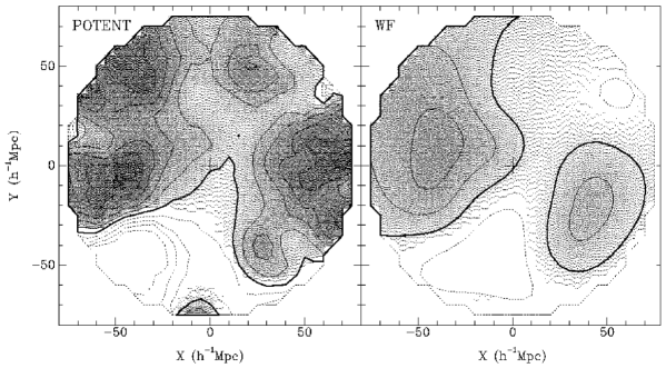
Figure 1: The density fields in the Supergalactic plane, recovered by POTENT (left) and WF (right) from the Mark III catalog of peculiar velocities. The formal Gaussian smoothing scale is $12\,h^{-1}{\rm Mpc}$. The Local Group is at the center. The heavy contour marks the mean density, $\delta=0$, the dotted lines mark negative contours, and the contour spacing is $\Delta\delta=0.2$. Apparent are the Great Attractor on the left, the Perseus-Pisces attractor on the right, and the void in between.

The corresponding velocity fields, in the Supergalactic plane and projected onto it, are shown in the top-left panels of Figure 2 and Figure 3. Two other panels in these figures show the divergent and tidal components. The divergent fields are dominated by the two characteristic infall patterns into the two attractors, GA and PP, and the outflows from the voids in between. A bulk flow, if it exists, does not seem to be a dominant feature of the divergent component. The tidal field, on the other hand, is clearly dominated by a coherent bulk velocity.

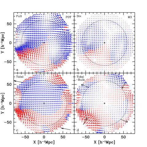
Figure 2: Decomposition of the POTENT velocity field in the Supergalactic plane, with respect to the sphere of $60\,h^{-1}{\rm Mpc}$ about the Local Group (center). The Velocities are measured in $\!\,h^{-1}{\rm Mpc}$ ($1\,h^{-1}{\rm Mpc}=100\,{\rm km}\,{\rm s}^{-1}$). (a) The full velocity field. (b) The divergent component due to the mass fluctuations within the sphere (shown in Figure 1. (c) The tidal component due to the mass distribution outside the sphere. (d) The residual after subtracting the bulk velocity from the tidal component, including quadrupole and higher moments. The black long arrows in the bottom panels show the projected directions of the bulk velocity and two of the shear eigenvectors respectively. (The red and blue in the upper panels correspond to positive and negative $\kern-0.22495pt\hbox{$\nabla$}\kern-7.50002pt\kern 0.45003pt\hbox{$\nabla$}\kern-7.50002pt\kern-0.22495pt\raise 0.38974pt\hbox{$\nabla$}\cdot\kern-0.22495pt\hbox{$v$}\kern-4.68541pt\kern 0.45003pt\hbox{$v$}\kern-4.68541pt\kern-0.22495pt\raise 0.38974pt\hbox{$v$}$ respectively. In the bottom-left panel they distinguish between velocities according to whether the angle they form with the direction of the bulk velocity (long arrows) is larger or smaller than $30^{\circ}$. In the bottom-right panel the colors refer to the direction of the eigenvector with the largest eigenvalue.)

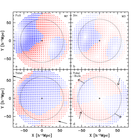
Figure 3: Same as Figure 2 but for the WF reconstruction.

4 TIDAL FIELD: BULK VELOCITY AND SHEAR

To analyze the tidal field in more detail, it is further decomposed into several components by fitting a linear model of the sort

$$v_{\alpha}(\kern-0.24994pt\hbox{$r$}\kern-4.78937pt\kern 0.50003pt\hbox{$r$}\kern-4.78937pt\kern-0.24994pt\raise 0.43304pt\hbox{$r$})=B_{\alpha}+(\tilde{H}\,\delta_{\alpha\beta}+\Sigma_{\alpha\beta})r_{\beta}\ .$$ (6)

Here, the indices $\alpha$ and $\beta$ refer to the 3 Cartesian coordinates, $B_{\alpha}$ is the bulk velocity, $\tilde{H}\delta_{\alpha\beta}$ accounts for a possible local isotropic perturbation about the Hubble expansion ($\delta_{\alpha\beta}$ is the identity matrix), and $\Sigma_{\alpha\beta}$ is the traceless shear tensor. In the terminology of potential theory, the bulk and shear terms are the dipole and quadrupole respectively. The expansion does not contain an antisymmetric part because the flow is assumed to be irrotational. The fit is done by an unweighted volume average over the grid points inside the reference volume. In the case of the tidal field the isotropic term, $\tilde{H}\delta_{\alpha\beta}$, vanishes by construction, because it corresponds to the divergent component of the flow.

The traceless shear tensor is then diagonalized, and we denote its eigenvalues in decreasing order $\lambda_{1}>\lambda_{2}>\lambda_{3}$, where $\lambda_{1}+\lambda_{2}+\lambda_{3}=0$. The eigenvalues $\lambda_{1}$ and $\lambda_{3}$ correspond to the dilational and compressional modes respectively.

The fourth panels of Figure 2 and Figure 3 show the result of subtracting the bulk velocity from the tidal field. This field is dominated by a clear quadrupole pattern, for which the Supergalactic plane is close to a principal plane. The eigenvector of the largest eigenvalue lies along the line from bottom-right to top-left.

4.1 Bulk Velocity of the Tidal Field

Figure 4 shows the amplitude of the bulk velocity in the CMB frame, averaged in spheres of radius $R$ about the Local Group. Shown are the total bulk velocity and its two components, divergent and tidal. The divergent contribution is significant at small radii, indicating that local density structures like GA and PP are responsible for up to one half of the Local-Group velocity. The divergent bulk velocity tends to zero towards $R=60\,h^{-1}{\rm Mpc}$. Note that this is not guaranteed a priori; a nonzero bulk flow can in principle be associated with local perturbations (e.g., in the case of a dominant attractor near the edge of the volume). The vanishing divergent bulk velocity reflects the general mirror symmetry between GA and PP.

The tidal bulk velocity from POTENT is $366\pm 125\,{\rm km}\,{\rm s}^{-1}$ in the direction $(L,B)=(167^{\circ},\,-10^{\circ})$, and from WF it is $309\pm 125\,{\rm km}\,{\rm s}^{-1}$ in the direction $(L,B)=(165^{\circ},\,-15^{\circ})$. The two methods yield very similar directions that differ by only $8^{\circ}$. The amplitudes are consistent with each other; they differ in the direction expected due to the differences between the methods as explained in § 2. The two tidal bulk velocities form an angle of $\sim 34^{\circ}$ and $\sim 26^{\circ}$ respectively with the Local Group motion in the CMB frame, implying, again, that about half of this Local-Group velocity, of $627\pm 22\,{\rm km}\,{\rm s}^{-1}$ (Lineweaver et al. 1996), is induced by density structures on scales beyond $60\,h^{-1}{\rm Mpc}$.

Figure 4: The amplitude of bulk velocity in the CMB frame in spheres of radius $R$ about the Local Group. It is derived by equal-volume vector averaging of the POTENT (left) and WF (right) velocity fields. Shown are the total bulk velocity and its two components, divergent and tidal. The error bars mark random errors, and the arrows mark crude estimates of systematic errors (POTENT only).

Figure 5 shows the direction of the bulk velocity as a function of sphere radius, for the full velocity field, and for its two components. The WF reconstruction reveals a very robust direction for the bulk velocity, as expected, while the directions in the POTENT case fluctuate a bit more due to the random errors at radii larger than $40\,h^{-1}{\rm Mpc}$.

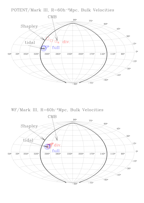
Figure 5: The directions of the full bulk velocity and its divergent and tidal components, in Galactic coordinates. The bulk velocities are derived inside spheres of radii $20,30,...60\,h^{-1}{\rm Mpc}$, and the circle size is proportional to the sphere radius.

4.2 Shear Tensor of the Tidal Field

As seen in Figure 2 and Figure 3, the residual tidal field after the bulk velocity is subtracted out is dominated by a quadrupole whose dilational eigenvector is roughly aligned with the direction to the Shapley Concentration.

The one-dimensional rms residual about the linear fit, ($\sigma_{\rm v}$), which is almost the same in the three directions, is $\sigma_{\rm v}\simeq 145\,{\rm km}\,{\rm s}^{-1}$ for POTENT and $\simeq 28\,{\rm km}\,{\rm s}^{-1}$ for WF. The eigenvalues for the POTENT field are $0.037\pm 0.029$, $0.008\pm 0.032$, and $-0.045\pm 0.027$. For the WF field they are quite consistent: $0.036\pm 0.007$, $-0.003\pm 0.009$, and $-0.033\pm 0.007$.

Figure 6 shows the directions of the bulk velocity and the three shear eigenvectors of the tidal field. The uncertainties about these directions are evaluated by applying the tidal field decomposition to 10 random mock catalogs (POTENT) and CRs (WF). The resultant spread in directions is shown in the figure.

Although the dilational eigenvectors as obtained from the two reconstruction methods are about $70^{\circ}$ apart, given the uncertainties they are both not that far from the direction of the tidal bulk velocity (deviations of $\sim 30^{\circ}$ for POTENT and $\sim 50^{\circ}$ for EF), and they are both in the crude general direction of the Shapley concentration. The corresponding compressional eigenvectors are only about $17^{\circ}$ from each other, while the middle eigenvectors are very uncertain and are quite far apart.

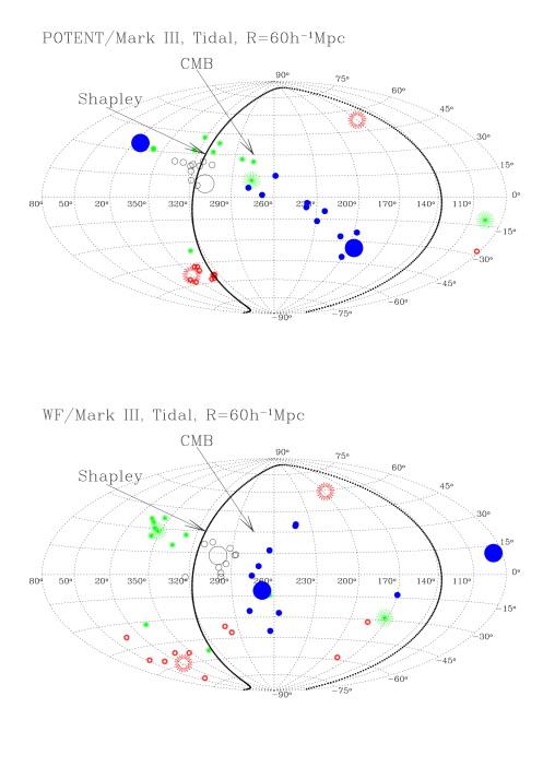
Figure 6: The directions of the tidal bulk velocity (open circles), and the three eigenvectors of the shear: the dilation (skeletals), the compression (starred), and the middle-eigenvalue vector (solid). The large symbols are for the real data, and the corresponding small symbols are for 10 random realizations generated by mock catalogs for the POTENT and by CRs for WF. Also shown are the anti-apex of the three eigenvectors.

4.3 Sensitivity of WF to the Prior Power Spectrum

We examine here the sensitivity of our WF tidal results to the assumed prior power-spectrum. The maximum-likelihood determination of the power-spectrum parameters (Zaroubi et al. 1997), for tilted, flat $\Lambda$CDM, COBE normalized with tensor fluctuations, put $1\sigma$ constraints on a degenerate combination of the parameters, roughly $\Omega h_{50}^{1.3}n^{3.4}=0.8\pm 0.12$ (where $h_{50}\equiv H_{0}/50\,{\rm km\,s^{-1}Mpc^{-1}}$).

Table 1: Sensitivity of the Tidal Bulk and Shear to the Prior Power Spectrum

$\Delta(\Omega h^{1.3}n^{3.4})$	$\Omega$	$h$	$n$	$B_{t}(\,{\rm km}\,{\rm s}^{-1})$	$(L,B)$	$\lambda_{1}$	$\lambda_{2}$	$\lambda_{3}$
0	1	0.75	0.81	309	$(164.5^{\circ},-15.0^{\circ})$	0.036	-0.033	-0.003
0	0.5	0.75	0.993	343	$(165.2^{\circ},-15.1^{\circ})$	0.048	-0.041	-0.007
0	1	0.60	0.882	322	$(164.7^{\circ},-15.2^{\circ})$	0.040	-0.036	-0.004
-0.12	0.855	0.75	0.81	315	$(165.3^{\circ},-14.9^{\circ})$	0.038	-0.034	-0.004
-0.12	1	0.75	0.7735	305	$(165.0^{\circ},-14.8^{\circ})$	0.034	-0.031	-0.003
-0.12	1	0.665	0.81	313	$(165.2^{\circ},-14.9^{\circ})$	0.037	-0.033	-0.004
+0.12	1	0.75	0.843	311	$(164.0^{\circ},-15.2^{\circ})$	0.037	-0.034	-0.003

In Table 1 we present the results extracted from several WF reconstructions using different values for $\Omega$, $h_{50}$ and $n$ that obey the maximum-likelihood constraint, as well as various combinations of these parameters that lie on the $1\sigma$ likelihood contour. The table displays the resultant tidal-field quantities of bulk velocity and shear. The variations in the bulk velocity are less than $10\%$ in magnitude and $1^{\circ}$ in direction. The variations in the eigenvalues of the shear tensor are typically $10-30\%$. The WF results are thus quite robust.

4.4 Preliminary Results from SFI

The method described in this paper is being applied to other data sets and compared to complementary information from redshift surveys (in preparation). To have a feeling for the robustness of our obtained tidal field, we briefly describe here preliminary results from the SFI catalog of peculiar velocities (Haynes et al. 1999a,b). This catalog contains Tully-Fisher distances for $\sim 1300$ Sc galaxies. Its spatial extent is similar to the Mark III sample, but the sampling is sparser and more uniform throughout the volume. Malmquist bias has been corrected in SFI as explained in Freudling et al. (1999).

Figure 7 shows the decomposition of the POTENT velocity field from the SFI data, similar to Figure 2 for Mark III. Note the similarity between the recovered tidal fields from the two data sets. The best-fit tidal bulk velocity of SFI is $255\,{\rm km}\,{\rm s}^{-1}$ towards $(L,B)=(165,\,-17)$, which is fully consistent with that of Mark III. The directions of the shear eigenvectors are also very similar for the two data sets, with SFI eigenvalues $(0.068,\,0.008,\,-0.076)$, repeating the pattern of two eigenvalues with comparable absolute values. Despite the large uncertainties, the tidal field is surprisingly robust.

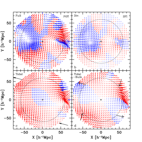
Figure 7: Same as Figure 2, but for the SFI data.

5 THE SHAPELY ATTRACTOR

The components of the shear tensor provide an indication for the source of the tidal field, which we saw is responsible for about one half of the Local Group velocity. Since the bulk velocity and the dilational eigenvector point in the same general direction, it may be useful to fit the tidal field with a toy model of a single attractor — a point-mass or a sphere of mass excess $\delta M$ centered at a distance $D$ from the Local Group. Within that model the distance is estimated by $D\sim 2B/\lambda_{1}$. Given the values obtained above from the Mark III data we estimate

$$D\sim(150-200)\,h^{-1}{\rm Mpc}\ .$$ (7)

In linear theory this fluctuation generates a velocity field

$$v(\kern-0.24994pt\hbox{$r$}\kern-4.78937pt\kern 0.50003pt\hbox{$r$}\kern-4.78937pt\kern-0.24994pt\raise 0.43304pt\hbox{$r$})={2f(\Omega)\over 3\Omega}{G\,\delta M\over H_{0}D^{2}}\ .$$ (8)

Substituting the estimated value of $D$, we obtain

$$\delta M\sim(2-5)\times 10^{17}M_{\odot}h^{-1}\Omega^{0.4}.$$ (9)

This single attractor model closely coincides with the Shapley Concentration of rich galaxy clusters. Reisenegger et al. (2000), who studied the dynamics of the Shapley Concentration, obtained using a spherical infall model an upper limit of $M<1.3\times 10^{16}M_{\odot}h^{-1}$ (for an Einstein-de Sitter universe) and $M<8.5\times 10^{15}M_{\odot}h^{-1}$ (for an empty universe), consistent with the predictions of our toy model. They located the Shapley supercluster at a redshift $z\approx 0.048$, close to our estimate of $D$. The direction of the Shapley Concentration lies close to the directions of the bulk velocity and the dilational eigenmode of the tidal field, and almost in between. These all point to the important role of the Shapley Concentration in inducing the tidal field within the local sphere of $60\,h^{-1}{\rm Mpc}$.

However, this indication should not be overinterpreted. The single attractor model is clearly an oversimplification which provides only a limited fit to the data. This is manifested by the eigenvalue ratio of $\lambda_{3}/\lambda_{1}\simeq-1$ for the real tidal shear tensor, compared to the predicted value of $-0.5$ of the single-attractor model. Shapley is likely to be an important tidal source, but it is certainly not the only relevant external perturbation.

A better fit to the tidal field is provided by a slightly more complicated toy model which includes one point-mass attractor and two negative point masses representing voids of density below the cosmological average. We fix the attractor position roughly at the Shapely Concentration, at a distance of $150\,h^{-1}{\rm Mpc}$ in the Supergalactic direction $(L,B)=(142^{\circ},0^{\circ})$, and allow the associated mass to be a free parameter. Two voids are allowed, with free masses and free positions, limited to lie outside the volume boundary of $60\,h^{-1}{\rm Mpc}$ and inside $100\,h^{-1}{\rm Mpc}$. This toy model has 9 free independent parameters, while there are 8 constraints imposed by the tidal bulk velocity and shear tensor. A perfect solution is not guaranteed even when the number of parameters matches the number of constraints because the system of equations is nonlinear, and because we limit the search volume to $100\,h^{-1}{\rm Mpc}$. We determine the errors for each component using mock catalogs based on simulations, and determine the best-fit parameters by minimizing the sum of residuals over the 8 components:

$$\sum_{\alpha}{(B^{\rm model}_{\alpha}-B^{\rm obs}_{\alpha})^{2}\over\sigma_{B_{\alpha}}^{2}}+\sum_{\alpha,\beta}{(\Sigma^{\rm model}_{\alpha\beta}-\Sigma^{\rm obs}_{\alpha\beta})^{2}\over\sigma_{\Sigma_{\alpha\beta}}^{2}}\ .$$ (10)

The model bulk velocity is the sum of the contributions of each of the three point masses, of the sort $2f(\Omega)G/(3\Omega H_{0})\,\delta M\,r_{\alpha}/r^{3}$, and the model shear is similarly a sum of the three contributions of the sort $2f(\Omega)G/(3\Omega H_{0}^{2})\,\delta M\,(3\hat{r}_{\alpha}\hat{r}_{\beta}-\delta_{\alpha\beta})/r^{3}$.

The best toy model we found has an attractor mass of $1.6\times 10^{17}M_{\odot}h^{-1}$, and effective masses of $-0.5\times 10^{17}M_{\odot}h^{-1}$ associated with each of the two voids, located at $(D,L,B)=(88\,h^{-1}{\rm Mpc},54^{\circ},0^{\circ})$ and $(100\,h^{-1}{\rm Mpc},324^{\circ},11^{\circ})$ respectively. Note how close these structures are to the Supergalactic Plane. Figure 8 shows the positions of these three elements of the toy model on top of the map of the density and velocity fields in the Supergalactic Plane as derived from the PSCz redshift survey of IRAS galaxies (Schmoldt et al.  1999). One void lies roughly along the principal mode of dilation, namely along the line connecting the Local Group with Shapely but to the opposite direction, behind the Perseus Pisces (PP) supercluster. The other void lies in an orthogonal direction, behind the nearby Ursa Major (UM) cluster. The tidal bulk velocity induced by this toy model is only about $20^{\circ}$ away from the real bulk velocity by POTENT from Mark III. The shear eigenvalues of the toy model are $(0.029,0.012,-0.041)$, compared to the real eigenvalues $(0.037,0.008,-0.045)$, and they point in directions that are less than $15^{\circ}$ away from the real directions. This toy model is thus quite successful.

Note in Figure 8 that the dynamical voids indicated by the tidal field indeed lie in the vicinity of two out of a few extended voids as seen in the PSCz map. Another void is apparent along the line connecting the Local Group to the UM void but in the opposite direction, termed the Sculptor void. A fit of somewhat lower quality but still with the right main features is obtained by a toy model in which the PP void is replaced by a void in the vicinity of Sculptor.

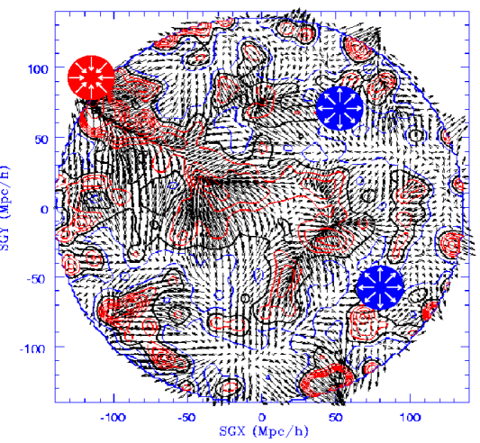
Figure 8: A 3-mass toy model on top of the PSCz galaxy distribution in the Supergalactic Plane. Marked are the positions of the attractor and two voids, in the toy model that best fits the tidal field as derived by POTENT from Mark III. Shown at the background are the density and velocity fields from the PSCz redshift survey of IRAS galaxies. The Local Group is at the center. The structures towards the top-left are the Great Attractor in the foreground and the Shapely Concentration in the background. The structure to the opposite direction is Perseus Pisces. The Come Supercluster is at a distance of $\sim 70-80\,h^{-1}{\rm Mpc}$ towards the top. Ursa Major is a nearby cluster towards top-right.

6 CONCLUSION

The main purpose of this paper was to present an algorithm for the decomposition of the large-scale tidal velocity field. The algorithm is based on solving the linear Poisson equation given the reconstructed density field inside a certain volume, while assuming that the fluctuations vanish outside the volume. The tidal field is then obtained by subtracting this particular solution from the full reconstructed velocity field.

This algorithm has been applied to the velocity and density fields recovered from the Mark III peculiar-velocity data by the complementary POTENT and WF methods. The tidal field was calculated with respect to the sphere of radius $60\,h^{-1}{\rm Mpc}$ about the Local Group.

The tidal field is characterized by a bulk velocity and a shear tensor. We found that about half the amplitude of the CMB dipole is due to mass-density fluctuations outside the reference sphere. The dilational eigenvector (with the largest eigenvalue) of the shear tensor is roughly aligned with the bulk velocity, which indicates the important dynamical role of an attractor of mass $(2-5)\times 10^{17}M_{\odot}h^{-1}\Omega^{0.4}$ at a distance of $150-200\,h^{-1}{\rm Mpc}$, behind the Great Attractor, roughly coinciding with the Shapley Concentration. However, the tidal field must also involve additional structures. The addition of two voids in the Supergalactic Plane improves the fit: one void behind the Ursa Major cluster, and the other either behind the Perseus-Pisces supercluster or the Sculptor void in an orthogonal direction. These roughly coincide with voids in the PSCz redshift survey.

Our conclusions are strengthened by the agreement between the results obtained using the two complementary reconstruction methods, which treat the random errors in very different ways. The two estimators are likely to bracket the actual amplitude of the tidal field.

The obtained tidal field from the SFI data is consistent with that obtained from the Mark III data, which is quite surprising in view of the expected large errors. Consistency with other data and its implications are now under investigation.

The tidal field we find have implications for the issue of convergence of the bulk velocity as measured from different velocity surveys on different scales (a summary in Dekel 2000), and for the question of the effective depth for the recovery of the CMB dipole motion of the Local Group. The latter is crucial for evaluating the cosmological density parameter from the CMB dipole versus the dipole from a redshift survey (e.g., Lahav, Kaiser and Hoffman 1990; Juszkiewicz, Vittorio and Wyse 1990).

- (1)
- (2) Aaronson, M., Huchra, J., Mould, J. R., Tully, R. B., Fisher, J. R., van Woerden, H., Goss, W. M., Chamaraux, P., Mebold, U., Siegman, B., Berriman, G., and Persson, S. E, 1982, ApJS, 50, 241
- (3) Bertscinger, E. & Dekel,A., 1989. ApJ Lett., 336, L5
- (4) Courteau, S., Faber, S. M., Dressler, A., & Willick, J. A. 1993 ApJ, 412, L51
- (5) Dekel, A. 1999, in Formation of Structure in the Universe, eds. A. Dekel & J.P. Ostriker (Cambridge University Press) p. 250
- (6) Dekel, A. 2000, in Cosmic Flows: Towards an Understanding of Large-Scale Structure, eds. S. Courteau, M.A. Strauss, & J.A. Willick (ASP Conf. Series), in press (astro-ph/9911501)
- (7) Dekel, A., Bertschinger, E., & Faber, S.M. 1990, ApJ, 364, 349
- (8) Dekel, A., Eldar, A., Kolatt, T., Yahil, A., Willick, J. A., Faber, S. M., Courteau, S., & Burstein, D. 1999, ApJ, 522, 1
- (9) Dressler, A., Lynden-Bell, D., Burstein, D., Davies, R. L., Faber, S. M., Terlevich, R. J., Wegner, G. 1987, ApJ, 313, 42
- (10) Eldar, A., Dekel, A., & Willick, J. A. 1999, in preparation
- (11) Freudling, W., Zehavi, I., daCosta, L.N., Dekel, A., Eldar, A., Giovanelli, R., Haynes, M.P., Salzer, J.J., Wagner, G., & Zaroubi, S. 1999, ApJ, 523, 1
- (12) Górski, K.M. 1988, ApJ, 332, L7
- (13) Han, M.-S., & Mould, J. R. 1992, ApJ, 396, 453
- (14) Haynes, M. P., Giovanelli, R., Salzer, J. J., Wegner, G., Freudling, W., da Costa, L. N., Herter, T., & Vogt, N. P. 1999a, AJ, 117, 1668
- (15) Haynes, M. P., Giovanelli, R., Chamaraux, P., da Costa, L. N., Freudling, W., Salzer, J. J., & Wegner, G. 1999b, AJ, 117, 2039
- (16) Juszkiewicz,R., Vittorio, N., & Wyse, R.F.G., ApJ, 349, 408
- (17) Hoffman, Y., & Ribak, E. 1991, ApJ, 380, L5
- (18) Kolatt, T., Dekel, A., Ganon, G., & Willick, J. A. 1996, ApJ, 458, 419
- (19) Lahav, O., Kaiser, N. and Hoffman, Y., 1990, ApJ, 352, 448
- (20) Lilje, P. B., Yahil, A., & Jones, B. J. T. 1986, ApJ, 307, 91
- (21) Lineweaver, C. H, Tenorio, L., Smoot, G. F., Keegstra, P., Banday, A. J., & Lubin, P. 1996, ApJ, 470, 38
- (22) Lynden-Bell, D., Faber, S. M., Burstein, D., Davies, R. L., Dressler, A., Terlevich, R. J., & Wegner, G. 1988, ApJ, 326, 19
- (23) Mathewson, D. S., Ford, V. L, & Buchhorn, M. 1992, ApJS, 81, 413
- (24) Nusser, A., Dekel, A., Bertschinger, E., & Blumenthal, G. R. 1991, ApJ, 379, 6
- (25) Peebles, P.J.E., ‘’The Large-Scale Structure of the Universe”, 1980, Princeton University Press (Princeton, New Jersey)
- (26) Reisenegger, A., Quinana, H., Carrasco, E.R., & Maze, J., 2000, preprint (astro-ph/0007211)
- (27) Schmoldt, I.M., Saar, V., Saha, P., Branchini, E., Efstathiou, G.P., Frenk, C. S., Keeble, O., Maddox, S., McMahon, R., Oliver, S., Rowan-Robinson, M., Saunders, W., Sutherland, W.J., Tadros, H., & White, S.D.M., 1999, AJ, 118, 1146
- (28) Willick, J. 1990, ApJ, 351, L5
- (29) Willick. J.A. 1999, in Formation of Structure in the Universe, eds. A. Dekel & J.P. Ostriker (Cambridge University Press) p. 213
- (30) Willick, J. A., Courteau, S., Faber, S. M., Burstein, D., & Dekel, A. 1995, ApJ, 446, 1 (Mark III paper 1)
- (31) Willick, J. A., Courteau, S., Faber, S. M., Burstein, D., Dekel, A., & Kolatt, T. 1996, ApJ, 457, 460 (Mark III paper 2)
- (32) Willick, J. A., Courteau, S., Faber, S. M., Burstein, D., Dekel, A., & Strauss, M.A. 1997a, ApJS, 109, 333 (Mark III paper 3)
- (33) Yahil, A., Tammann, G. A., & Sandage, A. 1977, ApJ, 217, 90
- (34) Zaroubi, S., Hoffman, Y., Fisher, K. B., & Lahav, O. 1995, ApJ, 449, 446
- (35) Zaroubi, S., Zehavi, I., Dekel, A., Hoffman, Y., & Kolatt, T. 1997, ApJ, 486, 21
- (36) Zaroubi, S., Hoffman, Y., & Dekel, A., 1999, ApJ, 520, 413
- (37)