Study by MOA of extra-solar planets in gravitational microlensing events of high magnification

Abstract

A search for extra-solar planets was carried out in three gravitational microlensing events of high magnification, MACHO 98–BLG–35, MACHO 99–LMC–2, and OGLE 00–BUL–12. Photometry was derived from observational images by the MOA and OGLE groups using an image subtraction technique. For MACHO 98–BLG–35, additional photometry derived from the MPS and PLANET groups was included. Planetary modeling of the three events was carried out in a super-cluster computing environment. The estimated probability for explaining the data on MACHO 98–BLG–35 without a planet is $<1$%. The best planetary model has a planet of mass $\sim(0.4-1.5)\times M_{\rm Earth}$ at a projected radius of either $\sim 1.5$ or $\sim 2.3$ AU. We show how multi-planet models can be applied to the data. We calculated exclusion regions for the three events and found that Jupiter-mass planets can be excluded with projected radii from as wide as about 30 AU to as close as around 0.5 AU for MACHO 98–BLG–35 and OGLE 00-BUL-12. For MACHO 99–LMC–2, the exclusion region extends out to around 10 AU and constitutes the first limit placed on a planetary companion to an extragalactic star. We derive a particularly high peak magnification of $\sim 160$ for OGLE 00–BUL–12. We discuss the detectability of planets with masses as low as Mercury in this and similar events.

1 Introduction

A remarkable diversity of planetary systems has been uncovered in recent years through studies of extra-solar planets (Mayor & Queloz 1995, Marcy & Butler 1998, Perryman 2000). Many further studies will be required to obtain a full understanding of this diversity of planetary systems and their formation processes. In this paper we report a study of extra-solar planetary systems using a gravitational microlensing technique.

Table 1: Observational datasets used here. The red and blue passband filters used by MOA were 630–1000 nm and 400–630 nm respectively (Yanagisawa et al. 2000). We used difference imaging analysis on those datasets comprised of raw images. The MPS and PLANET datasets are based on DoPHOT analyses previously carried out by the respective groups.

Event	Telescope	Location	Passband	Number of	Data Source
				Data Points
MACHO 98–BLG–35	MOA 0.6-m	NZ	red	162	Images from MOA-camI
	MPS 1.9-m	Australia	R	128	Rhie et al. (2000)
	PLANET 1-m	S. Africa	I	3	PLANET website
	PLANET 1-m	S. Africa	V	5	PLANET website
	PLANET 1-m	Australia	I	20	PLANET website
	PLANET 1-m	chile	I	18	PLANET website
	PLANET 1-m	chile	V	8	PLANET website
MACHO 99-LMC-2	MOA 0.6-m	NZ	red	341	Images from MOA-camII
	MOA 0.6-m	NZ	blue	346	Images from MOA-camII
	OGLE 1.3-m	chile	I	219	Images provided by OGLE
OGLE 00-BUL-12	OGLE 1.3-m	chile	I	300	Images provided by OGLE

Mao and Paczynski (1991) pointed out that extra-solar planets could be detected using gravitational microlensing, because the characteristic scale in gravitational microlensing happens to coincide quite closely with the characteristic size of the solar system. The characteristic scale of gravitational microlensing is the radius of the Einstein ring, $R_{\rm E}$, which is

$$R_{\rm E}=\sqrt{\frac{4GM_{\rm L}}{c^{2}}}\times\sqrt{\frac{D_{\rm OL}D_{\rm LS}}{D_{\rm OS}}}.$$ (1)

Here $M_{L}$ denotes the mass of the lens, and $D_{\rm OL}$, $D_{\rm LS}$ and $D_{\rm OS}$ the distances from the observer to lens, lens to source and observer to source respectively. For microlensing events that occur in the galactic bulge, $M_{\rm L}$ is typically $\sim 0.3M_{\odot}$, and $D_{\rm{OL}}$, $D_{\rm{LS}}$ and $D_{\rm{OS}}$ are typically about 6 kpc, 2 kpc and 8 kpc respectively. These values imply $R_{\rm E}\sim$ 1.9 AU. Consequently, if other planetary systems have the same characteristic size as ours, planets orbiting a lens star may perturb the lensing, because light from the source star may pass close to one or more of the planets at some time during a microlensing event. Gould & Loeb (1992) and Bolatto & Falco (1994) showed that Jupiter-like planets could be detected with about 20% efficiency in typical microlensing events if they are monitored at about hourly intervals with a photometric precision of a few per cent throughout each event. The PLANET collaboration has used this technique to set an upper limit on the abundance of Jupiter-like planets of order 30% (Albrow et al. 2001). This result is consistent with results obtained independently by radial velocity and transit measurements (Marcy & Butler 1998, Charbonneau et al. 2000, Henry et al. 2000, Jha et al. 2000). Bennett & Rhie (2000) emphasized the detectability of terrestrial planets by microlensing where they showed that Earth-mass planets could be detected with about 5% efficiency in typical events if they are monitored hourly at a photometric precision of better than 1%.

A modification of the gravitational microlensing plant search strategy was pointed out by Griest & Safizadeh (1998) in which planets, including those less massive than Jupiter, could be detected with high efficiency in microlensing events of high magnification. This occurs when the distance of closest approach of the lens star to the line-of-sight to the source star, $u_{\rm min}$, is much smaller than the Einstein radius, i.e. when $u_{\rm min}\ll 1$ where $u_{\rm min}$ is expressed in units of $R_{\rm E}$. In these events a circular, or near-circular, image generally forms around the lens with radius $R_{\rm E}$ at the time of maximum amplification, and the maximum amplification $A_{\rm max}\approx 1/u_{\rm min}\gg 1$. If a planet is orbiting the lens star at a projected radius of about a few AU at the time of an event, it will perturb the image, although the perturbation will be small because most of the image will lie far from the planet and remain unperturbed. For planets with masses as low as that of Earth, simulations show (see §5 below) that the perturbation may nevertheless be detectable with appropriate observations. The aim of the present study was to exploit this sensitivity.

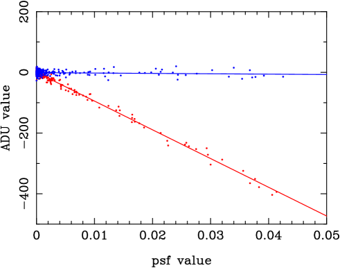
Figure 1: Fits of empirical PSF profiles to profiles on a subtracted image. The falling fit is for the profile on the first subtracted image at the position of MACHO 98–BLG–35. The horizontal fit is for one of the vast majority of stars that do not change and are well subtracted. The slope of any fit provides the $\Delta F$ measurement, and the standard deviation from the fit provides a measurement of the quality of the image subtraction.

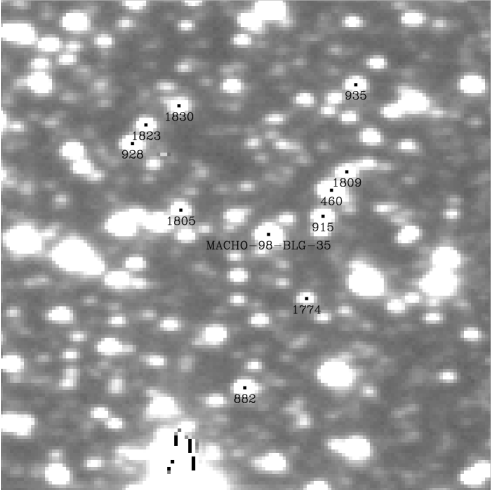
Figure 2: Sub-region of the reference image used in the difference imaging analysis of the MOA dataset on MACHO 98–BLG–35. This image was constructed by combining four of the best seeing images which occurred during the times of peak brightness of the event. Also shown are the position of ten objects selected as check stars. The camera MOA-cam1, with a pixel size on the sky of 0.65″, was used for these exposures.

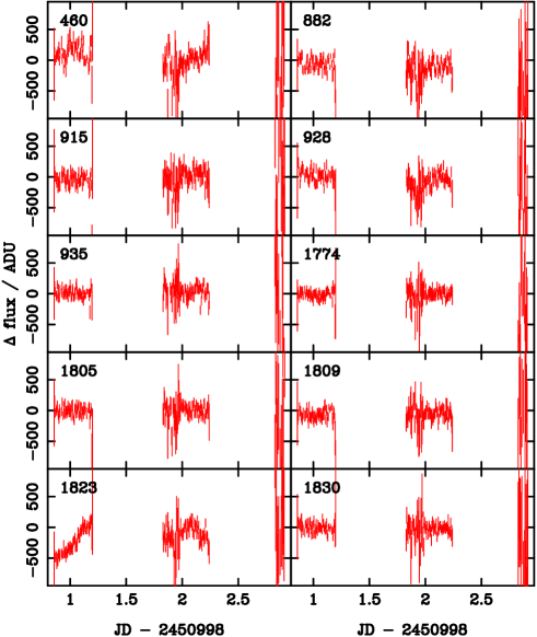
Figure 3: Light curves of ten check stars for MACHO 98–BLG–35 on the peak night and on the following two nights. Stars 460, 928 and 1823 appear to have varied on both nights 1 and 2. The presence of thin cloud during the second quarter of the second night and of thick cloud on the third night is apparent.

The first analysis of a high amplification event in terms of planets was reported by Rhie et al. (2000). These authors reported a low-mass planetary signal (few Earth masses to few Uranus masses) at a marginal level of confidence for the event MACHO 98–BLG–35, and excluded Jovian planets over an extensive region surrounding the lens star. They also pointed out that further such results in additional events would provide statistically significant constraints on the abundance of Earth-mass planets, but that more accurate planetary parameters can be obtained in events in which a ”planetary caustic” is crossed or approached, which generally occurs at lower magnifications.

In this paper we report a re-analysis of MACHO 98–BLG–35, where the data in Rhie et al (2000) obtained by MOA have been analysed using an improved technique based on image subtraction and the inclusion of additional data. We also report analyses of two more events of high magnification, MACHO 99–LMC–2 and OGLE 00–BUL–12. We note that the event MACHO 99–LMC–2 coincides with the event OGLE 99–LMC–1 that was found independently by the OGLE group.

2 Observational Datasets

Data from the MOA (Abe et al. 1997), OGLE (Udalski et al. 1997), MPS (Bennett et al. 1999) and PLANET (Albrow et al. 2001) microlensing groups were used in the present analysis. The datasets are summarized in Table 1. Wherever possible, we attempted to obtain actual images and analyse these using an image subtraction procedure to achieve optimum photometric precision in the dense stellar fields in which microlensing is observed. The reduced datasets so obtained are posted at the MOA website.

Observations of MACHO 98–BLG–35 and MACHO 99–LMC–2 by MOA were made with the cameras MOA-cam1 and MOA-cam2 respectively (Yanagisawa et al. 2000). We note here that MOA-cam2 was operating in a slightly non-linear mode during 1999, and that the MOA data on MACHO 99-LMC-2 were corrected for this on a pixel-by-pixel basis using linearly calibrated stars from observations made in 2000.

Datasets on MACHO 98–BLG–35 by the MPS and PLANET groups were included in the present analysis. These datasets were reduced by these groups using the DoPHOT procedure of Schechter et al. (1993) and posted at their websites. In the case of the MPS dataset, it is the same dataset that was used previously by Rhie et al. (2000). In the case of the PLANET dataset, the data used here were obtained by extracting the unpublished, graphical data at the PLANET website, and allowing for a time offset of 0.007 day (A. Gould, private communication, 2000). The accuracy of the graphical extraction was much better than the error bars on the data. This may be seen by comparing the PLANET data shown in Fig. 10 of the present paper (see below) with Fig. 19 of their subsequent publication (Gaudi et al 2002). The need for the time offset, which was presumably caused by a heliocentric correction and/or simple clock errors of a few minutes, became clearly evident from comparisons of the raw PLANET and raw MPS/MOA datasets for the event

3 Image Subtraction Analysis

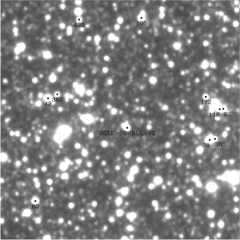
Figure 4: Sub-region of the reference image used in the difference imaging analysis of the OGLE datasets on OGLE 00-BUL-12 together with the positions of ten objects selected as check stars. The event itself is strongly blended on the image. Subsequently, a number of blended objects were selected as check stars. The plate scale here is 0.42″per pixel.

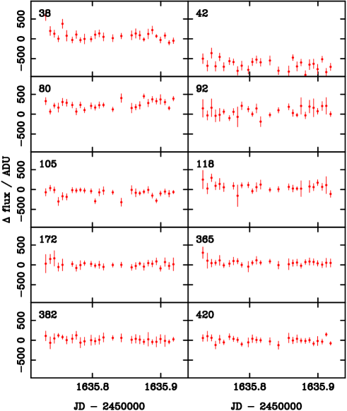
Figure 5: Light curves of ten check stars for OGLE 00-BUL-12 on the peak night. Stars 38 and 42 appear to have varied.

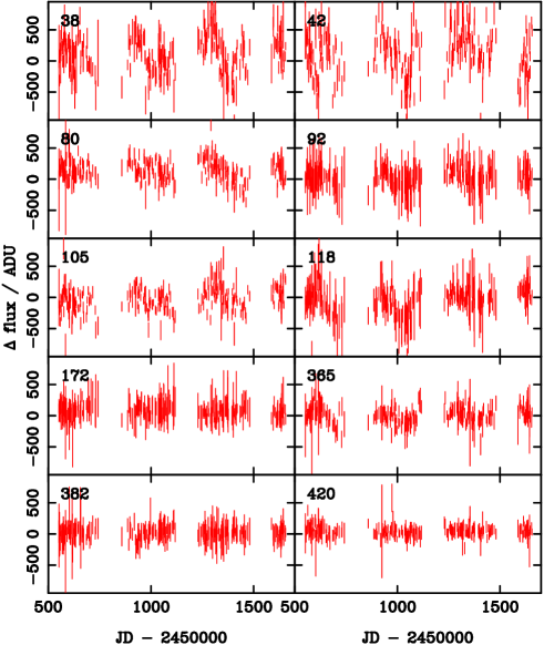
Figure 6: Light curves of the same stars as in Fig. 4 from 1997 to 2000. The stars 38 and 42 are confirmed as being variable on a time scale of one day.

The observations listed in Table 1 by the MOA and OGLE groups were reduced by an image subtraction procedure. Data from each telescope in each passband were treated as separate datasets. For each dataset, the flatfielded images were first geometrically aligned to an astrometric reference chosen from amongst the best seeing images. A reference image for the image subtraction process was then formed by stacking the very best seeing and signal-to-noise images. The convolution kernel which relates the seeing on the reference image to that for a particular image was then determined using our own implementation of the technique of Alard & Lupton (1998) for modeling the kernel along with the modification of Alard (1999) which models the spatial variations of the kernel across the CCD field of view.

Photometry on the subsequent dataset of subtracted images was carried out by first constructing an empirical point-spread-function (PSF) on the reference image using 5–6 bright, isolated stars near the event. A PSF for a particular image was then formed by convolving the reference PSF with the appropriate kernel. This PSF was fitted to the flux profile on the subtracted image at the position of a star to obtain a “delta-flux” measurement, $\Delta F$. The fit was done by re-aligning the centroid of the empirical PSF to that of the $\Delta F$ profile on the subtracted image, and performing a least squares fit to the pixel by pixel cross-plot of the two profiles. Typical fits are shown in Fig. 1.

Table 2: Parameters and statistics of the best single lens fits to the data obtained by the MOA and OGLE groups on the three events studied here and reduced by image subtraction. The uncertainties given correspond to $\Delta\chi^{2}=6.2$.

Event	$t_{\rm max}$	$t_{\rm E}$	$u_{\rm min}$	$A_{\rm max}$	$\chi^{2}$/dof
	JD$-$2450000	days
MACHO 98–BLG–35	999.15	$27.7\pm^{\infty}_{19.2}$	$0.0103\pm^{0.0539}_{0.0103}$	$96\pm^{\infty}_{81}$	329.1/157
MACHO 99-LMC-2	1337.24	$61.3\pm^{11.4}_{9.9}$	$0.0249\pm^{0.0049}_{0.0041}$	$40.3\pm^{7.8}_{6.7}$	1171.2/897
OGLE 00-BUL-12	1635.87	$69.4\pm^{27.6}_{15.4}$	$0.0063\pm^{0.0019}_{0.0018}$	$159.4\pm^{65.2}_{36.2}$	720.4/295

The scatter in fits such as those shown in Fig. 1 provides an indicator of the quality of the image subtractions. We used the standard deviation from the best fit straight line as a measurement of the subtraction quality associated with a given $\Delta F$ measurement. In a good quality subtraction, the profile of an object on the subtracted image should match that of the PSF on the unsubtracted image, and thus have a low standard deviation. Uncertainties in the $\Delta F$ measurements for any object were determined empirically. The profile fitting technique was applied to the positions of all resolved stars in the field. The frame-to-frame statistical errors for any particular object were then determined from the scatter in the $\Delta F$ values for stars with similar profile standard deviations.

Stars close to the microlensing events were selected as checks. Fig. 2 shows stars with similar statistical profile errors as MACHO 98–BLG–35, and Fig. 3 shows their light curves. Figs. 4–6 show similar stars from the OGLE database on OGLE 00–BUL–12. It is evident from these that the systematic errors in the image subtraction reduction procedure are significantly less than the statistical errors, and that the statistical errors are realistic.

4 Single Lens Fitting

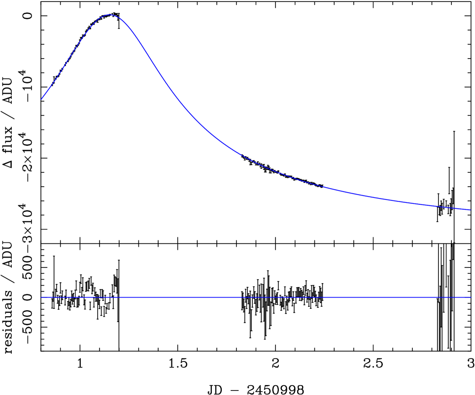
Figure 7: Light curve for MACHO 98–BLG–35 obtained by the MOA group in the red passband using subtraction photometry. The best single lens fit to the data is also shown. Thick cloud cover occurred on the third night, and thin cloud cover was present during the second quarter of the second night.

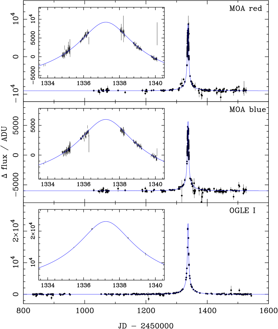
Figure 8: Light curves in the red, blue and I passbands for MACHO 99-LMC-2 on two time scales, and the best single lens fit to the data. The red and blue passband data are by MOA, and the I passband data are by OGLE. All the images were reduced by MOA using subtraction photometry as described in section 3.

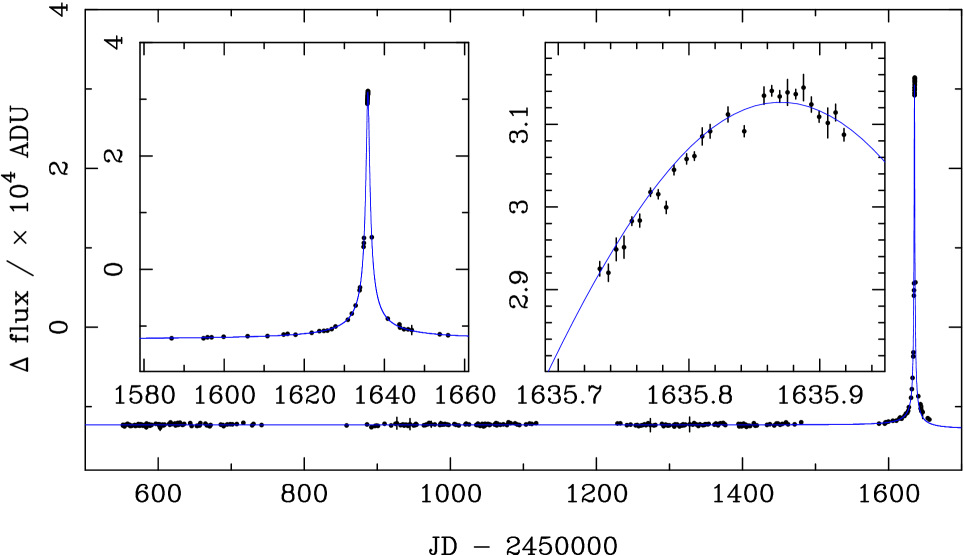
Figure 9: Light curve in I for OGLE 00-BUL-12 on three time scales, and the best single lens fit to the data. The images were supplied by the OGLE group and reduced by the MOA group using subtraction photometry.

For the datasets that were obtained by image subtraction the fluxes in any passband were fitted to the function

$$\Delta F(t)=F_{\rm b}A(u(t))-F_{\rm r}$$ (2)

where $F_{\rm b}$ denotes the baseline flux of the source star, and $F_{\rm r}$ is the source flux on the reference image used in the image subtraction process, which in general contains some lensed flux.

The well known amplification factor, $A(u)$, expressed in terms of the distance $u$ of the lens star from the line-of-sight to the source star expressed in units of $R_{\rm E}$, is given by (Paczynski 1986)

$$A(u)=\frac{u^{2}+2}{u\sqrt{u^{2}+4}},$$ (3)

where

$$u(t)=\sqrt{u_{\rm min}^{2}+{\left(\frac{t-t_{\rm max}}{t_{\rm E}}\right)}^{2}}.$$ (4)

Here $u_{\rm min}$ is the minimum value of $u$ during an event and $t_{\rm max}$ is the time of maximum amplification, i.e. the time when $u=u_{\rm min}$. The quantity $t_{\rm E}$ is the time scale that characterizes an event. It is equal to $R_{\rm E}/v_{\rm T}$ where $v_{\rm T}$ is the transverse velocity of the lens with respect to the line-of-sight to the source. In fitting a single lens curve to photometry taken in one or more passbands for a given event, there are therefore three microlensing parameters and two flux parameters for each passband.

The light curves for the three events are shown in Figs. 7–9 together with the best single lens fits to the data. For MACHO 98–BLG–35 only the data obtained by the MOA group have been included, since these were the only data to be reduced by image subtraction. The light curve for this event appears to exhibit substantial deviations from the single lens fit near its peak, but not at other times, suggestive of the presence of a planet (or planets) orbiting the lens star. Other possible causes of a deviation near the peak include the source star being a binary or having starspots. The binary interpretation seems unlikely (Rhie et al 2000). Also it would seem that starspots are unlikely to produce perturbations of the same strength as planetary deviations except in extreme situations (Rattenbury et al 2002, submitted to MRAS). For MACHO 99-LMC-2 no data were available to us at the peak, and in this case no apparent deviation from the single lens light curve is seen. For OGLE 00-BUL-12 there appears to be a possible deviation near the peak. The parameters and statistics of the single lens fits are displayed in Table 2.

We note that the maximum magnification determined for OGLE 00-BUL-12 by image subtraction, $A_{\rm max}=159$, is considerably higher than the value of 50 first reported by the OGLE Early Warning System. It should be noted that the first analysis was carried out using DoPHOT and that there is a significant degree of blending present in this event. This would underestimate the fitted value for the peak magnification. On the other hand, the light curve presented here is based on image subtraction photometry and should be unaffected by blending.

5 Planetary Modeling

We used the inverse ray shooting technique of Wambsganss (1997) to simulate lensing by planetary systems of arbitrary complexity, by firing photons from the telescope through the lens system to the plane of the source star. For every component of the lens system a deflection $4GM/bc^{2}$ was applied, where $b$ denotes impact parameter. Photons that hit the source star were retained; those that missed were discarded. In this way the finite size of the source star was allowed for, but the lens was treated in the thin-lens approximation. All the lens components were treated as if they were in a plane perpendicular to the ray direction. This treatment is expected to be sufficiently accurate because the dimensions of the lens system are much smaller than the distances between the lens and the observer, and the lens and the source.

The general procedure that was followed for planetary modeling was to calculate the $\chi^{2}$ values of the data for a broad range of planetary models to find the model with the smallest $\chi^{2}$. The light curve for any particular planetary model was calculated using the inverse ray shooting technique described above. Unless otherwise stated, the computations for all events corresponded to the following assumed values of the lens and source star parameters: $M_{L}=0.3M_{\odot}$, $D_{\rm OL}$=6 kpc, $D_{\rm LS}$=2 kpc and $R_{S}=R_{\odot}$. These values correspond to $D_{\rm OS}=8$ kpc and $R_{\rm E}$ = 1.9 AU. The coordinate system used for the computations is depicted in Fig. 10.

For the planetary modeling, the ratio of planet-to-lens mass $\epsilon$ was initially allowed to vary from $10^{-7}$ to $10^{-3}$ in 33 approximately equally logarithmically spaced steps for each event. Similarly, the projected coordinates of a planet $x_{\rm p}$ and $y_{\rm p}$ at the time of peak magnification were allowed to vary from $-2R_{\rm E}$ to $+2R_{\rm E}$ in 129 equally spaced steps. Thus a total of 549,153 planetary configurations was initially trialed for each event. The trialing was done on a super-cluster computer described by Rattenbury et al. (2002). For each trial, the $\chi^{2}$ was calculated over the time interval $-t_{\rm E}$ to $+t_{\rm E}$. This corresponds to the source star traversing the diameter of the Einstein ring. Maps of $\chi^{2}$ over the lens plane for the 33 planetary mass fractions were examined to determine approximate positions and masses of possible planets. Further minimization, described below, was subsequently carried out to determine the most likely planetary models.

5.1 MACHO 98–BLG–35

Planetary modeling of MACHO 98–BLG–35 was carried out using the combined dataset from MOA, MPS and PLANET. A typical $\chi^{2}$ map is shown in Fig. 11. This corresponds to an Earth-mass planet ($\epsilon=10^{-5}$). The minima on these maps indicate possible positions of planets at the time of the microlensing event. Maps for heavier (lighter) planets are similar, with the minima displaced further from (closer to) the Einstein ring. The Einstein ring is generally depicted clearly on these maps, either as a region where planets are strongly excluded, or where they may be present. The maps also depict a degeneracy that exists in the microlensing method, namely that planets at projected radii $a$ and $1/a$ (expressed in units of the Einstein radius) yield similar light curves, and hence are indistinguishable in this method (Griest & Safizadeh 1998).

The $\chi^{2}$ map shown in Fig. 11 for MACHO 98–BLG–35 shows six possible positions for planets orbiting the lens star, two at position A, two at position B, and two at position C, where the doubling is caused by the degeneracy noted above. We have performed model fitting for each combination of one planet, two planet, and three planet configurations. For each model we carried out a $\chi^{2}$ minimization allowing all parameters to vary over small ranges near their initial values. The total number of free parameters was 8 for one-planet models, 11 for two-planet models, and 14 for the three-planet models. The minimization was achieved using the Simplex procedure. The results are shown in Table 3.

Among the single planet models, model A gives the best improvement over the single lens with a renormalized $\Delta\chi^{2}=63.2$. Model B+C is the most favoured of the two planet models, although the $\chi^{2}$ value is not a significant improvement over model A. The improvement in $\chi^{2}$ for the triple planet model A+B+C is also not significant and as such there is no need to introduce a third planet. Models A and B+C appear as the most favourable solutions for the configuration of the planetary system. While it may seem that there is no need to introduce a two planet model, we consider model B+C as an alternative because it is physically distinct from the single planet model A. The ambiguity arises here because the intensive coverage and image subtraction photometry of the event, shown in Fig. 7, did not cover the entire full-width at half-maximum (FWHM) of the peak. Full coverage of the FWHM would reduce the ambiguities (Rattenbury et al. 2002).

We have drawn the light curve for model A in Fig. 12 and for model B+C in Fig. 13 together with the observational data. The data are plotted in terms of the fractional deviation from the single lens model due to the stellar component defined as

$$\delta=\frac{A_{\rm SP}(t_{\rm max},t_{\rm E},u_{\rm min},x_{1},y_{1},\epsilon_{1},\cdots)-A_{\rm S}(t_{\rm max},t_{\rm E},u_{\rm min})}{A_{\rm S}(t_{\rm max},t_{\rm E},u_{\rm min})}$$ (5)

Here $A_{\rm S}$ is the amplification due to a single lens given by Eqns. 2–3. This depends only on the three single lens parameters $t_{\rm max}$, $t_{\rm E}$, $u_{\rm min}$. The amplification due to the star+planet system, $A_{\rm SP}$, depends upon the single lens parameters together with the positions and mass ratios of the component planets. It should be noted that the three parameters comprising the single lens component are fitted separately for each model. This affects the shape of the profile of the fractional deviation light curve.

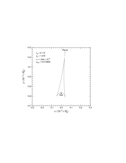
Figure 14: Model A of event MACHO 98–BLG–35 viewed in the source plane. The ”stealth-bomber” shaped line is the ”caustic” or locus of points where a point source would be infinitely magnified by the lens system. The source star moves horizontally left-to-right through the origin. The coordinate units in the source plane are projected Einstein radii, i.e. $R^{\prime}_{\rm E}=(D_{\rm OS}/D_{\rm OL})\times R_{\rm E}$. For any source radius $\leq 6R_{\odot}$, the source star does not intersect the caustic. Rhie & Bennett (1996), Rhie (1999), and Rhie et al (1999) discuss further examples of events with similar caustic geometries, and also the origin of the stealth-bomber terminology.

In Fig. 14, we depict an additional view of model A, this time in the source plane. This shows the contour of infinite magnification for the event (i.e. the “caustic”). It is seen that the source star does not pass between the star and the planet. Hence the perturbation is negative as can be seen in Fig. 12. It is also seen that the source star does not intersect the caustic at any time.

Rhie et al. (2000) estimated a radius of 1–3$R_{\odot}$ for the source star in this event. We have repeated the above $\chi^{2}$ minimization process for model A using a source radius of 0.004$R_{\rm E}$($\approx 2R_{\odot}$). We obtain best fit values for the planetary parameters of $\epsilon=1.3\times 10^{-5}$ at position $(0.08,1.17)$ with $\Delta\chi^{2}=36.1$. The effect of increasing the source size serves to partially wash out the fine structure in the microlensing light curve near the peak. The improvement in $\chi^{2}$ is then not as good as those for smaller source radii. These results indicate a likely source star radius $\la 2R_{\odot}$.

Figure 10: Coordinate system used to analyse light curves in terms of planets orbiting a lens star. The coordinates scales are in units of the Einstein radius $R_{\rm E}$.

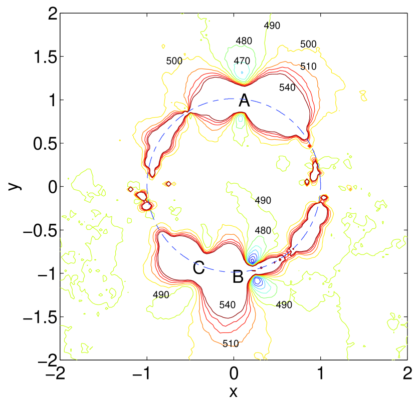
Figure 11: Map of $\chi$-squares of the data for MACHO 98–BLG–35 by the MOA, MPS and PLANET groups for an Earth-mass planet ($\epsilon=10^{-5}$) orbiting the lens star at projected radii up to $2R_{\rm E}$. The coordinate system is the same as in Fig. 10. There are three minima interior to the ring, and three corresponding minima exterior to the ring, labeled A, B and C respectively. These are the possible positions of terrestrial-mass planets orbiting the lens star at the time of the microlensing event. Planet positions of higher likelihood were determined by allowing the planet-to-lens mass fraction to vary from $10^{-7}$ to $10^{-3}$ and locating deeper $\chi^{2}$ minima.

Table 3: Parameters and statistics of the best planetary fits to the combined data of the MOA, MPS and PLANET groups from $-t_{\rm E}$ to $+t_{\rm E}$ for MACHO 98–BLG–35. Model O is the best fit without a planet. The $\Delta\chi^{2}$ values are the normalized values with respect to model O. The coordinate system is as depicted in Fig. 10. The planetary mass fraction, $\epsilon$, is in units of $10^{-5}$. For each set of planetary coordinates, an alternative set is possible with a planet of the same mass at the inverse radius. For model A, for example, the conjugate coordinates are (0.07,0.82,1.3).

Model	Planet A			Planet B			Planet C			$t_{\rm max}$	$t_{\rm E}$	$u_{\rm min}$	$\Delta\chi^{2}$
	$x_{\rm p}$	$y_{\rm p}$	$\epsilon$	$x_{\rm p}$	$y_{\rm p}$	$\epsilon$	$x_{\rm p}$	$y_{\rm p}$	$\epsilon$
O	-	-	-	-	-	-	-	-	-	999.1494	20.37	0.013829	0
A	0.11	1.22	1.3	-	-	-	-	-	-	999.1506	20.32	0.013829	60.0
B	-	-	-	0.30	$-$1.11	2.8	-	-	-	999.1499	20.31	0.013964	34.5
C	-	-	-	-	-	-	$-$0.37	$-$0.86	0.17	999.1493	20.33	0.013898	13.7
A+B	0.16	1.25	0.79	0.35	$-$1.14	2.8	-	-	-	999.1499	20.27	0.013837	41.7
B+C	-	-	-	0.30	$-$1.12	2.6	$-$0.34	$-$0.86	0.19	999.1500	20.33	0.013978	57.5
A+C	0.15	1.21	0.99	-	-	-	$-$0.33	$-$0.84	0.18	999.1508	20.30	0.013857	47.2
A+B+C	0.19	1.28	0.30	0.34	$-$1.15	2.9	$-$0.35	$-$0.87	0.17	999.1490	20.34	0.013847	56.1

Model B may be seen to correspond to the one previously found by Rhie et al. (2000) on the basis of DoPHOT analyses of the MPS and MOA datasets. The inclusion of the PLANET dataset has served to lower the planetary mass-fraction of this model from $7.0\times 10^{-5}$ to $2.8\times 10^{-5}$. Model B+C may be considered a generalization of the original model of Rhie et al. (2000) to which a second, nearby, very-low-mass planet has been added. The inclusion of a second planet as in model B+C gives a significant decrease in $\chi^{2}$ over the single planet model B with $\Delta\chi^{2}=30.0$. While model A is the simplest, we have included model B+C to illustrate the potential of microlensing to map multi-planet systems..

Thus far the discussion has been in terms of $\Delta\chi^{2}$ values because these are both convenient for comparing different models, and because they are less sensitive than absolute $\chi^{2}$ values to the uncertainties in the measurements. Visual inspection of Figs. 7 and 12 shows that model O is not a good fit to the data, and that model A is significantly better. Assuming that model A is actually correct, a likelihood for model O may be estimated by forcing the $\chi^{2}$ of model A to be the same as the number of degrees of freedom by renormalizing all the errors by a constant factor. This yields $\chi^{2}=358.0$ with 298 degrees of freedom for model O which corresponds to a deviation of $2.5\sigma$ for which the probability is $<1$%. A more satisfactory procedure for interpreting MACHO 98-BLG-35 would be to analyze all the datasets using difference imaging, determine all the errors self-consistently, and redo the planetary modelling.

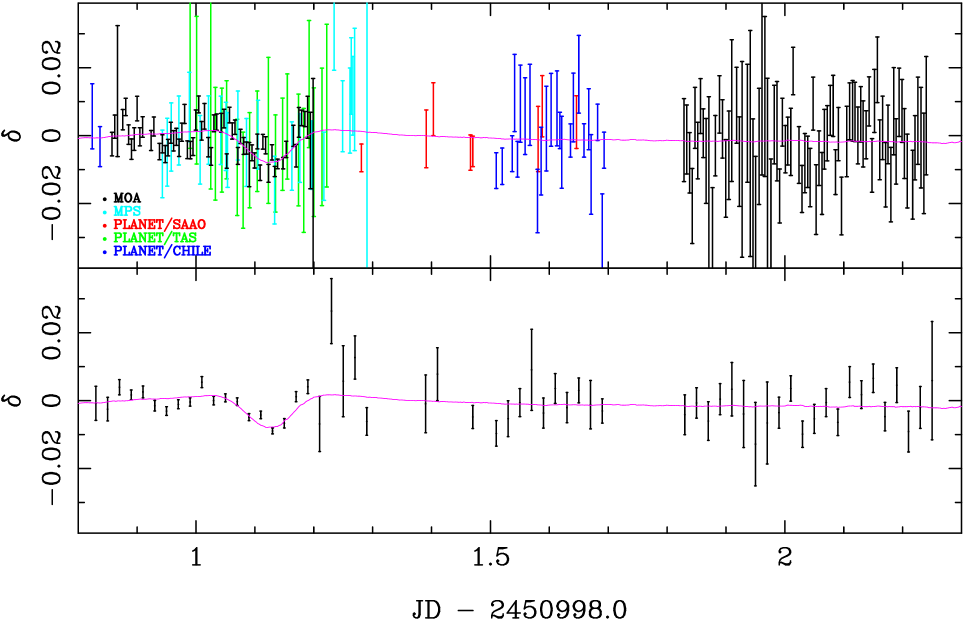
Figure 12: Light curve for the single planet model ”A” of event MACHO 98–BLG–35 together with the data of the MOA, MPS and PLANET groups. The top figure shows all the data while the lower figure shows the data binned and weight averaged on 0.02 day intervals. The quantity $\delta$ is the fractional deviation of the fit from the lensing star component of the star$+$planet system. The dip in the light curve at around day 1.1 is seen in the MOA, MPS and PLANET data.

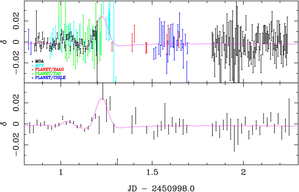
Figure 13: Same as Fig. 12 but for the two planet model B+C.

For the two planetary configuration models that we favour here, model A and model B+C, the renormalized $\Delta\chi^{2}$ was around 60 and the number of degrees of freedom were around 290. Gaudi et al (2002) subsequently proposed setting an alternative detection threshold for low-mass planets, namely $\Delta\chi^{2}>60$ irrespective of the number of degrees of freedom. Howver, as the chance probability depends on the number of degrees of freedom, we advocate consideration of this factor. Gaudi et al also noted that heavy planets should be detected before light planets unless the planetary mass function is steep. We note that, in the absence of observational information on the planetary mass function, a steep function cannot be excluded. Gaudi et al analysed PLANET data for several microlensing events, including MACHO 98–BLG–35, and reported no evidence for planets. Our representation of their data in Figs. 12 and 13 is consistent with this. However, it is clear from Figs. 12 and 13 that the PLANET data, derived using profile fitting photometry, are not in conflict with the MOA data, derived using the more precise image subtraction photometry. As such the PLANET data do not rule out the planetary models we considered in our study.

Exclusion regions for giant planets orbiting the lens star of MACHO 98–BLG–35 were also computed using the inverse ray shooting technique. The $\chi^{2}$ maps for one-planet models for mass ratios of ($\epsilon=2.8\times 10^{-3}$), ($\epsilon=8.5\times 10^{-4}$) and ($\epsilon=1.3\times 10^{-4})$ were computed. These correspond to Jupiter, Saturn, and Uranus mass planets orbiting a one third solar mass star. The contours were found where $\chi^{2}$ exceeds its value for the single lens model by 90. This value was chosen, under the assumption that any excluded model should have $\sim 20$ or more consecutive measurements deviating systematically by $(1-2)\sigma$ or more from it. This threshold would appear conservatice when compared with the $\Delta\chi^{2}$ values for the planetary models. The higher value was chosen to allow for the fact that the other parameters $t_{\rm max}$, $t_{\rm E}$, and $u_{\rm min}$ were not allowed to float but were fixed at the single lens model values in this computation. The exclusion regions so obtained are shown in Fig. 15. It is clear that a large region surrounding the lens star of MACHO 98–BLG–35 is devoid of gas-giants like Jupiter or Saturn. Jovian planets with projected radii $\sim$0.2–15 $R_{\rm E}$ or $\sim$0.4–30 AU are excluded. A similar result was found previously by Rhie et al. (2000), but the inclusion of further data and the use of subtraction photometry have served to enlarge the exclusions regions.

5.2 MACHO 99–LMC–2

The microlens event MACHO 99-LMC-2 was unusual in that it is the only high magnification event observed to date that occurred towards the Magellanic Clouds. It was found independently by both the MACHO and the OGLE groups. It was included in the observing program of the MOA group because it afforded an opportunity to search for a planet in an external galaxy, i.e. for an extra-galactic planet, under the assumption that the event is an example of the “self-lensing” process of Sahu (1994). In this process, a foreground star in the LMC lenses a background star in the LMC. We note, however, that the question of the most likely location of lenses observed towards the LMC has not yet been settled (see, for example, Alves & Nelson 2000, Alcock et al. 2001).

The typical value of the Einstein radius for self-lensing is the same as for galactic bulge events, i.e. $\sim 2$ AU. This follows from Eqn. 1 assuming a typical lens mass $\sim 0.3M_{\odot}$ and values of order 48 kpc, 2 kpc and 50 kpc for $D_{\rm OL}$, $D_{\rm LS}$ and $D_{\rm OS}$. Consequently, high magnification events observed towards the LMC offer similar prospects for planet detection as they do towards the galactic bulge.

The data for MACHO 99-LMC-2 which are displayed in Fig. 8 and Table. 2 show no clear evidence for a deviation from the light curve of a single lens. Consequently, only exclusion regions for giant planets surrounding the lens were computed. This was done with the procedure used above for MACHO 98–BLG–35. The exclusion regions so obtained are displayed in Fig. 16. Jovian planets with projected radii $\sim$0.4–10 AU are excluded. These results are, to our knowledge, the first limits placed on planetary companions to an extra-galactic star.

5.3 OGLE 00-BUL-12

The data on OGLE 00-BUL-12 in Fig. 9 and Table 2 show possible evidence of a deviation from the behaviour of a single lens. Consequently, they were subjected to the same analysis as that accorded to MACHO 98–BLG–35. The initial search with the super-cluster computer yielded several possible planetary models, but none of these were statistically significant improvements over the single lens fit. However, one of them showed interesting behaviour, and this is reproduced below in Figs. 17 and 18 to illustrate the potential of the high magnification technique.

The light curve shown in Fig. 17 shows the characteristic double-spiked behaviour of a caustic crossing. This is illustrated in Fig. 18 which shows the source plane view of the model. Here a source radius of $1R_{\odot}$ has been assumed. The combination of high magnification and caustic crossing occurring simultaneously in one event leads to enhanced sensitivity for planet detection. The planetary mass-fraction for the light curve in Fig. 17 ($\epsilon=0.055\times 10^{-5}$) corresponds to a planet of mass similar to that of Mercury orbiting a one-third solar mass star. The improvement over the single lens fit corresponds to $\Delta\chi^{2}=13.7$. We note that further data were obtained during the peak of this event (Sackett 2001). These could be analysed by the image subtraction technique and included in a future analysis of the event, thus reducing the uncertainties in the present analysis.

Given the limited coverage of this event and the low statistical significance, we do not present this as a planetary detection. However, the analysis raises interesting possibilities. The striking feature of this event is its very high peak magnification of about 160. Light curves such as that shown in Fig. 17 for a Mercury mass planet should apply to other events with similarly high magnifications. It can be seen that such planets can produce deviations from the single lens by about 1%. Such deviations should be detectable by a network of 1-m class telescopes providing continuous and complete coverage of the peaks of high magnification events.

Exclusion regions for gas-giant planets orbiting the lens of OGLE 00-BUL-12 were also computed. These are shown in Fig. 19. Jovian planets with projected radii $\sim$0.2–30 AU are excluded.

Figure 15: Exclusion regions for giant planets similar to Jupiter, Saturn and Uranus orbiting the lens star of event MACHO 98–BLG–35. The coordinate system is the same as in Fig. 10. The reflection symmetry about the Einstein ring that is discussed in §5.1 is evident.

6 Discussion and Conclusion

The original proposal of Griest & Safizadeh (1998) to study extra-solar planets in gravitational microlensing events of high magnification has received support from the present work. It has been demonstrated that terrestrial-mass planets at orbital radii $\sim 2$ AU may be detected with 1-m class telescopes. The essential requirement is the relentless observation of the peaks of high magnification events with coordinated telescopes encircling the globe, a relatively straightforward task. The dense stellar fields in which microlensing is necessarily observed require special photometric techniques to take account of the blending of stellar images. Difference imaging analysis appears to be well suited to this task.

If a concerted effort was made by the microlensing community to detect and monitor relentlessly future events of high magnification, it could reasonably be anticipated that a first approximate measurement of the abundance of terrestrial planets could be obtained in a few years. If $\sim 10$ high magnification events can be detected per year, a rough measurement or upper limit on the abundance of Earth-mass planets orbiting $\sim$0.3$M_{\odot}$ stars at projected radii $\sim$1.5–2.5 AU could be obtained in a few years (Bond et al 2002). As demonstrated here, one might also obtain new information on planets as light as Mercury, on extra-galactic planets, and on gas-giants. Also, multi-terrestrial-planet systems should be able to be mapped in some cases (Rattenbury et al 2002), rather like the multi-gas-giant systems presently being mapped by the radial velocity community (Butler et al. 1999). Ultimately, a dedicated wide-angle space-borne telescope such as that planned for the proposed GEST mission would provide excellent sensitivity towards all solar-system analogues except Mercury and Pluto (Bennett et al 2002).

It appears likely that none of the three lens objects studied here contains a Jovian planet. This is consistent with previous measurements by Marcy & Butler (1998) and of Albrow et al. (2001) of other systems. The dearth of Jupiter-like planets enhances the sensitivity of microlensing studies of terrestrial planets, merely through the lack of “background” signals from gas-giants.

For all three events further data by microlensing groups exist that could be analysed using image subtraction and incorporated in the planetary modeling. This could be expected to produce results of greater precision, and to diminish ambiguities that presently exist in the planetary modeling.

The assumptions made in the present analysis on the masses, sizes and distances of the lens and source stars may be able to be avoided in the future. When the Next Generation Space Telescope comes into operation, and as the lens and source stars in today’s microlensing events begin to diverge, it should be possible to measure the lens and source stellar parameters in these events by elementary photometry (Rattenbury et al 2002). This being the case, the planetary modeling would be entirely free of undetermined parameters

Figure 16: Exclusion regions for gas-giants similar to Jupiter, Saturn and Uranus orbiting the lens star of event MACHO 99-LMC-2. The coordinate system is the same as in Fig. 10.

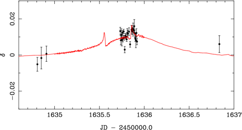
Figure 17: Light curve around the peak of OGLE 00-BUL-12 for the best low mass planet model fit together with the photometry measurements derived from image subtraction. The jaggedness throughout the model curve is small amplitude computational noise.

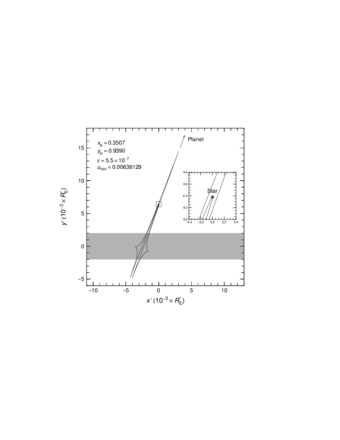
Figure 18: Planetary model of event OGLE 00-BUL-12 that includes an arrow-like caustic. The axes are as in Fig. 14. The source star moves horizontally left-to-right through the origin, and thus intersects the caustic whatever its radius. The shaded region corresponds to the track of a source star of radius of $1R_{\odot}$. Similar arrow-like caustics appear in Wambsganss (1997).

We conclude that coordinated observations using 1-m class telescopes of gravitational microlensing events of high magnification are capable of making valuable contributions to the study of planets orbiting other stars.

Figure 19: Exclusion regions for gas-giants similar to Jupiter, Saturn and Uranus orbiting the lens star of event OGLE 00-BUL-12. The coordinate system is the same as in Fig. 9. The outer extremities of the exclusion region for a Jupiter analogue are given by the reflection symmetry $a\sim 1/a$.

References

- [1] Abe, F., et al., 1997, in “Variable Stars and the Astrophysical Returns of Microlensing Surveys”, eds. R.Ferlet, J. Maillard, and B. Raban, Editions Frontieres, France, p. 75.
- [2] Albrow, M.D., et al., 2001, ApJ, 556, L113
- [3] Alard, C., Lupton R., 1998, ApJ, 503, 325
- [4] Alard, C., 1999, A&A, 342, 10
- [5] Alcock, C., et al., 2001, ApJ, 552, 582
- [6] Alves, D., Nelson C., 2000, ApJ, 542, 789
- [7] Bennett, D.P. et al., 2002, in AAS 199th meeting, Washington DC
- [8] Bennett, D.P., et al., 1999, Nat., 402, 57
- [9] Bennett, D.P., Rhie S.H., 1996, ApJ, 472, 660
- [10] Bolatto, A.D., Falco, E.E., 1994, ApJ, 436, 112
- [11] Bond, I.A., et al., 2002, submitted to MNRAS
- [12] Butler, R.P., Marcy, G. W., Fischer, D. A., Brown, T. M., Contos, A. R., Korzennik, S. G., Nisenson, P., Noyes, R. W., 1999, ApJ, 526, 916
- [13] Charbonneau, D., Brown, T. M., Latham, D. W., Mayor, M., 2000, ApJ 529, L45
- [14] Gaudi, B.S. et al., 2002, astro-ph/0104100, ApJ, in press
- [15] Gould, A., Loeb A.,1992, ApJ, 396, 104
- [16] Griest, K., Safizadeh N., 1998, ApJ, 500, 37
- [17] Henry, G.W., Marcy, G.W., Butler, P., Vogt, S., 2000, ApJ, 529, L41
- [18] Jha, S., Charbonneau, D., Garnavich, P. M., Sullivan, D. J., Sullivan, T., Brown, T. M., Tonry, J. L., 2000, ApJ, 540, L45
- [19] Liebes, S., 1964, Phys. Rev., 133, B835
- [20] Mao, S., Paczynski B., 1991, ApJ, 374, L37
- [21] Marcy, G.W., Butler R.P., 1998, ARA&A, 36, 57
- [22] Mayor, M., Queloz D., 1995, Nature, 378, 355
- [23] Paczynski, B., 1986, ApJ, 304, 1
- [24] Perryman, M.A.C., 2000, Rep. Prog. Phys., 63, 1209
- [25] Rattenbury, N.J., Bond, I.A., Skuljan, J., Yock, P.C.M., 2002, MNRAS, submitted
- [26] Rhie, S.H., 1999, in Gravitational Lensing: Recent Progress and Future Goals, 25-30 July 1999, Boston University
- [27] Rhie, S.H., Becker, A. C., Bennett, D. P., Fragile, P. C., Johnson, B. R., King, L. J., Peterson, B. A., Quinn, J, 1999, ApJ, 522, 1037
- [28] Rhie, S.H., Bennett, D.P., 1996, Nucl. Phy. Supp., 51B, 86
- [29] Rhie, S.H. et al., 2000, ApJ, 533, 378
- [30] Sackett, P.D., 2001, in Planetary Systems in the Universe: Observations, Formation, and Evolution, ASP Conf. Series, eds A.J. Penny, P. Artymowicz, A.-M. Lagrange, and S.S. Russell, in press
- [31] Sahu, K.C., 1994, Nature, 370, 275
- [32] Schechter, P., Mateo M., Saha A., 1993, PASP, 105, 1342
- [33] Udalski, A., Kubiak M., Szymanski M., 1997, AA 47, 319
- [34] Wambsganss, J., 1997, MNRAS, 284, 172
- [35] Yanagisawa, T., et al., 2000, Exp. Astron., 10, 519