Real-Time Difference Imaging Analysis of MOA Galactic Bulge Observations During 2000

Abstract

We describe observations carried out by the MOA group of the Galactic Bulge during 2000 that were designed to detect efficiently gravitational microlensing of faint stars in which the magnification is high and/or of short duration. These events are particularly useful for studies of extra-solar planets and faint stars. Approximately 17 deg² were monitored at a sampling rate of up to 6 times per night. The images were analysed in real-time using a difference imaging technique. Twenty microlensing candidates were detected, of which 8 were alerted to the microlensing community whilst in progress. Approximately half of the candidates had high magnifications ($\ga 10$), at least one had very high magnification ($\ga 50$), and one exhibited a clear parallax effect. The details of these events are reported here, together with details of the on-line difference imaging technique. Some nova-like events were also observed and these are described, together with one asteroid.

1 Introduction

The observation of gravitational microlensing events is becoming established as an important tool in several astrophysical endeavours. These include the search for extra-solar planets, studies of dark matter, studies of stellar atmospheres, and studies of galactic structure. More than 500 microlensing events, most of them alerted in real time, have been identified by the microlensing survey groups MACHO [1993], OGLE [1992], and EROS [1993]. These groups monitored some millions of stars within their fields of view to find the microlensing events. The photometry measurements were based on profile fitting software such as Dophot [1993] which determines fluxes by integrating over the profile of a given star on a given image.

While profile fitting techniques have proved to be highly successful, the limitations of this type of analysis have been recognized for some time. The most serious limitation is the contamination of flux measurements by the “blending” of the profiles of neighbouring stars. This problem becomes more serious when one encounters crowded regions of stars within the fields of view. Blending causes systematic errors in photometry measurements and subsequent systematic errors in the determination of microlensing parameters such as event duration and peak amplification [1998]. Alard [2001] has shown that, using an image subtraction or difference imaging analysis (hereafter DIA) to allow for the effects of blending, an unbiased reconstruction of the mass function in the Galactic bulge should be possible using microlensing data alone.

Another problem with profile fitting analyses is that only those microlensing events whose source stars are visible and resolvable at baseline are detected. Microlensing events that rise from below the observational threshold to be visible during times of high magnification are missed. This is unfortunate, because these events with faint source stars are potentially capable of providing valuable information. The mere detection of faint stars in the Galactic Bulge that are normally undetectable can clearly provide useful information. For example, if the magnification is high, spectroscopic information may also be obtained that is not available otherwise (Lennon et al. 1996, 1997; Minniti et al.1998). Kane and Sahu (2001) recently made a kinematic study of the far side of the Galactic bulge using spectroscopy of microlensed sources.

The peaks of high magnification events provide valuable information on extra-solar planetary systems. Griest and Safizadeh (1998) showed that the probability for detecting Jupiter-like planets is nearly 100% for events with peak amplifications $\ga 100$ provided good photometric sampling is carried out around the times of the peaks, and that the probability for detecting Earth-like planets is substantial. They also showed the probability for detecting Jupiter-like planets is substantial in events with peak amplifications $\ga 10$. These predictions have been borne out by observation (Rhie et al. 2000; Albrow et al. 2000; Bond et al. 2001). As will be shown here, high magnification events can be detected efficiently using DIA.

DIA largely overcomes the problems caused by blended or undetected microlensing source stars. Recent re-analyses of the MACHO database using DIA have increased the microlensing detection rate and improved the quality of the photometry (Alcock et al. 1999a; 1999b; 2000). A re-analysis of the OGLE database is underway and similar results are emerging [2000]. All of these analyses were carried out off-line.

During 2000 we applied DIA to observations of the Galactic Bulge carried out by the MOA Group. The analysis was “real-time” in that alerts of microlensing events in progress were provided to the microlensing community. In this paper we describe our implementation of the real-time DIA method and present the transient phenomena observed during 2000.

2 Observations by MOA of the Galactic Bulge

The observations were carried out using the 60-cm Boller & Chivens telescope of the Mt John University Observatory in New Zealand. The telescope was modified by the MOA group to provide a 1$\aas@@fstack{\circ}$3 field of view at f/6.25 and to enable computer controlled tracking (Abe et al. 1997). The data were taken using the wide field camera, MOA-cam2, that was constructed by the MOA group [2000]. MOA-cam2 is a mosaic camera comprised of three abutted thinned 2k$\times$4k SITe CCD chips. Two wide passbands were employed: a “blue” (400–630 nm) and a “red” (630–1000 nm) band. The wide passbands compensate for the small telescope aperture. The total field of view over the three CCDs is $55\arcmin\times 83\arcmin$ and the pixel size on the sky is $0.81\arcsec$. This is matched to the less than ideal seeing of the set-up which ranges from about $1.8\arcsec$ to $3.5\arcsec$, with the median at about $2.5\arcsec$. These are global figures that include dome seeing, etc.

The observational strategy employed by MOA for the Galactic Bulge in 2000 was somewhat different from that of the established survey groups MACHO, OGLE, and EROS. Rather than sample a large area of the Bulge once per night, we chose to sample a smaller area several times per night. This decision was taken mainly with the aim of improving our sensitivity to very high magnification events which are expected to rise and fall very rapidly and only be detected above the observation threshold for a few days or less.

For the 2000 observations, a total of 14 MOA-cam2 fields towards the Galactic Bulge were selected on the basis of the distribution of microlensing events detected by the MACHO Collaboration during 1995–1999. These fields cover an area of $\sim 17$ deg². The exposure time was 180 seconds per field with most exposures being taken in the red passband. Exposures in the blue passband were only made occasionally and are not used in this study. This observational strategy allowed a sampling rate for the full 14 fields of up to 6 times per night. These fields were observed by MOA between 2000 March and September. Problems with the camera electronics prevented observations over a six-week period during July–August.

3 Data Analysis

3.1 Image Subtraction Method

Figure 1: Difference imaging in action. The top left image is a sub-region of a reference image. The top right image is a corresponding observation image. The squares in the two top images mark the location of stamps used to calculate the kernel. The lower left image is the result of subtracting the reference image from the observation image. The lower right image is the same subtracted image with the positions of saturated stars masked out.

Two geometrically aligned images taken under conditions of different seeing are related through the convolution relation

$$i(x,y)=r*k(x,y)+b(x,y).$$ (1)

Here $r$ is the better seeing image referred to as the “reference” image and $i$ is the current “observation” image. The convolution kernel $k$ encodes the seeing differences and $b$ represents the sky background differences between the two images. Solving for the convolution kernel is the crucial step in image subtraction. There are two approaches in use for doing this. One matches point spread function (PSF) models on the two images by solving for the kernel in Fourier space (Phillips & Davis 1995; Tomaney & Crotts 1996). This approach was adopted by Alcock et al. [1999a] in their re-analysis of a subset of the MACHO data.

The other approach is to directly model the kernel in real space [1998]. We developed our own implementation of this method. This includes the modification of Alard [1999] that models spatial variations of the kernel across the CCD. The mathematical techniques are described fully by Alard & Lupton [1998] and Alard [1999]. Here we summarize our implementation. The convolution kernel function at a given location $(x_{0},y_{0})$ is expressed as a linear combination of analytical “basis” functions

$$k(x_{0},y_{0},x,y)=a_{0}f_{0}(x,y)+\sum_{m}a_{m}(x_{0},y_{0})f_{m}(x,y).$$ (2)

The coefficients in the linear combination are spatially dependent. They are also modeled as a linear combination of basis functions which takes the form of a two dimensional polynomial

$$a_{m}(x_{0},y_{0})=\sum_{n}a_{mn}x_{0}^{p}y_{0}^{q},$$ (3)

where the polynomial indices $p$ and $q$ depend implicitly on the function index $n$. The basis functions used to model the kernel take the form of a combination of two dimensional Gaussian functions and polynomials. The function $f_{m}(x,y)$ in Eqn. 2 can be expressed in such a way as to render the integral of each but the first basis function zero. Consequently the integral of the kernel itself is constant across the chip regardless of the spatial variations of the kernel. The differential background is modeled in the same way as the spatial variations in the kernel:

$$b(x,y)=\sum_{n}b_{n}x^{p}y^{q}$$ (4)

where again the polynomial indices depend implicitly on the function index.

The solution for the coefficients ${a_{mn}}$ and ${b_{n}}$ may be found using standard linear techniques. The linear system is constructed using a number of sub-regions, referred to as “stamps”, centred on bright, but not saturated, stars throughout the image. An advantage of this method of solution is that these stamps need not be centred on isolated stars with clear point spread functions (PSF stars). There can be any number of stars to any degree of crowding within a stamp. However, we impose the strict requirement that regions enclosed by the stamps, plus an additional margin given by half the kernel size, are completely free of bad pixels including dead columns and bleeding columns due to nearby saturated stars. Imposing this condition greatly improves the robustness in obtaining good quality subtracted images. Another consideration is that the size of the linear system is large when one includes the spatial variations in the convolution kernel. The computing time required to calculate the linear system can be greatly reduced using an accelerated summation procedure which assumes that the kernel is constant within individual stamps [1999].

Our implementation of the kernel solution method along with the subsequent image subtraction is coded in C++. It is worth mentioning here the merits of using an object oriented programming language for this purpose. Eqns. 2–4 are somewhat unwieldy to encode in a procedurally oriented language such as Fortran or C. The object oriented feature of C++ allows one to encapsulate neatly a set of basis functions and their associated polynomial index tables in a single class. One then declares separate class instances for each set of basis functions describing the kernel, its spatial variations and the differential background.

The PSF profiles are known to vary across the field for large CCD images. Consequently, the possible spatial variation of the convolution kernel is an important consideration. The approach adopted by the MACHO collaboration was to divide their images into small sub-rasters and solve for the convolution kernel separately on each of these sub-rasters assuming no significant variations in the kernel occurred on their length scales [1999a]. However, for the MOA images, we find small but significant spatial variations of the kernel even over small $500\times 500$ sub-regions of the field. This prompted us to select the direct kernel modeling method which can easily model these spatial variations.

Another consideration which influenced our choice of kernel solution method was that the PSF matching method requires high signal-to-noise empirical PSF models on both the reference and observation images. This would be difficult to achieve consistently using a small telescope such as ours at a site with only moderately good seeing. On the other hand, the direct kernel modeling method only requires the reference image to be of high signal-to-noise.

An example of a subtracted image is shown in Fig. 1. The approach taken to subtract a MOA 2k$\times$4k observation image from its corresponding reference image involved first selecting suitable stamps on the reference image. Typically $\sim 400$ stamps were selected per 2k$\times$4k field. An observation and reference image were then tiled into 1k$\times$1k sub-images which were small enough to allow the spatial variations in the kernel and differential sky background to be satisfactorily modeled using smooth functions. The solution for the convolution kernel and its associated spatial variations, together with the differential sky backgrounds, was computed for each sub-region. The corresponding subtracted image was then formed using

$$\Delta i(x,y)=i(x,y)-r*k(x,y)-b(x,y)$$ (5)

For a time series of observation images of a given field, a reference image was formed from the best seeing image or a combination of the best seeing images. The reference image is fixed over the entire time series. The stamps used for the kernel solution were also fixed for the time series of observations.

A mask image mapping the distribution of saturated stars was also formed from the reference image. If a particular star contained saturated pixels, the entire star profile was masked out. There is little useful data that can be obtained at the position of saturated stars. The mask was applied to all subtracted images to obtain final images.

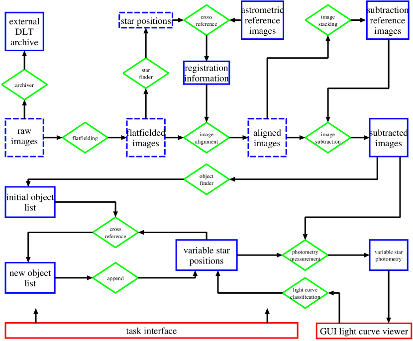
Figure 2: Road map of the on-line data analysis environment. The boxes represent the various databases. The dashed boxes datasets which are flushed periodically to relieve pressure on system disk space. The diamonds represent the analysis procedures connecting the databases.

3.2 Data Analysis Environment

In this work, two distinct modes of analysis were employed. The “online” analysis mode was used for real time reductions the large quantity of 2K$\times$4K images collected during observations. A more detailed and rigorous “follow-up” analysis was then applied to individual events found in the online analysis. The online analysis system is shown schematically in Fig. 2. The process involves the interplay of a large number of image and numerical datasets. It is more helpful to regard the system as a data and image management system rather than a linear data reduction “pipeline”. The key features of the analysis system are as follows.

3.2.1 Task Interface

Each of the tasks linking the databases shown in Fig. 2 is controlled by a single Perl script. These scripts function as wrappers to lower level image and data analysis programs most of which are coded in C++. Each task can be run individually or combined in other scripts to provide a higher layer of automation. This design provides considerable flexibility in operation, ranging from complete automation down to image-by-image interaction.

3.2.2 Image Registration

The image registration database provides information on the geometric alignment of observation images to their corresponding astrometric reference images. The registration process involves cross-referencing resolved stars on the two images to achieve alignment. Each of the 2k$\times$4k observation images was sub-divided into 1k$\times$1k sub-frames. The brightest 1000 stars within each sub-region were found using our implementation of the algorithm in the IRAF task DAOFIND. The star positions in each sub-frame were cross-referenced with star positions on the corresponding sub-frame of the astrometric reference using a smart algorithm which starts with the pre-supposition that the brighter stars on the observation image will be correspondingly bright on the astrometric reference image. A slower but very robust alternative algorithm was used as a backup if necessary. This combination of algorithms provided an extremely robust frame-to-frame matching procedure that worked for all images taken under a variety of viewing conditions. For each observation image one finally obtained a list of 6000–8000 cross referenced stars over the full 2k$\times$4k field. The positions of these stars on the observation and reference images were entered into the registration database.

3.2.3 Image Alignment

Geometrically aligned images were formed from flat-fielded images using information in the registration database. The alignment task was controlled by a Perl wrapper script for the IRAF tasks GEOMAP and GEOTRAN. This alignment process was used in the construction of subtraction reference images and in preparing images for the subtraction process itself.

3.2.4 Reference Image Databases

These databases contain the astrometric and image subtraction reference images for each CCD of each observation field. The astrometric reference images define the coordinate system to which all observation images were geometrically aligned. The images used for both astrometry and subtraction were selected from amongst the best seeing, highest signal to noise, and lowest airmass images obtained early in the 2000 Galactic Bulge observation season.We decided not to form subtraction reference images by combining several images. Instead we chose just one good seeing image per field as the reference. When combining large images such as ours, there is a danger of corrupting the linearity in the final image due to non-uniformities in the sky background across the chip. In image subtraction, it is crucial that the pixel values associated with the images are linear with respect to the incident flux..

3.2.5 From Raw to Subtracted Images

The backbone of the image reduction flow involves processes that generate subtracted images from raw observation images. Intermediate image databases contain flat-fielded and aligned images. To relieve pressure on computer disk space, raw, flat-fielded, and aligned image databases were flushed periodically. However, all raw images were externally archived onto DLT tapes. When required, a given set of flat-fielded and aligned images could easily be regenerated using information in the registration database. On the other hand, all subtracted images were retained on disk as these were constantly being accessed by the photometry measurement processes.

3.2.6 Identifying Objects on Subtracted Images

The positions of variable stars on a given subtracted image exhibited positive or negative profiles depending on whether the flux had increased or decreased relative to the reference image. The subtracted images also contained spurious profiles not associated with stellar variability. One type of spurious profile arose from the effects of differential refraction. Dependent upon the star’s colour and the airmass at the time of observation, the position of its centroid was sometimes displaced to a greater extent than other stars. The result was an imperfect subtraction at the star’s position, giving a combined positive and negative profile. We did not attempt to correct for this effect, but instead filtered out these imperfect subtractions (see Alcock et al. 1999b for a discussion on how to deal with differential refraction).

The first step in identifying objects associated with genuine variability was the application of the star finding algorithm described previously to the subtracted image to produce an initial list of variable star positions. This list was then screened by applying a second algorithm which examined the profile at each position. Essentially, if the profile contained a large number of either positive definite or negative definite pixel values, then the profile was deemed to be that of a genuine variable star. For each CCD on each field, newly detected objects were assigned running numbers according to discovery sequence.

3.2.7 Photometry Databasing

We did not maintain a database of light curves of all resolved stars across the observation fields. Rather, we maintained a database of variable star positions coupled with the database of subtracted images. Light curves were calculated only for objects of “current interest” such as newly identified transient events. The variable star position database was updated periodically as new variables were identified and more refined positions were calculated. Since the subtracted images were retained on disk, a light curve at any given set of positions could be easily generated. In the online analysis, we extracted photometric measurements from the subtracted images using aperture photometry with an aperture radius of 6 pixels. In the follow-up analysis described in the next section, we used more a precise measurement technique.

3.2.8 Event Selection

We wished to detect new transient events online as opposed to periodic variables such as Miras, RR Lyrae stars, etc. A search for new events was generally carried out at the end of each night of good seeing conditions. For each field, the sequence of subtracted images from the previous night was combined to form a mean subtracted image which was examined for positive and negative profiles due to stellar variability. The positions of these profiles were cross-referenced with those of variable stars previously detected to produce a list of “new” variables. The variable star database was then updated by appending the new detections. Light curves for the new detections were generated by performing aperture photometry at their respective positions on the entire sequence of subtracted images up to the current observation date. This practice of periodically carrying out new searches for events rendered the procedure sensitive to short timescale transient events.

The light curves corresponding to all new detections were scrutinized by eye using a graphical tool. If a particular light curve was clearly characteristic of periodic stellar variability, the associated position was flagged as hosting a “variable” star. On the other hand, if a light curve exhibited behaviour characteristic of a microlensing candidate or other transient event, it was flagged as “interesting”. The interesting events were further scrutinized by examining both the subtracted and unsubtracted images at their respective positions and checking for bad pixels, nearby saturated stars, bleeding columns etc. Interesting events were closely monitored throughout the viewing campaign. If any event could be clearly identified as a microlensing candidate or another tyoe of interesting transient event, a MOA Transient Alert was issued to the microlensing community and posted on the World Wide Web.

Early in the observation season, the number of light curves to inspect by eye was large but this number decreased rapidly as more and more periodic variables were flagged. As the observation season progressed, around 100–150 previously undetected objects were found each time a search for new events was carried out. This number of corresponding light curves could easily be scanned by eye and classified. There is merit in being able to pick up events by eye in real time. No assumptions on the form of the variability of transient events need be made in the selection process. As well as microlensing events, the possibility of detecting new and unusual transient phenomena arises with such a system.

3.2.9 Computational Constraints

Table 1: Summary of All Detected Transient Events

MOA ID			Coordinates (J2000.0)		Alert Status
Field	CCD	ID	RA	Dec	MOA	OGLE
ngb1	2	2667	17:54:56.68	$-$29:31:47.5	2000–BLG–7
ngb1	2	2717	17:57:07.91	$-$29:09:59.3	2000–BLG–11
ngb1	3	727	17:54:29.77	$-$28:55:59.3	2000–BLG–3
ngb1	3	2540	17:58:20.94	$-$28:47:48.8
ngb1	3	2548	17:55:05.43	$-$28:50:34.6
ngb2	2	1648	18:00:12.36	$-$29:37:23.9
ngb3	2	1316	18:05:09.53	$-$30:36:06.8	2000–BLG–9
ngb4	1	2806	17:55:33.20	$-$28:10:17.1	2000–BLG–13
ngb4	2	2197	17:57:20.26	$-$27:46:21.2
ngb4	3	159	17:57:47.20	$-$27:33:52.8
ngb5	1	1616	18:01:30.87	$-$28:59:26.9		2000–BUL–30
ngb5	1	1629	17:59:58.11	$-$28:48:19.1
ngb5	1	1668	18:01:44.79	$-$28:58:03.5		2000–BUL–48
ngb5	1	1672	18:01:26.81	$-$28:52:34.7		2000–BUL–62
ngb5	1	1673	18:01:06.71	$-$28:52:22.3		2000–BUL–55
ngb6	3	1425	18:03:54.78	$-$28:34:58.6	2000–BLG–12	2000–BUL–64
ngb7	3	703	18:10:55.62	$-$29:03:54.2	2000–BLG–8
ngb9	3	841	18:10:17.99	$-$27:31:19.3
ngb10	1	211	18:08:07.97	$-$26:13:14.4
ngb11	2	1011	18:11:51.18	$-$26:26:48.6
ngb11	2	1142	18:11:28.31	$-$26:15:05.8	2000–BLG–10	2000–BUL–33
ngb11	2	1146	18:10:37.44	$-$26:20:00.1
ngb12	2	1052	18:14:47.42	$-$25:32:53.6
ngb13	2	1170	18:16:56.78	$-$23:29:50.9	2000–BLG–6

The reduction of observational images using image subtraction online is demanding on computer resources such as CPU time and disk space. The data analysis environment system described here was implemented on a dedicated 4-processor Sun Enterprise 450 computer located at the observatory site. Online disk space comprised 90 GB internal and 300 GB external and was expanded from time-to-time. Raw images entered the analysis pool shown in Fig. 2 soon after acquisition and certification by the observing staff. A good night during the southern winter observing season yielded up to 6 GB of raw images. In this case, the analysis took 24 hours to completely reduce the night’s observations. However, it was not necessary to wait until all current observations were reduced before searching for new events.

Thus, despite the considerable demands on computer resources, we were successful in implementing an on-line image subtraction analysis system along with developing an effective system for issuing alerts of microlensing and other transient events in progress during 2000.

3.3 Selected Events and Follow-up Analysis

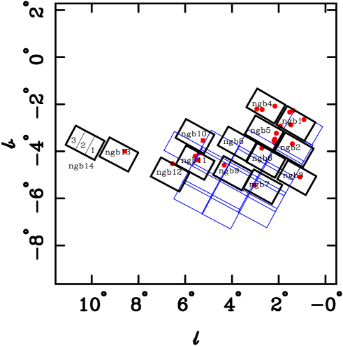
Figure 3: Locations of the 14 MOA Galactic Bulge fields and positions of transient events detected in 2000 shown in Galactic coordinates. Candidate microlensing events detected during 2000 are shown by the dots and the nova-like events are shown by the squares. The relative positions of the three CCDs are shown for field ngb14. The MOA fields observed during 1998–99 are also shown.

A number of interesting transient events were detected in real time during the 2000 Galactic Bulge observation season. These are listed in Table 1. Their positions are plotted in Galactic coordinates together with the MOA Bulge fields in Fig. 3. The majority of the events listed are probably microlensing events, but the list also includes some nova-like events. Nine of the events listed in Table 1 were issued as transient alerts.

The online analysis described in the previous sub-section involved a trade-off between analytical rigour and computing time. A detailed follow-up analysis was carried out on the events listed in Table 1. For a given event, 400$\times$400 pixel subframes were extracted from all flat-fielded observation images in the sequences. An astrometric reference was again selected from amongst the best quality sub-frames and the geometric alignment was repeated. Since we were now dealing with small images, we formed the subtraction reference by combining a selection of the very best seeing images. We required that the geometric alignment images selected in forming the reference involved small offsets from the astrometric reference less than 5 pixels. This ensured any pixel defects are localised to small regions on the combined image after geometrically aligning the individual images. Furthermore, as with the online analysis, we imposed the strict requirement that all stamps on the reference image used to solve for the kernel, be completely free of pixel defects. The image subtraction process was again carried out on all subframes. The use of small subframes made it easier to model spatial variations in the kernel and the differential background using smooth functions.

On a given observation image, the profile on a subtracted image at the position of a variable star follows the point-spread function on the corresponding unsubtracted image. In the follow-up analysis the integrated flux over these profiles was measured using empirical PSF models. For each event, a high signal to noise PSF was constructed from the reference image by combining small sub-frames centred on a number of bright, isolated, and non-saturated stars near the event position. For each observation image, this reference PSF was convolved with the corresponding kernel model derived for this image and evaluated at the event position to obtain a normalized empirical PSF profile for the given event on the given observation image. This PSF was then rescaled to fit the observed flux profile on the subtracted image to provide a measurement of the flux difference. The associated errors were determined in a self-consistent manner by applying the same measurement technique at the positions of constant stars in the field (which have flux differences of zero). The scatter in the flux difference measurements for these stars determined the frame-to-frame errors.

3.4 Interpretation of Difference Imaging Photometry

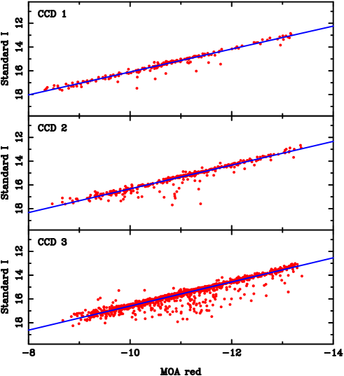
Figure 4: Calibration of MOA custom red passband measurements to the standard I band magnitude scale for the three CCDs of the camera MOA-cam2.

Difference imaging measures flux differences. This is a relatively unusual concept in astronomical photometry. To convert “delta flux” ($\Delta F$) measurements onto a magnitude scale, it is necessary to determine a corresponding “total flux”. This is given by

$$F=F_{\rm ref}+\Delta F$$ (6)

where $F_{\rm ref}$ is the flux of the object on the subtraction reference image. The reference flux may be measured by applying a profile fitting program such as Dophot to the reference image. Alternatively, one can derive the reference flux by fitting a theoretical profile, such as a microlensing profile, to the observed delta-flux light curve.

There are some situations where it may not be possible to measure the reference flux, and hence the total flux, for a particular event. For example, the event may be strongly blended with a close bright star making a reference flux measurement impossible. In such a situation, classical profile fitting photometry will not be able to yield a reliable light curve but difference imaging photometry will at least yield a delta flux light curve with each measurement unaffected by blending.

To obtain information in standard passbands, we used UBVI measurements of selected stars in Baade’s Window provided by OGLE [1999] that are contained in some of the MOA Bulge fields. The Dophot procedure was applied to the corresponding MOA reference images and the resulting star positions were cross-referenced with those of stars with UBVI measurements. As seen in Fig. 4 we find that measurements taken in the non-standard MOA red passband correlate well with measurements taken in the standard I passband. If the total flux of a particular measurement obtained by image subtraction photometry is known, a corresponding standard I measurement can be determined by the following relations for the three CCDs of MOA-cam2

$$I=\left\{\begin{array}[]{ll}25.8016+0.9704m_{\rm red}&\mbox{for CCD 1}\\ 26.2964+0.9970m_{\rm red}&\mbox{for CCD 2}\\ 26.9550+1.0316m_{\rm red}&\mbox{for CCD 3}\end{array}\right.$$ (7)

where $m_{\rm red}=-2.5\log(F)$ is the instrumental MOA red magnitude associated with the total flux measurement.

4 Events Detected During 2000

4.1 Microlensing Events

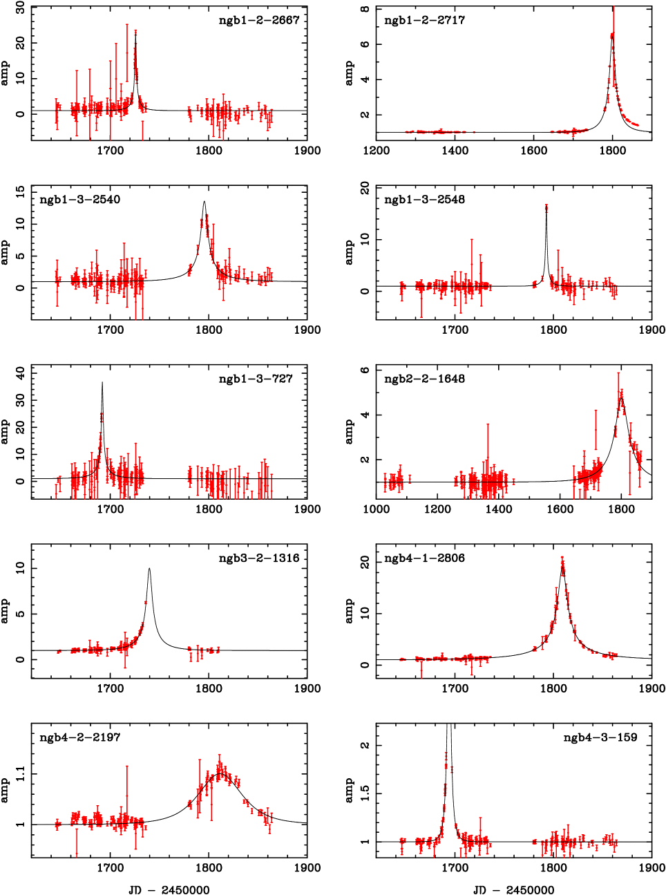
Figure 5: Candidate microlensing events detected in MOA Galactic Bulge fields ngb1, ngb2, ngb3, and ngb4 during 2000.

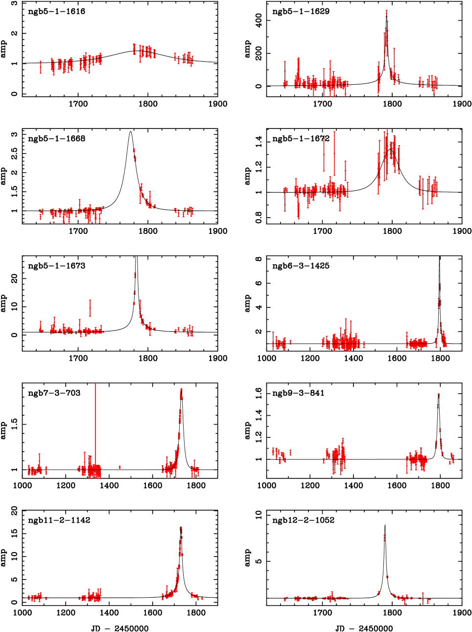
Figure 6: Candidate microlensing events detected in MOA Galactic Bulge fields ngb5, ngb6, ngb7, ngb9, ngb11, and ngb12 during 2000.

Figure 7: Contour plot of $\chi^{2}$ based on fitting a theoretical microlensing profile in ($A_{\rm max}$, $t_{\rm E}$) parameter space for event ngb6–3–1425. The contours correspond to confidence levels of 68%, 95%, and 99.73%.

Figure 8: Contour plot as in Fig. 7 for event ngb5–1–1629.

The observed flux difference for a microlensing event is given by

$$\Delta F=F_{\rm base}A\left(u(t)\right)-F_{\rm ref}$$ (8)

where $F_{\rm base}$ is the baseline flux and $F_{\rm ref}$ is the flux on the subtraction reference image. In general the reference image contains some lensed flux and is not equal to the baseline flux. Even if the source is not visible at baseline, the best seeing images used to form the subtraction reference image may occur when the source is lensed. This is true for some of the microlensing events presented here.

If the reference image was formed by combining $N_{\rm ref}$ images taken at times $\{t_{i}\}$, the reference flux for a microlensing event is given by

$$F_{\rm ref}=\frac{F_{\rm base}}{N_{\rm ref}}\sum_{i}A(u(t_{i}))$$ (9)

The amplification, $A(u)$, expressed in terms of the distance, $u$, of the lens star from the line-of-sight to the source star expressed in units of the Einstein radius is given by [1986]

$$A(u)=\frac{u^{2}+2}{u\sqrt{u^{2}+4}}$$ (10)

where

$$u(t)=\sqrt{u_{\rm min}^{2}+\left(\frac{t-t_{\rm max}}{t_{\rm E}}\right)^{2}}.$$ (11)

Here $u_{\rm min}$ is the minimum value of $u$ during an event, $t_{\rm E}$ is the characteristic Einstein radius crossing timescale, and $t_{\rm max}$ is the time of maximum amplification. The time $t_{\rm E}$ is equal to $r_{\rm E}/v_{\rm T}$ where $v_{\rm T}$ is the transverse velocity of the lens with respect to the line-of-sight to the source.

Table 2: Fitted Parameters of Microlensing Candidates

MOA ID			$A_{\rm max}$			$t_{\rm E}$ / days			$t_{\rm max}$	I magnitude
Field	CCD	ID	lower	best	upper	lower	best	upper	JD$-$2450000	baseline
ngb1	2	2667	10.7	22.8	-	8.0	14.8	-	1725.74	19.96
ngb1	2	2717	5.8	6.5	7.0	40.2	43.0	46.1	1799.62	14.16
ngb1	3	727	12.8	36.8	-	11.0	29.1	-	1691.98	20.20
ngb1	3	2540	5.9	13.6	60.8	24.2	40.7	140.8	1795.54	19.24
ngb1	3	2548	5.0	16.5	118.4	5.0	9.5	40.0	1792.80	19.32
ngb2	2	1648	3.5	4.8	6.6	79.2	95.7	118.4	1801.13	17.74
ngb3	2	1316	3.2	10.0	-	11.2	26.7	-	1739.76	18.03
ngb4	1	2806	15.7	19.0	24.3	69.4	83.0	104.6	1809.15	17.49
ngb4	2	2197	1.0	1.1	3.3	14.0	19.8	64.0	1812.50	14.11
ngb4	3	159	2.0	3.7	-	3.9	5.1	6.5	1693.98	15.80
ngb5	1	1616	1.3	1.4	-	39.0	57.2	-	1785.17	15.12
ngb5	1	1629	68.2	434.8	-	84.0	507.0	-	1791.86	22.74
ngb5	1	1668	1.4	3.1	15.0	12.0	20.3	60.0	1775.17	15.74
ngb5	1	1672	1.1	1.3	4.3	9.0	16.6	44.0	1796.93	15.38
ngb5	1	1673	27.8	49.1	-	29.6	42.3	72.0	1783.65	18.11
ngb6	3	1425	6.3	8.7	12.4	12.0	14.5	17.6	1796.00	17.42
ngb7	3	703	1.6	1.9	2.2	13.1	15.2	17.1	1732.87	15.03
ngb9	3	841	1.2	1.6	5.0	6.0	8.8	20.0	1791.89	14.71
ngb11	2	1142	13.9	16.5	20.2	63.1	74.4	90.1	1730.31	17.65
ngb12	2	1052	6.3	9.0	31.1	8.8	10.9	14.6	1789.68	16.80

We fitted the theoretical single lens light curve given by Eqns 8–11 to the data for candidate microlensing events using four parameters $F_{\rm base}$, $u_{\rm min}$, $t_{\rm E}$, and $t_{\rm max}$. The light curves are shown in Figs. 5–6 where the $\Delta F$ data points have been converted to amplifications using the fitted parameters. We note that for some of the events, the baseline flux is below the observational threshold. However, we could still derive a best fit value for $F_{\rm base}$. This is essentially an extrapolation of the light curve from where the event is visible down to the baseline level. In these events this value for $F_{\rm base}$ is used to calculate amplifications in plotting the light curves in Figs. 5–6. We address the issue of measuring microlensing parameters for these types of events in detail below.

The microlensing parameters $t_{\rm E}$ and the peak amplification $A_{\rm max}$ (calculated directly from $u_{\rm min}$ using Eqn. 10) are the interesting physical quantities in a microlensing event. Both quantities can be measured for microlensing events with good sampling from the baseline to the peak. However, for high magnification events sampled only around the times of peak amplification, it is possible only to measure the quantity $t_{\rm eff}=t_{\rm E}u_{\rm min}$ which is degenerate in the two parameters of interest [1996]. We investigated the extent to which these parameters can be constrained by mapping $\chi^{2}$ in the two dimensional parameter space corresponding to $A_{\rm max}$ and $t_{\rm E}$. For each light curve, we fitted Eqns 8–11 for a sample of fixed $(A_{\rm max},t_{\rm E})$ pairs with the remaining parameters, $F_{\rm base}$ and $t_{\rm max}$, allowed to float.

In Fig. 7 we show a contour map of $\chi^{2}$ in $(A_{\rm max},t_{\rm E})$ space for the event ngb6–3–1425. The contours connect equal values of $\chi^{2}_{\rm min}+\Delta\chi^{2}$ for $\Delta\chi^{2}=(2.3,6.2,11.8)$. These formally correspond to confidence limits of 68%, 95%, and 99.73% respectively for the simultaneous estimation of two interesting parameters [1976]. Event ngb6–3–1425 can be described as a “classical” microlensing event where the source was resolved and visible at baseline and the light curve was well sampled both at its baseline and during its lensing phase. In this case both $A_{\rm max}$ and $t_{\rm E}$ are well constrained.

In contrast the parameter space of the event ngb5–1–1629 was not as well constrained as can be seen in Fig. 8. A close inspection of the baseline images for this event did not show any visible object at the position of the source while it was clearly visible during amplification. This event is clearly characteristic of one which is amplified from below the observational threshold to above the threshold. Such events are only observable around the times of high magnification, and only lower limits can be inferred for $A_{\rm max}$ and $t_{\rm E}$. It is nevertheless noteworthy that one can infer that this event had a peak amplification well in excess of 70.

Alcock et al. [2000] proposed classifying microlensing events found by DIA as either classical or “pixel lensing” events following the definition by Gould [1996] of pixel lensing events as microlensing of unresolved sources. A source may be unresolved if it is strongly blended with nearby stars or if it is too faint to be observed at baseline. Since DIA is unaffected by blending we suggest here a classification based just on amplification. Events would then fall into two types: those amplified from below the observation threshold and those amplified from above. For those events whose baselines are below the detection and hence measurement threshold, it is only possible to obtain lower limits on $A_{\rm max}$ and $t_{\rm E}$. We suggest that in DIA it is important to be able to distinguish between the two types of events as this affects the extent to which the microlensing parameters can be constrained.

In Table 2 we summarize the results of this analysis for all 20 microlensing events showing best fit values for $A_{\rm max}$ and $t_{\rm E}$ along with 95% lower and upper limits where possible. The fitted baselines fluxes were converted to I magnitudes using the calibration information described in Section 3.4. The parameters of one event, ngb3–2–1316, are poorly constrained as this event did not receive adequate temporal coverage.

Of the 20 events listed in Table 2, half of them have best fit peak amplifications around 10 or more, and six have lower limits of $A_{\rm max}$ greater than 10. This is a large fraction of high magnification events when compared with the corresponding fractions from the MACHO and OGLE surveys. Since these groups use profile fitting photometry in their on-line analysis, their measurements are in general affected by blending and therefore the derived values of $A_{\rm max}$ tend to be underestimated. More importantly, DIA is sensitive to microlensing events whose source stars are too faint to be detected at baseline.

The large fraction of detected events with high magnification has useful implications for studies of extra-solar planets, low mass stars and stellar atmospheres, as noted in the introduction.

4.2 MOA–2000–BLG–11: A Microlensing Parallax Event

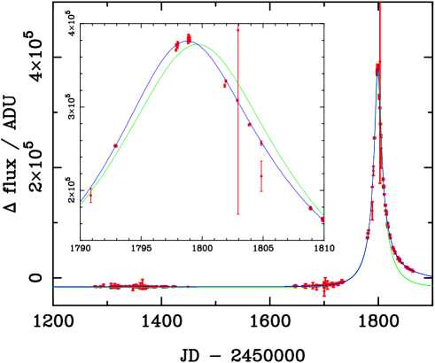
Figure 9: Delta-flux light curve of MOA–2000–BLG–11 with standard and parallax microlensing fits.

Table 3: MOA-2000–BLG–11: Standard and parallax microlensing fit parameters

Parameter	Standard	Parallax
$I_{\rm base}$	14.16	14.78
$t_{0}$	JD2451799.62	JD2451837.62
$t_{\rm E}$	43.04 days	69.69 days
$u_{\rm min}$	0.157	0.224
$\tilde{v}$	-	42.52 km s-1
$\theta$	-	$-$76$\aas@@fstack{\circ}$20
$\chi^{2}$/dof	18027.6/401	1071.6/399

The light curve of event ngb1–2–2717, which was alerted as MOA–2000–BLG–11, is not well described by the standard microlensing profile given by Eqns. 7–8. The light curve exhibits an asymmetric profile which is characteristic of parallax microlensing. Here, a distortion arises from the circularly accelerating motion of the Earth around the Sun. When including this motion, the distance between the lens star and the source star (given by Eqn. 8 for the constant velocity case) contains two extra parameters: the angle, $\theta$, between the transverse motion of the lens and the transverse speed, $\tilde{v}$, projected onto the solar position. The full mathematical details can be found in Alcock et al. [1995], Mao [1999], and Dominik [1998].

The light curve of MOA–2000–BLG–11 is shown in Fig. 9 along with the best fit standard constant velocity and parallax microlensing models. The derived parameters are given in Table 3. At 75.1 days, the duration of MOA-2000–BLG–11 is rather short compared with the durations for previously detected parallax events of 111.3 days for the first parallax event found by the MACHO group [1995], 118.1 days for OGLE–99–CAR–1 [1999], and 156.4 days for OGLE–00–BUL–43 [2001].

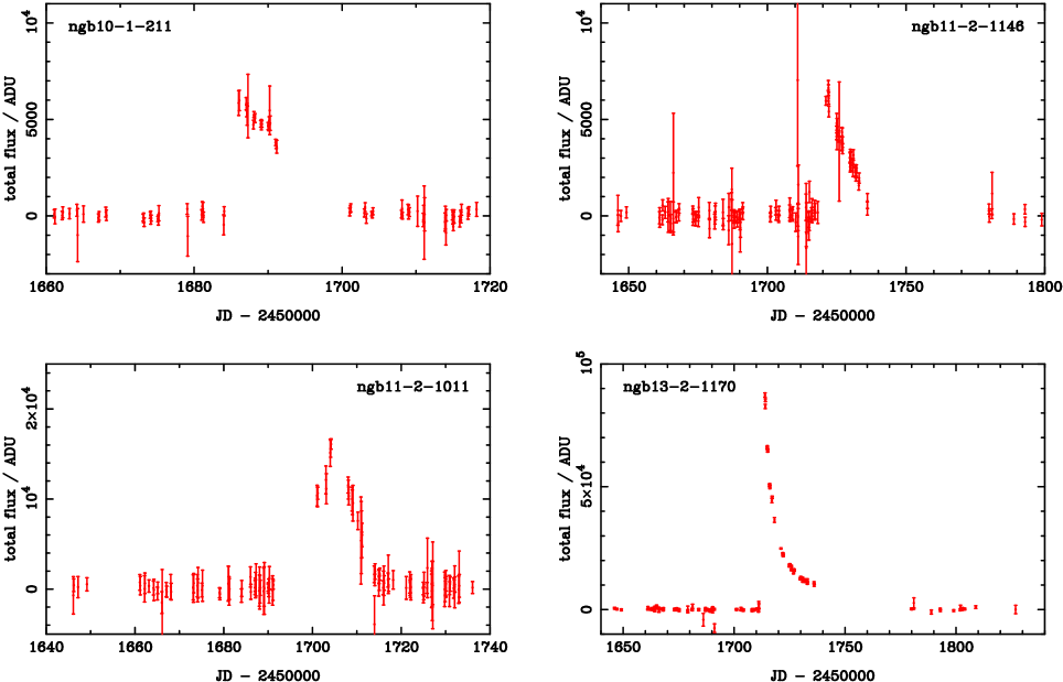
Figure 10: Light curves of nova-like events detected during 2000.

Measurements of microlensing parallax events partially resolve the degeneracy in the mass, lens distance, and transverse velocity contained in the standard microlensing equation. Assuming negligible velocity dispersion in the disk and the bulge, the transverse speed projected onto the solar position can be written as

$$\tilde{v}=\frac{220x}{1-x}{\rm kms}^{-1}$$ (12)

where $x=D_{l}/D_{s}$ with $D_{l}$ being the distance to the lens and $D_{s}$ the distance to the source star. Following Alcock et al. [1995] the mass of the lens, $M_{l}$, can written as

$$M_{l}=\frac{1-x}{x}\frac{\tilde{v}^{2}t_{\rm E}^{2}c^{2}}{4GD_{s}}.$$ (13)

Substituting the parameters obtained from our parallax fit and assuming $D_{s}=8$ kpc we obtain $D_{l}\sim 1.4$ kpc and $M_{l}\sim 0.3M_{\sun}$ for the lens star. It would then contribute very little light through the course of the event. It should be noted that, provided the lens star is constant, the contribution of any flux from the lens star is canceled out in delta-flux measurements.

4.3 Nova-like Events

Table 4: Summary of the characteristics of nova-like events detected in 2000. The column, $\Delta I$, denotes the change in I magnitude during the rise of the event from its quiescent state to its high state.

MOA ID			peak I	$\Delta I$	$t_{1/2}$
Field	CD	ID			days
ngb10	1	211	16.64	$>$2.4	5
ngb11	2	1011	15.78	$>$3.3	3
ngb11	2	1146	16.75	$>$2.3	7
ngb13	2	1211	13.95	$>$5	4

Some events with light curves showing nova-like profiles were found. We present them in Fig. 10 and Table 4 to illustrate the potential for detecting new types of objects. None of the events was visible in the MOA images during their times of minimum light. Event ngb13–2–1170 (alerted as MOA–2000–BLG–6) is clearly characteristic of a dwarf nova. This event rose by more than five magnitudes in less than three days peaking at $I=13.95$. Event ngb11–2–1146 also appears to be the tip of a dwarf nova decay just above the detection limit. Event ngb10–1–211 is also nova-like but the decay is not as smooth as the other events. At the position of event ngb11–2–1011, the MACHO database contains an object whose corresponding light curve undergoes flaring episodes about once per year (D. Bennett, private communication).

4.4 Asteroids

As well as measurements on variable stars, difference imaging analysis can be employed to study moving objects. In Fig. 11 we show subimages of three exposures of MOA field ngb1 on CCD number 1 taking during one night. The subimages include the original unsubtracted images along with their corresponding subtracted images. The exposures were taken over a time interval of approximately 1.6 hours. An object moving across the field of view can clearly be seen. The positions and magnitudes of this object measured on each image are listed in Table 5. A crosscheck with Guide 7.0 revealed asteroid (3680) Sasha at these positions and times.

The associated transverse velocity across the sky for this object is $19.2\arcsec$ hour^-1. Frequent sampling of the fields are required if one is to track the motion of such fast moving objects during a night. Sampling the fields once per night would merely result in spike events at asteroid positions. The MOA data base now contains subtracted images derived from a large number of nights where the sampling rate was three or more times per night. We are currently exploring ways of exploiting this data base to study asteroids.

Table 5: Astrometry and Photometry of Asteroid

	Coordinates (J2000.0)
JD-2450000	RA	DEC	I magnitude
1675.066760	17:56:23.33	$-$29:54:51.4	15.33
1675.133438	17:56:21.28	$-$29:55:06.5	15.19
1675.197859	17:56:19.28	$-$29:55:21.0	15.28

5 Summary

It has been demonstrated that real-time difference imaging of an extensive database is possible. The procedure employed by MOA is a database management system rather than a linear reduction pipeline. A variety of levels of automation are possible but the final selection of events is by human intervention.

To minimize hardware constraints, two reduction procedures were developed, one for online analysis of large numbers of large images, and one for follow-up, accurate analyses of selected events. As our on-site computing power expands, we plan to transfer elements of our follow-up procedure to the online analysis. We also plan to increase the conversion rate of internally monitored candidate events to actual alerts issued to the microlensing community.

We have demonstrated that a high fraction of events detected by difference imaging have high magnification. This should have useful implications for studies of extra-solar planets and faint stars provided the peaks of future events are monitored photometrically and/or spectroscopically by the microlensing and other astronomical communities.

Our observational strategy has been to monitor a moderate area of the Galactic Bulge, $17\deg^{2}$, fairly frequently, i.e. up to six times per night. This is a compromise between survey area and sampling rate that we plan to continue. It has enabled the detection of some unusual types of events, including nova-like transients and an asteroid, as well as microlensing events of high magnification.

References

- [1997] Abe, F., et al., 1997, in “Variable Stars and the Astrophysical Returns of Microlensing Surveys”, eds. R.Ferlet, J. Maillard, and B. Raban, Editions Frontieres, France, p. 75.
- [2000] Albrow, M.D., et al., 2000, ApJ, 535, 176
- [2001] Alard, C., 2001, MNRAS, 320, 341
- [1999] Alard, C., 1999, A&A, 342, 10
- [1998] Alard, C., Lupton, R.H., 1998, ApJ, 500, 37
- [1993] Alcock, C. et al., 1993, Nature, 365, 621
- [1995] Alcock, C. et al., 1995, ApJ, 454, L125
- [1999a] Alcock, C. et al., 1999a, ApJ, 521, 602
- [1999b] Alcock, C. et al., 1999b, ApJS, 124, 171
- [2000] Alcock, C. et al., 2000, ApJ, 541, 734
- [1993] Aubourg, E., et al., 1993, Nature, 365, 623
- [1976] Avni, Y., 1976, ApJ, 210, 642
- [2001] Bond, I.A., et al., 2001, submitted to MNRAS
- [1998] Dominik, M., 1998, A&A, 329, 361
- [1996] Gould, A., 1996, ApJ, 470, 201
- [1997] Griest K.G., Safizadeh, N., 1997, ApJ, 480, 196
- [1998] Han, C., 1998, ApJ, 500, 569
- [2001] Kane, S.R., Sahu, K.C., 2001, astro-ph/0101092
- [1996] Lennon, D., Mao, S., Fuhrmann, K., Thomas, G., 1996, ApJ, 471, L23
- [1997] Lennon, D., et al., 1997, The Messenger, 90, 30
- [1999] Mao, S., A&A, 350, L19
- [1998] Minniti, D., et al., 1998, ApJ, 499, L175
- [1986] Paczyński, B., 1986, ApJ, 304, 1
- [1999] Paczyński, B. et al., 1999, Acta Astron., 49, 319
- [1995] Phillips, A.C., Davis, L.E., 1995, ASP conf. series, 77, Astronomical Data Analysis and Software Systems IV, ed. R.A. Shaw et al., 297
- [2000] Rhie, S., et al., 2000, ApJ, 533, 378
- [1993] Schecter, P., Mateo, M., Saha, A., 1993, PASP, 105, 1342
- [2001] Sozyński, I. et al., 2001, astro-ph/0012144
- [1996] Tomaney, A.C., Crotts, A.P., 1996, AJ, 112, 2872
- [1992] Udalski, A., Szymański, M., Kaluźny, J., Mateo, M., 1992, Acta Astron., 42, 253
- [2000] Woźniak, P.R., 2000, astro-ph/0002510
- [2000] Yanagisawa, T. et al., 2000, Exp. Astron., 10, 519