THE NACRE THERMONUCLEAR REACTION COMPILATION
AND BIG BANG NUCLEOSYNTHESIS

Abstract

The theoretical predictions of big bang nucleosynthesis (BBN) are dominated by uncertainties in the input nuclear reaction cross sections. In this paper, we examine the impact on BBN of the recent compilation of nuclear data and thermonuclear reactions rates by the NACRE collaboration. We confirm that the adopted rates do not make large overall changes in central values of predictions, but do affect the magnitude of the uncertainties in these predictions. Therefore, we then examine in detail the uncertainties in the individual reaction rates considered by NACRE. When the error estimates by NACRE are treated as $1\sigma$ limits, the resulting BBN error budget is similar to those of previous tabulations. We propose two new procedures for deriving reaction rate uncertainties from the nuclear data: one which sets lower limits to the error, and one which we believe is a reasonable description of the present error budget. We propagate these uncertainty estimates through the BBN code, and find that when the nuclear data errors are described most accurately, the resulting light element uncertainties are notably smaller than in some previous tabulations, but larger than others. Using these results, we derive limits on the cosmic baryon-to-photon ratio $\eta$, and compare this to independent limits on $\eta$ from recent balloon-borne measurements of the cosmic microwave background radiation (CMB). We discuss means to improve the BBN results via key nuclear reaction measurements and light element observations.

1 Introduction

Big bang nucleosynthesis (BBN) has long played a key role in the standard cosmology. The concordance between the predicted and observed light element abundances (Walker et al. 1991; Olive, Steigman, & Walker 2000) gives confidence that the basic framework is working down to epochs of $t\sim 1$ sec, and $z\sim 10^{10}$. The theory-observation comparison also probes particle physics in the early universe (Sarkar 1996; Olive & Thomas 1999; Lisi, Sarkar, & Villante 1999), and quantifies the allowed range in the baryon-to-photon ratio $\eta=n_{\rm B}/n_{\gamma}$ (Fields & Olive 1996, Fields et al. 1996, Schramm & Turner 1998) and thus the cosmic baryon density parameter $\Omega_{\rm B}h^{2}$ (where $\Omega_{i}=\rho_{i}/\rho_{\rm crit}=8\pi G\rho_{i}/3H_{0}^{2}$, and $H_{0}=100h\ {\rm km\ s^{-1}\ Mpc^{-1}}$).

Over the past decade, a major thrust of research in BBN has been towards increasing the rigor of the analysis. On the theory side, the key innovation was to calculate the errors in the light element predictions in a systematic and statistically careful way. This was done using Monte Carlo analyses (Krauss & Romanelli 1990; Smith, Kawano, & Malaney 1993; Kernan & Krauss 1995; Hata et al. 1995; Fiorentini et al. 1998; Nollett & Burles 2000), which account for nuclear reaction uncertainties and their propagation into uncertainties in the light element abundance predictions. These calculations are essential because they allow for a careful statistical comparison of BBN theory with observational constraints; in addition, they point the way toward improvements in the theory calculation. Just as BBN theoretical and observational ingredients have been sharpened, so have the tools for comparing the two. Statistical tests involving likelihood analyses (Hata et al. 1995; Fields, Kainulainen, Olive, & Thomas 1996; Lisi, Sarkar, & Villante 1999) have been developed and performed.

A focus on rigor in BBN will soon be rewarded, as cosmology moves toward a precision era. Specifically, the observations of the anisotropies in the cosmic microwave background (CMB) will allow for very precise determination of cosmological parameters, including $\Omega_{\rm B}h^{2}$ (or, equivalently, $\eta$). A comparison of $\eta$ as determined by BBN and the CMB will provide a fundamental test of cosmology. In addition, as pointed out by Schramm & Turner (1998) and as shown in detail below, increasingly accurate CMB data can ultimately transform BBN into a much sharper probe of the early universe and of chemical evolution.

Along with the neutron lifetime, eleven key nuclear reaction rates represent the dominant sources of error the BBN calculation (Smith, Kawano, & Malaney skm (1993), hereafter SKM; and §4 below). Thus, the choice of thermonuclear reaction rates, and their uncertainties, will determine the accuracy of the final predictions. Most recent work on BBN has used the Caughlan & Fowler cf (1988) compilation, with updates due to SKM and others. The SKM error budget has been the standard for all of the subsequent Monte Carlo work except for that of Nollett & Burles nb (2000), who create their own rates from the nuclear data, but do not present the thermonuclear rates by themselves. The recent work by NACRE (Angulo et al. nacre (1999)) represents a significant new effort to critically evaluate nuclear cross section data and derive thermonuclear rates. Moreover, the NACRE compilation includes estimates of uncertainties in the reaction rates.

We therefore have examined the impact of the NACRE rates on BBN. This issue has also been studied by Vangioni-Flam, Coc, & Cassé vcc (2000). These authors considered the impact of the error range estimated by NACRE by calculating the effect of individual rates on the primordial abundances. Vangioni-Flam, Coc, & Cassé vcc (2000) then estimated the effect of the ensemble of rates by placing all rates at their maximum and minimum variation. Here, we will extend this work in several ways. We will use a full Monte-Carlo treatment, which allows for a quantitative statement about the propagation of the errors. In addition, we examine the impact of different error assignments: (1) those of the NACRE group themselves, which give useful estimates of the range of uncertainty but are not defined in a uniform manner; as well as (2) the results of our own error analyses, which we derive from the nuclear data according to simple but uniform procedures.

This paper is organized as follows. We will describe the NACRE recommended rate uncertainties in §2. In §3 we compare the NACRE uncertainty estimations with other estimates based on the nuclear reaction data. These different error estimates are used to predict light element uncertainties via Monte Carlo BBN calculations (§4). The results are compared with observations via likelihood analyses in §5, and discussed in terms of the predictions for $\eta$. We discuss the agreement of our predictions with current CMB data in §6, and anticipate the impact of high-quality data which will arise from future CMB space-based experiments. Our conclusions are summarized in §7.

2 The NACRE Compilation

In an effort to update the thermonuclear reaction rate compilation by Caughlan & Fowler (1988), the NACRE collaboration has presented a detailed analysis of 86 charge induced nuclear reactions. Out of these reactions we will discuss the 7 reactions NACRE has in common with the 11 reactions from SKMskm (1993), whose errors dominate the uncertainties in the abundances.(see §2.3)

2.1 Reaction Rate Formalism

The nuclear reaction inputs to BBN take the form of thermal rates. These rates are computed by averaging nuclear reaction cross sections over a Maxwell-Boltzmann distribution of energies. The thermonuclear reaction rate at some temperature $T$, is given by the following integral:

$$N_{A}\langle\sigma v\rangle=N_{A}\left(\frac{8}{\pi\mu(k_{B}T)^{3}}\right)^{\frac{1}{2}}\int_{0}^{\infty}\sigma(E)E\exp\left(-\frac{E}{k_{B}T}\right)dE$$ (1)

where $N_{A}$ is Avogadro’s number, $v$ the relative velocity, $\mu$ gives the reduced mass of the nuclei, $k_{B}$ Boltzmann’s constant and $\sigma(E)$ yields the cross section at center of mass energy $E$.

The charge induced cross sections can be decomposed into

$$\sigma(E)=\frac{S(E)\exp\left(-2\pi\zeta\right)}{E},$$ (2)

where $S(E)$ gives the astrophysical $S$-factor, $\zeta$ is the Sommerfeld parameter, defined by

$$\zeta=Z_{1}Z_{2}\left(\frac{e^{2}}{\hbar c}\right)\left(\frac{c}{v}\right)=Z_{1}Z_{2}\left(\frac{e^{2}}{\hbar c}\right)\left(\frac{\mu c^{2}}{2E}\right)^{\frac{1}{2}}.$$ (3)

Here the $Z_{i}$’s are the charges of the nuclei in units of the proton charge $e$.

For neutron induced reactions, the cross section can be written as follows:

$$\sigma(E)=\frac{R(E)}{v},$$ (4)

where $R(E)$, the $R$-factor, can be a slowly varying function of energy, and is similar to an $S$-factor.

2.2 Recommended Thermonuclear Rates

Generally speaking, NACRE follows the standard path (outlined in the previous section) for going from nuclear data to thermonuclear rates. NACRE has compiled an extensive tabulation of nuclear reaction cross section data, which is available in a very convenient form online at the NACRE website http://pntpm.ulb.ac.be/nacre.htm. For each experiment, the NACRE collaboration has organized cross section data into useful tables, providing information on the measured cross sections and their total error as a function of energy. These tabulations are invaluable for the analysis of error propagation.

It is important to have a consistent method of analyzing cross sections and computing reaction rates. The data sets provided by NACRE over the relevant energy ranges for BBN have large variations in both quality and quantity. Thus, NACRE critically evaluates the experimental data and gives different data sets different weights in determining rates. The NACRE collaboration considers only charged induced reactions, thus leaving out several important reactions for BBN. Therefore we have to include the neutron-induced reactions and one deuteron-induced reaction by the SKM compilation. The reactions used from each are shown in Table 1. For completeness we will describe the approach for the neutron-induced reactions as well.

Once the cross section data (and errors) are gathered, they are put into $S$-factor or $R$-factor form. NACRE fits these factors to analytic functions. For non-resonant data, a polynomial of order 2 to 3, is used. Some data are fit from theory (e.g., NACRE uses Kajino’s kajino (1986) fits for $t(\alpha,\gamma)\mbox{${}^{7}{\rm Li}$}$ and $\mbox{${}^{3}{\rm He}$}(\alpha,\gamma)\mbox{${}^{7}{\rm Be}$}$), while for resonant data a Briet-Wigner or R-matrix fit is performed (e.g., for $t(d,n)\mbox{${}^{4}{\rm He}$}$). The fits are required to be a good representation of the data by a $\chi^{2}$ analysis, taking precedence over agreement with theory.

The evaluated cross section fits, $S_{\rm fit}(E)$ are used to determine thermal rates (via (1)) for a grid of temperatures, $T$, ranging from $T_{9}=.001-10$, where $T=T_{9}\times 10^{9}$K. These results are subsequently fit to a prescribed function of $T_{9}$. One should note that the NACRE fits do not reflect the analytic approximation for the thermal rates used by Caughlan & Fowler (1988). Namely, Caughlan & Fowler put non-resonant thermal rates in the form $(\sum_{j}c_{j}T_{9}^{j/3})\exp(a/T_{9}^{1/3})$. NACRE modifies this approach, keeping the same exponential dependence, but changes the prefactor from a polynomial in $T_{9}^{1/3}$ to one in $T_{9}$: $(\sum_{j}c^{\prime}_{j}T_{9}^{j})\exp(a^{\prime}/T_{9}^{1/3})$. The main reason for the form of their fit is to get fast convergence to the numerical data. In some cases (e.g. $\mbox{${}^{3}{\rm He}$}(d,n)\mbox{${}^{4}{\rm He}$}$ and $\mbox{${}^{7}{\rm Li}$}(p,\alpha)\mbox{${}^{4}{\rm He}$}$) additional factors are used to improve the fit to the numerical results.

Table 1: Key Nuclear Reactions for BBN

Source	Reactions
NACRE	$d(p,\gamma)\mbox{${}^{3}{\rm He}$}$
	$d(d,n)\mbox{${}^{3}{\rm He}$}$
	$d(d,p)t$
	$t(d,n)\mbox{${}^{4}{\rm He}$}$
	$t(\alpha,\gamma)\mbox{${}^{7}{\rm Li}$}$
	$\mbox{${}^{3}{\rm He}$}(\alpha,\gamma)\mbox{${}^{7}{\rm Be}$}$
	$\mbox{${}^{7}{\rm Li}$}(p,\alpha)\mbox{${}^{4}{\rm He}$}$
SKM	$p(n,\gamma)d$
	$\mbox{${}^{3}{\rm He}$}(d,p)\mbox{${}^{4}{\rm He}$}$
	$\mbox{${}^{7}{\rm Be}$}(n,p)\mbox{${}^{7}{\rm Li}$}$
This work	$\mbox{${}^{3}{\rm He}$}(n,p)t$
PDG	$\tau_{n}$

As noted above, some of the rates are not provided by NACRE. In these cases, the SKM rates as indicated in Table 1 are used. One of these, $\mbox{${}^{7}{\rm Be}$}(n,p)\mbox{${}^{7}{\rm Li}$}$, is a $n$-capture reaction for which a large amount of data is available. The deuteron-induced reaction ($\mbox{${}^{3}{\rm He}$}(d,p)\mbox{${}^{4}{\rm He}$}$), is fit as a charged particle reaction using the Caughlan & Fowler prescription, as discussed in the previous paragraph.

Several reactions deserve special mention. As noted by SKM and emphasized recently by Nollett & Burles nb (2000), the $p(n,\gamma)d$ reaction suffers from a lack of data in the BBN energy range. Also, $p(n,\gamma)d$ has only 4 data points (not available when SKM did their study) in the relevant energy range $\lesssim 1$ MeV. Fortunately, this reaction is well-described theoretically. Here we follow both SKM and Nollett & Burles, by adopting the theoretical cross sections of Hale et al. (1991), which provide an excellent fit to the four available data points by Suzuki suz95 (1995) and Nagai nagai (1997). Nevertheless, despite the present agreement between theory and data, the importance of this reaction–which controls the onset of nucleosynthesis–demands that the theoretical cross section fit be further tested by accurate experiment. We urge further investigation of this reaction.

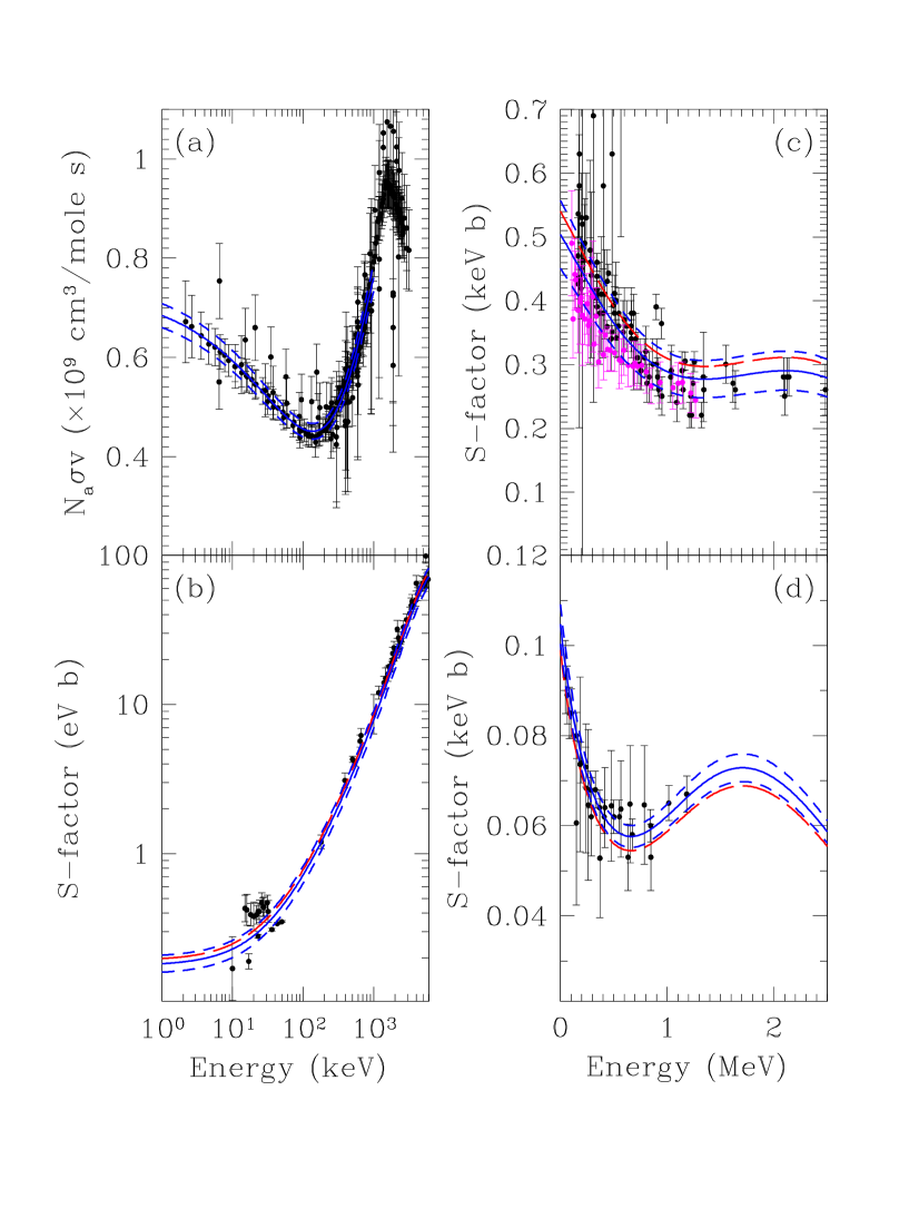
Figure 1: Experimental data and $R$- and $S$-factor fits for four key reactions. The solid curves are our renormalized fits, with our sample variance error bands given by the short dashed curves. For the $S$-factor curves, data are given in NACRE, whose raw fits are given by the long dashed curves. a) The $R$-factor for $\mbox{${}^{3}{\rm He}$}(n,p)t$. The data are those of SKM with the addition of Brune et al. brune99 (1999). The fit is ours, as described in §2.2. b) The $S$-factor data for $d(p,\gamma)\mbox{${}^{3}{\rm He}$}$. c) The $S$-factor data for $\mbox{${}^{3}{\rm He}$}(\alpha,\gamma)\mbox{${}^{7}{\rm Be}$}$. d) The $S$-factor data for $t(\alpha,\gamma)\mbox{${}^{7}{\rm Li}$}$.

Since SKM, Brune et al. brune99 (1999) have added new and very precise data for $\mbox{${}^{3}{\rm He}$}(n,p)t$ (see Figure 1a). This has greatly reduced the uncertainty in this reaction. In order to use these data, we have refit the $R$ factor in the manner of SKM and Brune et al., using a third order polynomial in $v$ and the entire world data set. We arrive at fit parameters very similar to those of SKM and Brune et al., with $N_{A}\langle\sigma v\rangle=7.3546\times 10^{8}(1-0.7757T_{9}^{1/2}+0.5376T_{9}-0.1018T_{9}^{3/2})\ {\rm cm^{3}\ s^{-1}\ g^{-1}}$.

The weak reactions which govern $n\leftrightarrow p$ interconversion also deserve mention. These reactions are a strong function of temperature, but the rates can be scaled to a single laboratory measurement, the neutron lifetime $\tau_{n}$. Thus, the uncertainty in the weak rates is set by the uncertainty in $\tau_{n}$. Here, we have adopted the value recommended by the Particle Data Group, $\tau_{n}=885.7\pm 0.8$ s. This value reflects the recent and very precise measurement of Arzumanov et al. arz (2000), and has considerably reduced the errors of the Particle Data Group world average from the old determination of $886.7\pm 1.9$ s (Groom et al. PDG (2000)).

It is also important to include the small but non-negligible corrections to the tree-level weak rates. These include a number of contributions, such as radiative corrections (Dicus et al. dicus (1982); Heckler heckler (1994); Esposito, Mangano, Miele, & Pisanti 2000a ), nonequilibrium neutrino heating during $e^{\pm}$ annihilation (Dodelson & Turner dt (1992)), and finite nucleon mass and finite temperature effects (e.g., Seckel seckel (1993); Kernan ker (1993); Lopez & Turner lt (1999); Esposito, Mangano, Miele, & Pisanti 2000a ). These corrections have been implemented in our code as has been described in detail in Olive, Steigman, & Walker osw00 (2000). As discussed there, the differences in the ${}^{4}{\rm He}$ yields between our code and that of Lopez & Turner lt (1999) are $0.0001\pm 0.0001$ for $1\leq\eta_{10}\leq 10$.

2.3 Uncertainty Limits

NACRE uses data uncertainties in two ways, for the evaluation of mean rates and the evaluation of errors. For the mean (“adopted”) rates, they use the data errors to weight sets via a $\chi^{2}$ analysis. They also use the data errors to estimate the uncertainty range for these “adopted” rates. This is not done in a strict statistical way, and thus is not presented as, e.g., “1$\sigma$” error, but rather as “high” and “low” limits to the thermal rates.

The “high” and “low” limits are derived in different ways for different reactions. In the case where there happens to be two discrepant data sets, NACRE performs a $\chi^{2}$ analysis for each of the two data sets, adopting the set with the larger $S$-factor as their “high” limit, and the set with smaller $S$-factor as their “low” limit. The “adopted” value for their mean is simply the unweighted average of the “high” and “low” limits (e.g., $d(p,\gamma)\mbox{${}^{3}{\rm He}$}$).

3 A Comparison of Nuclear Reaction Uncertainty Estimations

The power of BBN theory to test and constrain cosmology and particle physics derives from the ability to calculate accurately the mean values and uncertainties in light element abundances as a function of $\eta$. The Monte Carlo analyses of BBN which provide these results are in turn only as good as the input nuclear and weak error budget. It is thus crucial to make the most accurate estimates possible, in a way that is appropriate for the cross section data sets and the thermal rate compilation one uses.

Given the importance of the error propagation, we will explore different methods of doing this for the NACRE compilation. We first examine NACRE’s own, “high/low” limits. As these are not uniformly derived, we also consider two other error budgets, which illustrate issues in error propagation and subsequent impact on BBN. In this section, we will describe the error propagation methods, and our implementation of them. We will then examine the BBN results using these errors in the following section (§4).

3.1 Tailoring Rates and Uncertainties for BBN

Since the error analysis of the rates by NACRE is not done in a strict statistical way, it becomes important to develop a general, statistically sound method for determining an accurate mean and error for the application to BBN. To do this, we will compare the NACRE theoretical $S$-factor fits to the data sets they use. For the theoretical fits $S_{\rm fit}(E)$, we for the most part use the analytical forms published in the NACRE paper. When these were unpublished, NACRE kindly made available their fits (or in the case of $t(d,n)\mbox{${}^{4}{\rm He}$}$, a tabular form). These fits are valid for different energy ranges depending on the reaction, but in all cases cover an energy band which includes and extends beyond the energies needed for BBN.

Our goal is to assess the uncertainties in the cross sections needed for BBN. To do this, we will use a $\chi^{2}$ analysis to describe the goodness of fit of the theory to the data, given the experimental errors. However, it turns out that the NACRE cross section fits do not give the minimum $\chi^{2}$ over the energy range for which the fits are valid. As we will see the shape of the fits represent the data well, but the normalizations are not always precisely those which minimize $\chi^{2}$. This reflects the fact that the NACRE $S$-factors are in some cases designed to fit the cross section data over larger energy ranges, and in some cases were chosen to be a compromise between conflicting sets of data. To hone the NACRE rates for use in BBN, we allow for a shift in the overall normalization of the $S$-factor fits. This allows for a simple means of refining the rates for BBN, while maintaining the shape of the cross section fits and thus the shape of the NACRE thermal rates. Since the fits are valid for energies beyond the BBN range, their shapes are more strongly constrained than they would be if we considered only the BBN energies.

Our procedure is as follows. For a given reaction, we have a set of measured $S$-factors $\{S_{\rm obs}(E_{i})\}$ measured at energies $\{E_{i}\}$, where $i\in 1,...,N$. The $S$-factors have errors $\{\sigma_{i}\}$, while the energies are measured with negligible error. The measured $S$-factors are described by theoretical fits $S_{\rm fit}(E)$, which combine theory and phenomenology as discussed above.

Table 2: Reduced $\chi^{2}$ for Key BBN Reactions

Reaction	$\hat{\alpha}-1$	# Points	$\chi^{2}_{\rm min}$	$\chi^{2}_{\nu}$
$d(p,\gamma)\mbox{${}^{3}{\rm He}$}$	$-0.076$	72	987	13.9
$t(d,n)\mbox{${}^{4}{\rm He}$}$	$0.000$	203	295	1.46
$d(d,n)\mbox{${}^{3}{\rm He}$}$	+0.018	52	312	6.11
$d(d,p)t$	+0.006	92	425	4.67
$t(\alpha,\gamma)\mbox{${}^{7}{\rm Li}$}$	+0.058	30	8.42	0.290
$\mbox{${}^{3}{\rm He}$}(\alpha,\gamma)\mbox{${}^{7}{\rm Be}$}$	$-0.067$	131	242	1.86
$\mbox{${}^{7}{\rm Li}$}(p,\alpha)\mbox{${}^{4}{\rm He}$}$	$-0.045$	126	374	2.99
$\mbox{${}^{3}{\rm He}$}(n,p)t$	0.000	165	56.9	0.347
$\mbox{${}^{3}{\rm He}$}(d,p)\mbox{${}^{4}{\rm He}$}$	+0.0694	73	171	2.34
$p(n,\gamma)d$	$-0.012$	4	0.901	0.300
$\mbox{${}^{7}{\rm Be}$}(n,p)\mbox{${}^{7}{\rm Li}$}$	+0.010	65	38.9	0.608

We allow for a different normalization $\alpha$ between the “true” theory curve and the fit curve. That is, we write the theory curve as $\mbox{${\cal S}_{\rm th}$}(E)=\alpha S_{\rm fit}(E)$, where we expect $\alpha$ to be near, but not necessarily equal to, unity. Taking the data errors to be Gaussian, the data and theory agreement is quantified by the value of chi-squared:

$$\chi^{2}=\chi^{2}(\alpha)=\sum_{i}\frac{\left[S_{\rm obs}(E_{i})-\mbox{${\cal S}_{\rm th}$}(E_{i})\right]^{2}}{\sigma_{i}^{2}}=\sum_{i}\frac{\left[S_{\rm obs}(E_{i})-\alpha{S}_{\rm fit}(E_{i})\right]^{2}}{\sigma_{i}^{2}}$$ (5)

The renormalization is determined by minimizing $\chi^{2}$ with respect to $\alpha$, giving the best-fit value of $\alpha$ to be

$$\hat{\alpha}=\frac{\sum_{i}S_{\rm obs}(E_{i})S_{\rm fit}(E_{i})/\sigma_{i}^{2}}{\sum_{i}[S_{\rm fit}(E_{i})]^{2}/\sigma_{i}^{2}}$$ (6)

which will be close to unity if the experimental data scatters evenly around the fit curve, as expected.

The renormalizations appear in Table 2. We see that in general, the shifts are small, less than 10% for all cases. The effect of renormalization can be seen graphically by comparing the solid and long-dashed curves in Figure 1. As the figure illustrates, the changes are slight–by eye, the goodness of fit of the original NACRE fits is similar to that of the renormalized fits. However, the improvement of the fits is significant enough to justify the addition of a parameter ($\alpha$). We will see in the next section (§4.1) that the renormalizations have a mild effect on central values of the BBN predictions, but the shifts are nonetheless significant since they are comparable to the level of the uncertainties. Thus, we will show the effect on BBN of adopting the renormalizations.

3.2 NACRE High/Low

As discussed above (§2.3), for each reaction, NACRE presents an “adopted” thermonuclear rate $\lambda$, as well as a “high” rate $\lambda_{\rm h}$ and “low” rate $\lambda_{\rm\ell}$. Each of these is of course a (strong) function of $T$. NACRE describe the high/low rates as “lower and upper limits” to the adopted rates, but do not present them as statistically defined limits, such as $1\sigma$ or $2\sigma$ ranges. Thus, if we wish to use these limits, we must first determine what statistical weight to give them, and then set a prescription for using these limits in the Monte Carlo procedure.

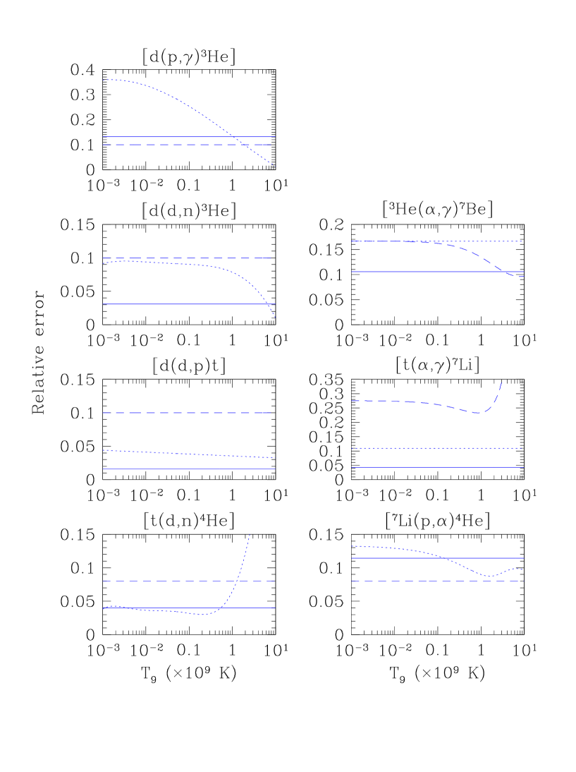
Figure 2: NACRE “high/low” fractional errors for the seven NACRE reactions important for BBN. Dotted curves: high/low errors; solid curves: sample variance errors; dashed curves: SKM errors which are shown for comparison.

We thus turn to the question of assigning statistical meaning of the NACRE high/low limits. The uncertainties are conveniently quantified by the fractional or relative error $\delta_{i}=|\lambda_{i}/\lambda-1|$, with $i=$ high and low In principle, for a given reaction rate the high and low errors need not be equal, but in practice we find that the high and low fractional errors are nearly identical (certainly within our desired accuracy) over the entire temperature range. Thus, we can write the high/low limits as $\lambda_{i}(T)=\lambda(T)\ [1\pm\delta(T)]$, where $\delta=\delta_{\pm}$. This simplifies the analysis slightly. Figure 2 plots the fractional errors $\delta(T)$ for the seven NACRE reactions important for BBN. For comparison, we have also plotted fractional errors given in the SKM compilation. Several trends are apparent in the NACRE curves. We see that in general, the NACRE high/low fractional errors vary with temperature; this is in contrast with the SKM rates, for which only 2 of the 12 rates are assigned a temperature-dependent fractional error.

Comparing the high/low limits with the $1\sigma$ SKM errors, we see that the errors are of the same order of magnitude. There is no clear trend as to which compilation has the larger errors. For example, the NACRE errors for $t(\alpha,\gamma)\mbox{${}^{7}{\rm Li}$}$ are lower than the SKM rates (due in part to the addition of new, accurate data by Brune et al. brune (1994)), while for the mirror reaction $\mbox{${}^{3}{\rm He}$}(\alpha,\gamma)\mbox{${}^{7}{\rm Be}$}$, the NACRE limits are larger than those of SKM. For the purpose of comparison with our more rigorous results which follow, we have taken the simple approach of assigning the NACRE high/low limits to be $1\sigma$ errors. Given the variations in the NACRE rates and their comparison with the SKM variations, this approach is certainly qualitatively correct. A similar approach was taken by Vangioni-Flam, Coc, & Cassé vcc (2000), who examined the impact of the NACRE rates and ran cases using the high/low limits to compare with the central rates.

While the NACRE assignment of limits to their rates invites quantification in a full Monte Carlo code, the somewhat arbitrary nature of the specific assignment of $1\sigma$ errors to the limits leaves question as to the robustness of the results. While here we have assumed a Gaussian distribution for these assignments, other choices such as a log-normal distribution are also possible (Vangioni-Flam, Coc, & Cassé vcc2 (2000)). Thus, we now turn to other error assignments which are derived from the underlying cross section data.

3.3 Minimal Uncertainties: $\Delta\chi^{2}=1$

To derive errors for NACRE rates in a more statistically well-defined way, we now perform our own analysis of data and propagation of errors. In this section, we will treat all cross sections errors, from all data sets, as independent. We thus ignore any correlations between the measurements, even within a given experimental run. Clearly, this is not realistic, but this procedure has the virtue of simplicity and will give the limiting case of the smallest possible error achievable with nuclear data. This will also serve as a useful starting point for a more realistic analysis in the next subsection.

We will compute the variance in the $S$-factor in the form of a fractional error. This is also an approximation, but simplifies the analysis and the limit that results. Physically, this corresponds to the assumption that the large amount of data determines the shape of the curves quite well, so that the dominant uncertainty is not in the shape but in the overall normalization. The data sets used are the same as NACRE; the online versions include data and errors which is greatly helpful in this process.

We can determine the fractional error in the theory fit by varying the normalization until $\chi^{2}=\chi^{2}_{\rm min}+1$, which occurs when

$$\alpha_{1}=\hat{\alpha}\pm\frac{1}{\sqrt{\sum_{i}S_{\rm fit}(E_{i})^{2}/\sigma_{i}^{2}}}$$ (7)

Thus, we have a $1\sigma$ variation when $\alpha$ is changed from its minimizing (renormalized) value by a fractional error

$$f=\alpha_{1}/\hat{\alpha}-1$$ (8)

The theory-data fit thus has a $\pm 1\sigma$ error $\sigma_{\rm th}=f\mbox{${\cal S}_{\rm th}$}=\hat{\alpha}fS_{\rm fit}$.

We have found these “$\Delta\chi^{2}=1$” errors for the 11 strong reactions; these appear in Table 3. In the Table, we see that the errors are very small, $\lesssim 1\%$. This can be seen to follows from the large number of data points. Of course, we have in this case we have assumed each measurement in each experiment to be independent of all others. We have thus ignored the correlations among the errors. These problems are highlighted when we examine the questions of goodness of fit.

The goodness of fit is quantified by $\chi^{2}_{\nu}=\chi^{2}/\nu$, the $\chi^{2}$ per degree of freedom with $\nu=N-1$. Table 2 gives the reduced $\chi^{2}$ for the 11 key strong reactions. For normally distributed and correctly estimated errors, one expects $\chi^{2}_{\nu}$ to lie close to 1. In fact, this is not what is found for any of the reactions. In four cases, the reduced $\chi^{2}$ is significantly less than 1, while in seven cases $\chi^{2}$ significantly exceeds 1. In Figure 1d, we see the data and fit for $t(\alpha,\gamma)\mbox{${}^{7}{\rm Li}$}$, an example of a reaction with $\chi^{2}_{\nu}<1$. In this case, we see that all data are within $1\sigma$ of the fit, and indeed some lie essentially on the fit, leading to the small reduced $\chi^{2}$ and suggesting that the experimental errors may be overly conservative in this case.

For the cases in which $\chi^{2}_{\nu}>1$, we follow the practice of the Particle Data Group and we increase the fractional error by an amount $\sqrt{\chi^{2}_{\nu}}$. This scaling encodes the presumption that at least one of the experiments has underestimated its uncertainties. Where the data are discrepant, this is most assuredly the case. For the cases in which the $\chi^{2}_{\nu}<1$, no correction is made.

Let us examine more closely the large $\chi^{2}_{\nu}$ cases, for which the goodness of fit is poor. A particularly egregious case is $d(p,\gamma)\mbox{${}^{3}{\rm He}$}$, with $\chi^{2}_{\nu}=13.9$, which appears in Figure 1b. The reason for the poor fit is apparent: the data for this reaction are internally inconsistent in the 0.01 to 0.05 MeV range. Specifically, the recent measurements of Schmid et al. schmid (1995) do follow the fit trend, but the older and less precise data of Griffiths, Lal, & Scarfe gls (1963) lie above these data, outside of the range of the quoted errors. In our fitting procedure, the small errors in the Schmid et al. schmid (1995) data dominates the fit normalization, but the systematic offset of the Griffiths, Lal, & Scarfe gls (1963) data leads to a poor $\chi^{2}$.

Another case with a high $\chi^{2}_{\nu}$ is $\mbox{${}^{3}{\rm He}$}(\alpha,\gamma)\mbox{${}^{7}{\rm Be}$}$, which appears in Figure 1c. This reaction has been well-studied in the context of solar models, where it controls the intensity of ${}^{7}{\rm Be}$ neutrinos and thus is of great importance for the solar neutrino problem. Studies of this reaction are reviewed by Adelberger et al. adel (1998), who note the discrepancy between $\gamma$-capture and ${}^{7}{\rm Be}$ activity measurements. Although the discrepancies between the data sets are not as glaring as in the $d(p,\gamma)\mbox{${}^{3}{\rm He}$}$ case, the systematic offset between data sets is nevertheless clear.

The source of the systematic error traces back to the difficulty in making an absolute cross section measurement. While a given experiment can accurately determine the relative values between different energies, measuring the absolute cross section values involves calibration of beam intensities, beam energy losses in the target, detection efficiencies, solid angle uncertainties, etc. Thus, the absolute cross sections from each experiment carry a normalization error, which is common to all points from the experiment. As emphasized by Burles, Nollett, Truran, & Turner bntt (1999) and Nollett & Burles nb (2000), these normalization errors in the cross sections affect all of the BBN reactions, and are properly treated as correlated errors.

Thus, our assumption of independent errors, and the $\Delta\chi^{2}=1$ method, while simple and illustrative, has greatly underestimated the true error budget, in which correlations play an important and even dominant role. We now turn to a method which includes these effects and treats the data in a more uniform manner.

3.4 Sample Variance

We now seek a new error estimator which accounts for correlated errors due to absolute normalization uncertainties in the cross section measurements. These dominate the uncertainties for many reactions. Furthermore, these uncertainties are not reduced by taking more data within a given experiment; rather, each experiment effectively represents one attempt to measure the absolute normalization, independent of the number of points measured in the experiment. Thus, the normalization errors for a given reaction are only lowered by combining many independent experiments. Consequently, the overall error budget in the cross sections, and thus in the inferred thermonuclear rates, is much larger.

We note that the systematic errors in absolute cross section normalization are quoted as percentages. Thus, the use of fractional errors is justified when these errors dominate. We will thus cast our uncertainty determinations in the form of a fractional or normalization uncertainty (as in the previous section), but now with more justification.

In constructing an error estimate which accounts for correlated normalization errors, the data sets with discrepant normalizations will provide a useful test case. Our goal is to find a well-defined procedure which will give errors that automatically account for systematic offsets among data sets, leading to an error range which accommodates both sets. We therefore adopt a (fractional) error determined by the weighted sample variance, as follows. The notation is the same as that introduced in the previous section. In particular, we again adopt a theory normalization $\alpha$ given by $\mbox{${\cal S}_{\rm th}$}=\alpha S_{\rm fit}$, and use the data to determine the value of $\alpha$ and its error. The mean value $\hat{\alpha}$ of the normalization is determined again by $\chi^{2}$ minimization. Given this, we can find the fractional difference

$$\delta_{i}=\frac{S_{\rm obs}(E_{i})-\mbox{${\cal S}_{\rm th}$}(E_{i})}{\mbox{${\cal S}_{\rm th}$}(E_{i})}=\frac{S_{\rm obs}(E_{i})}{\hat{\alpha}S_{\rm fit}(E_{i})}-1$$ (9)

between each data point and the theory, and the fractional error

$$\epsilon_{i}=\sigma_{i}/\mbox{${\cal S}_{\rm th}$}(E_{i})=\sigma_{i}/\hat{\alpha}S_{\rm fit}(E_{i})$$ (10)

in each data point. Given these quantities, the theory normalization $\hat{\alpha}$ which minimizes $\chi^{2}$ (eq. 5) is also the value of $\alpha$ which guarantees that the weighted average theory-data difference satisfies $\langle\delta\rangle=\sum\delta_{i}/\epsilon_{i}^{2}/\sum 1/\epsilon_{i}^{2}=0$. The error, as measured by the weighted sample variance $\sigma_{\alpha}$, is now determined as the weighted average of $\delta_{i}^{2}$:

$$\sigma^{2}_{\alpha}=\frac{\sum_{i}\delta_{i}^{2}/\epsilon_{i}^{2}}{\sum_{i}1/\epsilon_{i}^{2}}=\frac{\sum_{i}\left[S_{\rm obs}(E_{i})-\mbox{${\cal S}_{\rm th}$}(E_{i})\right]^{2}/\sigma_{i}^{2}}{\sum_{i}\mbox{${\cal S}_{\rm th}$}(E_{i})^{2}/\sigma_{i}^{2}}$$ (11)

Note that if a typical data point $S_{\rm obs}$ lies $\sigma$ away from the theory point ${\cal S}_{\rm th}$, then $\sigma_{\alpha}\sim\sigma/\mbox{${\cal S}_{\rm th}$}$, the fractional error. However, since the cross sections are a function of energy and are not constant, the weighting will favor points which have a small fractional error $\sigma_{i}/\mbox{${\cal S}_{\rm th}$}(E_{i})$.

We now turn to the behavior of eq. (11) in the case of discrepant data sets. For a simple but illustrative example, consider a reaction for which there are two data sets which are inconsistent with each other. Let each data set contain $N$ points, with comparable errors. Let the first set have measurements with $S_{\rm obs}(E_{i})=\alpha_{1}S_{\rm fit}(E_{i})+\delta_{i}$ for $i\in(1,\ldots,N)$, so that the data scatters about the fit curve with a normalization discrepancy (systematic error) $\alpha_{1}$, and the errors which scatter as $\langle\delta_{i}\rangle=0$ and $\langle\delta_{i}^{2}\rangle=\sigma_{i}^{2}$. Similarly, the second data set has points with $S_{\rm obs}(E_{i})=\alpha_{2}S_{\rm fit}(E_{i})+\delta_{i}$ for $i\in(N+1,\ldots,2N)$,, where $\alpha_{2}\neq\alpha_{1}$ indicates a systematic discrepancy, and $\langle\delta_{i}^{2}\rangle=\sigma_{i}^{2}$. Finally, as described above, we allow for a theory normalization error: $\mbox{${\cal S}_{\rm th}$}=\alpha S_{\rm fit}$. Then the expected $\langle\chi^{2}\rangle$ is minimized for the normalization

$$\hat{\alpha}=\frac{\sum_{i=1}^{N}S_{\rm fit}{(E_{i})^{2}}/\sigma_{i}^{2}}{\sum_{i=1}^{2N}S_{\rm fit}{(E_{i})^{2}}/\sigma_{i}^{2}}\;\alpha_{1}+\frac{\sum_{i=N+1}^{2N}S_{\rm fit}{(E_{i})^{2}}/\sigma_{i}^{2}}{\sum_{i=1}^{2N}S_{\rm fit}{(E_{i})^{2}}/\sigma_{i}^{2}}\;\alpha_{2}$$ (12)

i.e., a weighted average of the two factors $\alpha_{j}$. This result is of course quite reasonable. In this case, we have

$$\langle\chi^{2}(\hat{\alpha})\rangle=2N+(\Delta\alpha/2)^{2}\sum_{i=1}^{2N}\frac{S_{\rm fit}{(E_{i})^{2}}}{\sigma_{i}^{2}}$$ (13)

We see that $\chi^{2}$ differs from the number $\nu=2N-1\sim 2N$ of degrees of freedom by an amount which depends on $\Delta\alpha$, the difference in the systematic error. In this case, therefore, the degree to which $\chi^{2}$ exceeds $\nu$, or $\chi^{2}_{\nu}$ exceeds 1, is just a measure of the systematic discrepancy between the data sets. Again, this is as expected.

For the special case when $S_{\rm fit}=S_{0}$ and $\sigma_{i}=\sigma_{0}$, both constants independent of energy, eq. (12) reduces to just $\hat{\alpha}=(\alpha_{1}+\alpha_{2})/2$, the simple average. Furthermore, in this case the weighted sample variance of eq. (11) takes the simple form

$$\sigma_{\alpha}^{2}=(\sigma_{0}/S_{0})^{2}+(\Delta\alpha/2)^{2}$$ (14)

where $\Delta\alpha=\alpha_{2}-\alpha_{1}$. Again, this result is quite reasonable: the fractional error in the normalization is the quadrature sum of a typical fractional measurement error $\sigma_{0}/S_{0}$ and the systematic error as estimated by $(\alpha_{2}-\alpha_{1})/2$, the difference in normalizations. Thus, when the systematic error dominates, then $\sigma_{0}/S_{0}\ll\Delta\alpha$ we have an overall fractional error $\sigma_{\alpha}\simeq\Delta\alpha/2$, so that the range $\alpha=\hat{\alpha}\pm\sigma_{\alpha}$ corresponds precisely to the range $\alpha_{1}\leq\alpha\leq\alpha_{2}$. This is precisely what one expects if the systematic error dominates; our expression automatically gives an answer which spans the range between the discordant data sets. On the other hand, if the systematic error is negligible, then we have $\sigma_{0}/S_{0}\gg\Delta\alpha$, and $\sigma_{\alpha}\simeq\sigma_{0}/S_{0}$, a typical measurement error. In this limit, then, the fractional error is such that it encloses the $1\sigma$ error band about the (normalized) fit curve.

Table 3: Reaction Errors

	Minimal Error	Sample Variance	SKM fractional
Reaction	$f$	$\sigma_{\alpha}$	error
$d(p,\gamma)\mbox{${}^{3}{\rm He}$}$	0.00420	0.132	0.10
$t(d,n)\mbox{${}^{4}{\rm He}$}$	0.00233	0.0401	0.08
$d(d,n)\mbox{${}^{3}{\rm He}$}$	0.00176	0.0310	0.10
$d(d,p)t$	0.00077	0.0159	0.10
$t(\alpha,\gamma)\mbox{${}^{7}{\rm Li}$}$	0.0145	0.0421	$\sim 0.23-0.30$ ($T$-dep)
$\mbox{${}^{3}{\rm He}$}(\alpha,\gamma)\mbox{${}^{7}{\rm Be}$}$	0.0068	0.106	$\sim 0.10-0.17$ ($T$-dep)
$\mbox{${}^{7}{\rm Li}$}(p,\alpha)\mbox{${}^{4}{\rm He}$}$	0.0059	0.114	0.08
$\mbox{${}^{3}{\rm He}$}(n,p)t$	0.00467	0.03523	0.10
$\mbox{${}^{3}{\rm He}$}(d,p)\mbox{${}^{4}{\rm He}$}$	0.00699	0.0915	0.08
$p(n,\gamma)d$	0.00324	0.0445	0.07
$\mbox{${}^{7}{\rm Be}$}(n,p)\mbox{${}^{7}{\rm Li}$}$	0.00621	0.0387	0.09

Table 3 shows $\sigma_{\alpha}$ for the 11 strong BBN reactions. We see that these results are either comparable to or smaller than the SKM results. The largest uncertainties appear when incompatible data sets are present. As expected, the systematic offsets are accounted for by an increase in the errors.

3.5 Other BBN Error Studies

Other studies have been made which determine errors in the nuclear inputs for BBN and propagate them to derive uncertainties in BBN abundance predictions. The SKM compilation of nuclear uncertainties has been very widely used for BBN Monte Carlo studies. This work was extremely influential, as it was the first to catalog the most important BBN reactions, to systematically collect, and display the available cross section data for them, and to derive a set of errors for them. The explicit table of uncertainties (given as fractional errors) made the SKM work very useful, as these that could be readily input into BBN codes.

An important recent study takes a very different approach to the BBN error budget. Burles, Nollett, Truran, & Turner bntt (1999) and Nollett & Burles nb (2000) made an extensive Monte Carlo calculation of the light element abundances and their uncertainties. In this work, the $R$- and $S$-factors for the 11 key strong reactions are generated from fits to simulated data sets. These mock data are drawn randomly, on the basis of the actual data. For each realization of the nuclear data, the thermonuclear rates are computed via eq. (1), and run in the BBN code. Care is taken to allow for correlations due to normalization errors. We note however, that there is a danger in this procedure, as the resulting adopted $S$ and $R$- factors may not have a dependence as a function of energy as expected from theory. Indeed, some cases, such as ⁷Li(p,$\alpha$)⁴He, show a behavior which is probably not physical and is simply a result of the available data at particular energies

Thus, Nollett & Burles do not directly report a mean and error for the thermonuclear rates (though they do produce mean values and errors for the $R$- and $S$-factors). Instead, they report the final results for the abundance mean values and errors, as a function of $\eta$. Finally, we note that Nollett & Burles adopt a neutron lifetime $\tau_{n}=885.4\pm 2$ s, which is slightly lower than the current world average of the Particle Data Group (Groom et al. 2000), $885.7\pm 0.8$ s. This difference affects mostly ${}^{4}{\rm He}$, with a small drop $\Delta Y_{p}\simeq-0.0001$ for the Burles & Nollett value, although the error used here is considerably smaller.

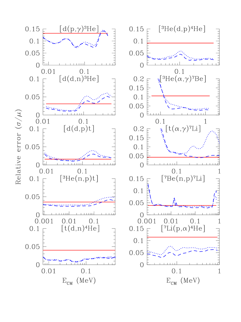
Figure 3: Fractional $1\sigma$ errors in the $R$- and $S$-factors for sample variance analysis, as well as Nollett & Burles nb (2000). Solid curves: sample variance limits; dashed curves: Nollett & Burles upper limits; dotted curves: Nollett & Burles lower limits. The $p(n,\gamma)d$ reaction is not shown, as Nollett & Burles adopt a constant $1\sigma$ fractional error of 5% in this case.

To compare our nuclear error budgets with those of SKM and Nollett & Burles nb (2000), we have plotted fractional errors in the $R$- and $S$-factors for 10 of the 11 strong reactions. These appear in Figure 3. We see that our sample variance uncertainties are always tighter than those of SKM. On the other hand, our results are almost always larger than or about equal to the errors found by Nollett & Burles. It is interesting that, with the exception of the two $(\alpha,\gamma)$ reactions, the Nollett & Burles fractional errors are roughly constant with energy. In four of these cases, our values agree well with the average of the range spanned by Nollett & Burles. For $d(p,\gamma)\mbox{${}^{3}{\rm He}$}$, our value is slightly higher, due to method’s slightly more conservative treatment of the discrepant data for this reaction as is the case for $\mbox{${}^{7}{\rm Li}$}(p,\alpha)\mbox{${}^{4}{\rm He}$}$. In the mirror reactions of $t(d,n)\mbox{${}^{4}{\rm He}$}$ and $\mbox{${}^{3}{\rm He}$}(d,p)\mbox{${}^{4}{\rm He}$}$, the reactions proceed through a resonance, and thus the errors are very sensitive to the goodness of fit for the NACRE and SKM curves, which is not an issue for the empirical approach of Nollett & Burles.

4 The Impact on BBN

We have now adopted a set of thermonuclear rates using the NACRE compilation (§2), and we have presented several estimates of the uncertainties in theses rates (§3). In this section, we will put these rates into the BBN code, and compute the light element abundances and their errors as a function of $\eta$. We can then quantify the impact of the NACRE compilation on the mean values of the abundances, and on their uncertainties.

The implementation of the Monte Carlo is standard and well-described in, e.g., Krauss & Romanelli kr (1990) and SKM. Briefly, a grid of $\eta$ is chosen, with values in the $(1-10)\times 10^{-10}$ range. At each $\eta$, the code is run 1000 times. For each run, we generate 12 Gaussian random numbers $z_{i}$ with zero mean and unit variance; these are used to choose the thermonuclear reaction rates $\lambda_{i}$ in terms of their mean values $\lambda_{i,0}$ and fractional errors $f_{i}=\delta\lambda_{i}/\lambda_{i,0}$:

$$\lambda_{i}(T)=\lambda_{i,0}(T)\ \left[1+z_{i}f_{i}(T)\right]$$ (15)

Where $f_{i}(T)$ is constant for the minimal uncertainty and sample variance cases, and $T$-dependent for the high/low case.

At each $\eta$, the central value of the light element abundance $\hat{y_{i}}$ is taken to be the mean of the 1000 values from the runs, and the standard deviation $\sigma(y_{i})$ is taken from the sample variance of the 1000 runs. A technical note: the sample variance itself has an expected deviation of $\delta\sigma^{2}\sim\sigma^{2}/N$ from the true error, so that our uncertainty estimates have a statistical error of $1/\sqrt{N}\simeq 3\%$. To allow for this, we increase the computed sample variance by 3%; in every case the effect is small.

4.1 NACRE Central Values

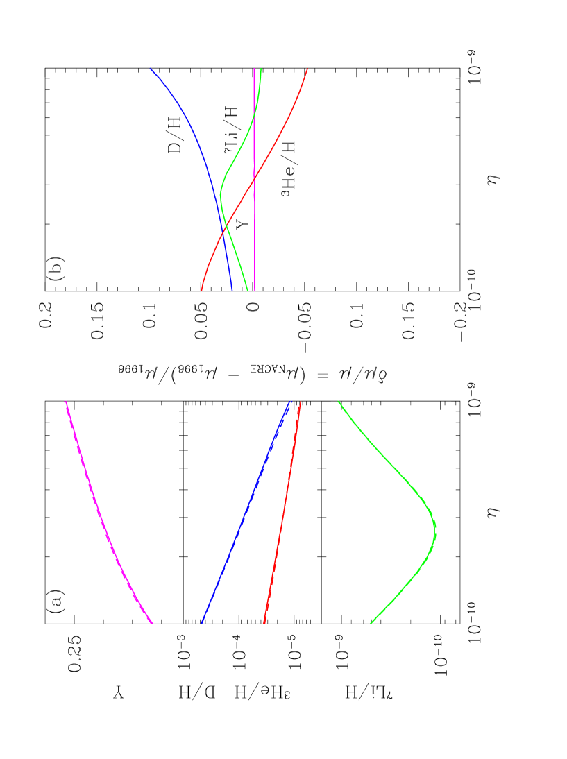
Figure 4: Light element abundances as a function of $\eta$, using NACRE rates without renormalization. a) The solid curves are the central values of the NACRE predictions, dashed curves are those of SKM. The two are extremely close, so that they often appear to overlap. b) Percent difference $100(y_{i}^{\rm NACRE}/y_{i}^{\rm 1996}-1)$ between the NACRE and Hata et al. (1996) central values.

It is important to first compare the direct impact of the NACRE rate compilation on BBN predictions. To do this we will use the expanded BBN code of Thomas et al. (1993), which was based on the Kernan (1993) code, with the Monte Carlo implemented by Hata et al. (1996). The uncertainties in the 1996 Monte Carlo were derived from SKM. The central values of the light element abundances appear in Figure 4a, which shows results for the NACRE rates along with the Hata et al. (1996) results. (the solid and dashed curves). We see that the two predictions are almost identical to each other. The differences between the two cases are plotted in Figure 4b as a percentage of the 1996 predictions. We see that the changes are small: the largest shift is a 10% rise in D/H at $\eta=10^{-9}$, and that below $\eta=3\times 10^{-10}$, all shifts are smaller than 5% in magnitude.

These results confirm the findings of Vangioni-Flam, Coc, & Cassé vcc (2000): the central values of the BBN predictions are insensitive to the reaction network choice. It is both non-trivial and comforting that different rate tabulations, with different functional forms, yield the same central values. This agreement reaffirms that basic predictions of BBN are robust.

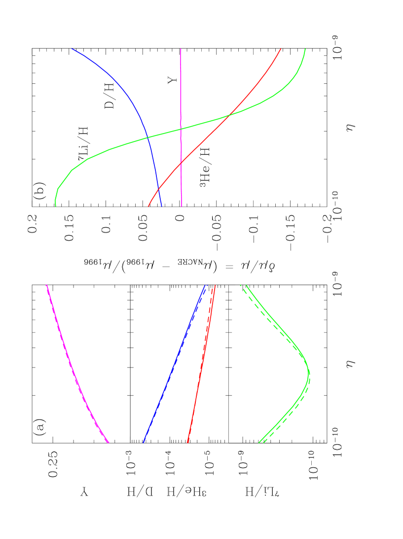
Figure 5: As in Figure 5, for light element predictions with renormalization.

Although the central light element predictions of the two rate compilations do not differ significantly, a larger effect is found by renormalizing the rates to reflect the data in the BBN energy range. Figure 5a shows the predictions when the rates are renormalized as described in the previous section. We see that central values do change, at levels larger than those discussed above. Figure 5b shows the percent difference of these predictions with those of Hata et al. (1996). We see that the shifts are $\ll 1\%$ for $Y_{p}$, at a level of $\leq 15\%$ for D and ${}^{3}{\rm He}$, and vary the most for ${}^{7}{\rm Li}$, which runs between $\pm 20\%$. The shifts trace back to the rates which have the largest renormalizations. In particular, the $d(p,\gamma)\mbox{${}^{3}{\rm He}$}$ rate drops by 7.6% with respect to NACRE due to the preferential weighting of the Schmid et al. schmid (1995) data with their smaller errors (Figure 1d). This change alone is predominantly responsible for the shifts in D, ${}^{3}{\rm He}$, and ${}^{7}{\rm Li}$ at $\eta\gtrsim 3\times 10^{-10}$; the $\mbox{${}^{3}{\rm He}$}(d,p)\mbox{${}^{4}{\rm He}$}$ +6.9% renormalization is responsible for most of the rest of the shift in this regime. At smaller $\eta$, there is a rise in ${}^{7}{\rm Li}$; this is predominantly due to the combination of the increase in ${}^{7}{\rm Li}$ production via a 5.8% rise in the $t(\alpha,\gamma)\mbox{${}^{7}{\rm Li}$}$ rate, and a decrease in ${}^{7}{\rm Li}$ destruction due to a 4.5% lowering of the $\mbox{${}^{7}{\rm Li}$}(p,\alpha)\mbox{${}^{4}{\rm He}$}$ rate. We note that these shifts in the central values of the predicted abundances are well within the calculated uncertainties discussed below.

4.2 NACRE High/Low Errors

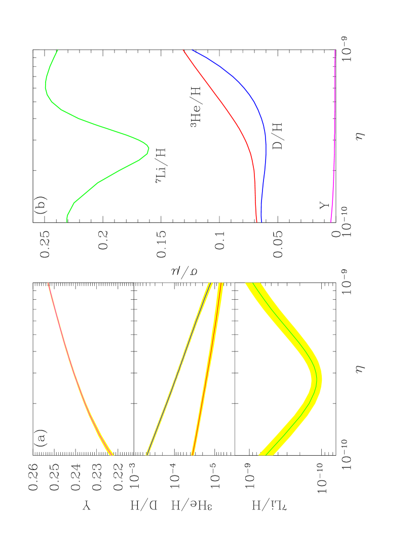
Figure 6: Light element abundance predictions, and their uncertainties, as a function of $\eta$. a) The solid curves are the (renormalized) NACRE abundance predictions, and the broken curves are the $1\sigma$ Monte Carlo errors for the NACRE high/low error estimates. b) The fractional errors in the light element predictions, for the NACRE high/low estimates as in (a) (solid curves). The fractional errors plotted are $\sigma_{i}/\mu_{i}$, where $\mu_{i}$ is the mean value of abundance $i$, and $\sigma_{i}$ is its error.

The impact of NACRE’s high/low errors (§3.2) on the light element abundances is seen in Figure 6a. The logarithmic nature of the standard abundance plot, and the rapid variation of the trace elements, makes it difficult to assess and compare the errors. Thus we have also plotted the fractional errors $\sigma_{i}/\mu_{i}$ in Figure 6b. We see that overall, the NACRE high/low errors are quite comparable to those found using the SKM estimates. The most significant effect is the reduction in the ${}^{7}{\rm Li}$ errors, which is due to the lower uncertainties in the mass-7 production reactions $t(\alpha,\gamma)\mbox{${}^{7}{\rm Li}$}$ and $\mbox{${}^{3}{\rm He}$}(\alpha,\gamma)\mbox{${}^{7}{\rm Be}$}$. Here, the errors are a strong function of $\eta$ owing to the ${}^{7}{\rm Li}$ and ${}^{7}{\rm Be}$ production channels, and the errors are comparable to those of SKM at $\eta_{10}=10^{10}\eta$ near 3. However, the error on Li is reduced by as much as $\sim 25\%$ for $\eta_{10}$ near 1 or 10,

We confirm here the key result that the theoretical errors in BBN are still significant. The errors in D and ${}^{7}{\rm Li}$ in particular are only marginally smaller than the accuracy of current or near-future observations. Thus, improvements in the nuclear inputs to BBN can still have an important effect on cosmology, as we will discuss below (§5.3).

It is important to note that our results differ somewhat from those of Vangioni-Flam, Coc, & Cassé vcc (2000), due to differences in approach. Vangioni-Flam et al. used the high/low errors to examine the effect on BBN of each reaction individually. They then found the abundances when all the reactions are set to their high limits, then when all reactions are set to their low limits. This procedure is a simple and rapid means of gauging the net effect of the uncertainties. However, as Vangioni-Flam et al. note, this can lead to compensating effects (e.g., since both the ${}^{7}{\rm Li}$ destruction and production rates are raised, there is a degree of cancellation in the effect of the errors on the final abundances). Thus, the Vangioni-Flam et al. net uncertainties are lower limits to the true uncertainties; this fact is borne out in Figures 6a and 6b, where the errors are equal to or larger than those of Vangioni-Flam et al.

4.3 Minimal Uncertainties: $\Delta\chi^{2}=1$

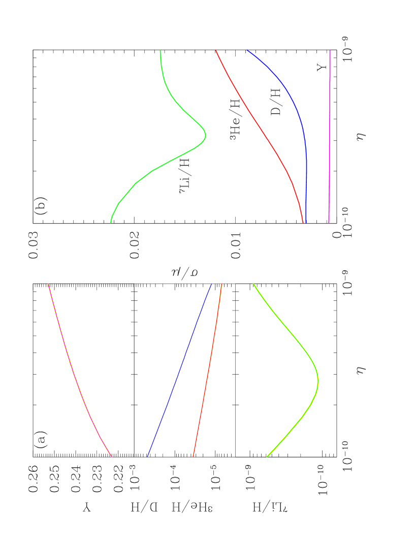
Figure 7: As in Figure 6, with errors for the $\Delta\chi^{2}=1$, “minimal uncertainty” estimates. Note the change in vertical scale between panel (b) and Figure 6b.

We now turn to the case of the uncertainties given in the $\Delta\chi^{2}=1$ analysis of §3.3. Results appear in Figure 7, where we see that the errors are now very small. This is not a surprise, given that these errors represent a lower limit to the true uncertainties. In this limit, the nuclear input errors are small enough to be negligible in comparison to the uncertainties one can expect in the observed abundances.

The errors presented here are derived by assuming that all of the cross section data points may be combined without concern for systematic errors between the experiments. As this is not likely to be the case, the true BBN theoretical error budget is considerably larger, however. We now turn to the “sample variance” error estimator, which allows for these effects.

4.4 Sample Variance

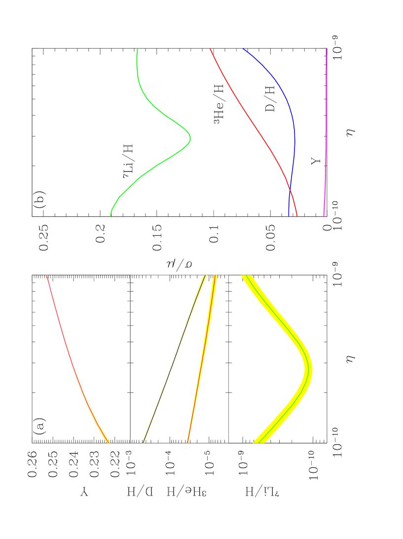
Figure 8: As in Figure 6, with sample variance error estimates.

The BBN predictions based on the sample variance errors appear in Figure 8. The smallest errors are of course for ${}^{4}{\rm He}$, where the uncertainties are of order $\sim 2\%$, or $\Delta Y=0.0005$. We note that the neutron lifetime is now sufficiently well-known that the prediction for ${}^{4}{\rm He}$ are now dominated instead by the nuclear errors. The D/H errors are also of the same order as the statistical errors in the (high-redshift) data, though systematics are likely to dominate the observational uncertainties, as discussed in the next section.

The largest errors are for ${}^{7}{\rm Li}$, where the $\sim 10-18\%$ uncertainty is of the same order of the statistical error in the observations. Again, systematic errors are more important for the observations. Even so, it is particularly important to reduce the error in Li regardless of the uncertainty in the observations. As noted by, e.g., Ryan et al. rbofn (2000), since the interesting range in $\eta$ places the Li($\eta$) curve near its minimum, it is therefore slowly varying. Even if there are zero observational errors, the shallowness of the $\mbox{${}^{7}{\rm Li}$}-\eta$ curve means that the theoretical uncertainty in the Li prediction leads to a large error in the allowed range for $\eta$ (below, §5).

We now compare the errors derived from the sample variance with the other estimators we have used. Referring to the panels (b) of Figures 8, 6, and 7, we see that the sample variance errors are smaller than those using SKM, or NACRE’s high/low ranges, but larger than the minimal errors, as expected. Relative to SKM, the Li errors are reduced on the low-$\eta$ side (i.e., the ${}^{7}{\rm Li}$ regime) by the inclusion of the precision $t(\alpha,\gamma)\mbox{${}^{7}{\rm Li}$}$, data of Brune, Kavanagh, & Rolfs brune (1994). On the high-$\eta$ side, the reduced Li errors follow from our smaller errors in $\mbox{${}^{3}{\rm He}$}(\alpha,\gamma)\mbox{${}^{7}{\rm Be}$}$. The ${}^{3}{\rm He}$ and D errors are considerably lower (by roughly a factor $\sim 2$), due to the smaller errors in $p(n,\gamma)d$, $d(d,n)\mbox{${}^{3}{\rm He}$}$, and $d(d,p)t$.

Of the error estimation methods we have used, we feel the sample variance method provides a good and fair estimate of BBN uncertainties. This procedure has the virtue of allowing for systematic uncertainties due to reaction normalization errors. It also has the virtue of simplicity of definition and implementation, and one can judge by eye the goodness of the fit.

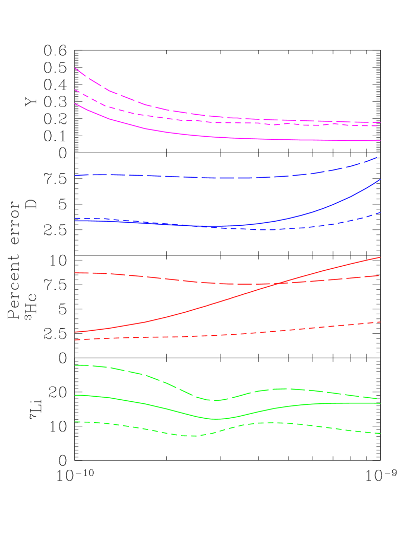
Figure 9: A comparison of BBN fractional errors by different groups. Solid curves show our sample variance errors for the four light elements, short dashed curves are the errors from Nollett & Burles nb (2000), and long dashed curves are the errors from SKM. We see that our errors generally fall between these two cases.

The sample variance errors are compared with those of Nollett & Burles nb (2000) and SKM in Figure 9. The differences among the fractional errors plotted stem mostly from differences in the errors $\sigma_{i}$ themselves, except for the case of ${}^{7}{\rm Li}$, where the differences in central values $\mu_{i}$ (ours are lower than those of SKM and NB) also contribute to changes in $\sigma/\mu$. We see in Figure 9 that our relative errors generally lie between those of SKM and Nollett & Burles. This is as expected, since the NACRE thermonuclear rates, normalized or not, follow similar trends to those rates used by SKM and Nollett & Burles. Also, our sample variance usually lies between those of SKM and Nollett & Burles’ errors. For each element, different reactions dominate the errors at different regimes in $\eta$, and thus the variations of the shapes of the curves in each panel of Figure 9 reflect the differences in the underlying reaction errors. As seen in Figure 3 and Table 3, both the SKM and Nollett & Burles errors are generally of comparable magnitudes across most reactions; ours have somewhat larger variations in magnitudes, and thus our curves have a somewhat different $\eta$ dependence than those of these compilations.

For example, in comparison with Nollett & Burles, we find that the D/H fractional errors are in very good agreement for $\eta_{10}\lesssim 3$. At higher $\eta$, our errors then grow larger, about 30% larger at $\eta_{10}=5$, to 80% larger at $\eta_{10}=10$; this difference is mostly due to the increasing sensitivity of deuterium to the $d(p,\gamma)\mbox{${}^{3}{\rm He}$}$ rate, for which our adopted error is larger. The trend for ${}^{3}{\rm He}$ shows a more pronounced rise at higher $\eta$, due to the increasing importance of both the $d(p,\gamma)\mbox{${}^{3}{\rm He}$}$ and $\mbox{${}^{3}{\rm He}$}(d,p)\mbox{${}^{4}{\rm He}$}$ rates, where again we have used a larger uncertainty.

For ${}^{7}{\rm Li}$, our errors are consistently higher, by a factor that varies from 70% to 100%; part of this difference arises from the somewhat higher central values Nollett & Burles have at higher $\eta$ (and thus a smaller $\sigma/\mu$). The rest of the differences trace back to the systematically tighter Nollett & Burles error bands, as discussed above. The difference does not stem from a single reaction, but rather the cumulative effect of the lower Nollett & Burles errors for several reactions: $d(p,\gamma)\mbox{${}^{3}{\rm He}$}$, as well as the mass-7 producing and destroying reactions. In the case of $Y$, our errors are smaller than those of the other groups; this arises because we have adopted the new errors in the neutron mean life which are smaller than those used by Nollett & Burles and others in the past.

5 Comparison with Observation

The procedure for comparing the light element abundances as predicted by BBN theory with the light elements as observed astrophysically is well-described elsewhere, e.g., (Olive, Steigman, & Walker osw00 (2000)). Here, we simply summarize the needed observational inputs and statistical techniques.

5.1 Observational Inputs

Data for ${}^{4}{\rm He}$ is available from about 70 extragalactic H II regions (Pagel et al. 1992; Skillman & Kennicutt 1993; Skillman et al. 1994; Izotov, Thuan, & Lipovetsky 1994,1997; Izotov & Thuan 1998b) and has been recently compiled in Olive, Steigman, & Skillman oss (1997) and Fields & Olive fdo2 (1998). Unfortunately, the determination of the ${}^{4}{\rm He}$ abundance in these systems is not particularly straightforward. To convert the observed He emission line strengths into abundances requires knowledge of several physical parameters describing the H II system, such as the temperature, electron density, optical depth, and degree of underlying stellar absorption.

The older data of Pagel et al. (1992), Skillman & Kennicutt (1993), and Skillman et al. (1994), used S II data to fix the electron density from which was derived a relatively low ${}^{4}{\rm He}$ abundance. Higher ${}^{4}{\rm He}$ abundances were derived by Izotov, Thuan, & Lipovetsky (1994,1997) and Izotov & Thuan (1998b), where the electron density was determined self consistently from five distinct He emission lines. In addition, it was pointed out in Izotov & Thuan (1998a) that one of lowest metallicity regions, I Zw 18 NW, is plagued by underlying stellar absorption. The compilation by Izotov & Thuan (1998b) of 45 extragalactic H II regions yielded a primordial ${}^{4}{\rm He}$ abundance (by performing a regression on the data versus the O/H abundance) of $Y_{p}=0.244\pm 0.002$. As the compilation of Izotov & Thuan (1998b) also presented results based on S II densities, it was possible to combine all of the data in a systematic way. The result of Fields & Olive fdo2 (1998) which included the data of Pagel et al. (1992), Skillman & Kennicutt (1993), and Skillman et al. (1994) and Izotov & Thuan (1998b) (but without the possibly erroneous I Zw 18 NW), yielded the somewhat lower result of $Y_{p}=0.238\pm 0.002$. Note that the data of Izotov & Thuan (1998b) alone based on S II densities give $0.239\pm 0.002$. One should also note that a recent determination by Peimbert, Peimbert, & Ruiz (2000) of the ${}^{4}{\rm He}$ abundance in a single object (the SMC) also using a self consistent method gives a primordial abundance of 0.234 $\pm$ 0.003 (actually, they observe $Y=0.240\pm 0.002$ at the relatively high value of [O/H] = -0.8, where [O/H] refers to the log of the Oxygen abundance relative to the solar value).

Recently, a detailed examination of the systematic uncertainties in the ${}^{4}{\rm He}$ abundance determination was made by Olive & Skillman (2000). There a Monte Carlo simulation of synthetic data showed that the He abundance determinations using a $\chi^{2}$ minimization in the self-consistent method typically under-estimated the true errors by about a factor of 2. The reason for the enhanced error determinations is a degeneracy among the physical parameters (electron density, optical depth, and underlying stellar absorption) which yield equivalent $\chi^{2}$ results. Indeed, it was found that there are competing biases in the data. On the one hand, the presence of underlying stellar absorption (expected to be present to some level in most systems) leads to an underestimate of the He abundance. While on the other hand, the minimization solutions tend to find solutions with erroneously low densities thus minimizing the collisional corrections and over-estimating the He abundance.

With these cautions in mind, we will never-the-less adopt the Fields & Olive fdo2 (1998) value of

$$Y_{p}=0.238\pm 0.002\pm 0.005$$ (16)

where the first error is statistical and the second systematic. Clearly, the dominant error source is systematic, and while we have given our best estimate for its value, this number may yet turn out to be too small until a complete reanalysis of the existing or new data is possible. For the full error in $Y_{p}$, we will use the quadrature sum of the two components.

As in the case of ${}^{4}{\rm He}$, there is a considerable body of data on ${}^{7}{\rm Li}$. There are well over 100 hot halo dwarf stars with ${}^{7}{\rm Li}$ observations. The discovery of a plateau in the Li abundance for hot and metal poor dwarfs by Spite & Spite (1982), is generally recognized as the primordial value. Recent high precision studies of Li abundances in halo stars have been made by Bonifacio & Molaro (1997) and Ryan, Norris, & Beers rnb (1999) which confirm the plateau. The latter in fact identified a small but significant Li-Fe trend in the low metallicity regime. Ryan et al. rbofn (2000) showed that this trend is indeed expected given the presence of cosmic ray interactions in the early Galaxy. These provide a source of Galactic Li production on top of a cosmological value (very analogous to the derivation of $Y_{p}$ from a regression of $Y-Z$ data and the $dY/dZ$ slope). Ryan et al. inferred a primordial Li abundance of

$$\mbox{${}^{7}{\rm Li}$}/{\rm H}=(1.23^{+0.68}_{-0.32})\times 10^{-10}$$ (17)

Note that correcting for Galactic production lowers ${}^{7}{\rm Li}$/H compared to taking the mean value over a range of metallicity. For our adopted primordial ${}^{7}{\rm Li}$, we assume a gaussian distribution with central value equal to that of eq. (17), and a standard deviation which we conservatively take to be the larger of the asymmetric errors.

We note that in contrast to the downward correction due to post big bang production of Li, there is a potential for an upward correction due to depletion. While most studies of possible depletion factors are small, they may not be negligible. Both Vauclair & Charbonnel vc (1998) and Pinsonneault et al. (1998) argue for an upward correction of 0.2 dex. We note however, that the data do not show any dispersion (beyond that expected by observational uncertainty) and both Bonifacio & Molaro (1997) and Ryan, Norris, & Beers rnb (1999) have argued strongly against depletion. We further point out that the observation of the fragile isotope, ${}^{6}{\rm Li}$, (Smith, Lambert & Nissen 1992, 1998; Hobbs and Thorburn 1994, 1997, Cayrel et al. 1999; Nissen et al. 2000) also puts strong constraints on the degree of depletion (Steigman et al. 1993; Lemoine et al. 1997; Fields & Olive 1999; Vangioni-Flam et al. 1999).

The observational status of primordial D is complicated but also promising. Deuterium has been detected in several high-redshift quasar absorption line systems. It is expected that these systems still retain their original, primordial deuterium, unaffected by any significant stellar nucleosynthesis. At present, however, there are four good determinations of D/H in absorption systems with considerable scatter. Two good measurements (Burles & Tytler 1998a ; 1998b ) with D/H determinations of D/H = $(3.3\pm 0.3)\times 10^{-5}$ and $(4.0\pm 0.7)\times 10^{-5}$, have recently been supplemented by the new results of O’Meara et al.  omera (2000) with D/H = $(2.5\pm 0.2)\times 10^{-5}$. These authors measured D/H in a Lyman limit system which has a neutral hydrogen column density a factor of 30–100 higher than the previous D/H systems, and in which most of the H is neutral rather than ionized. As a result, O’Meara et al.  omera (2000) were able to detect D in five transitions. The inferred D/H value is lower than the previous absorption systems, and the three systems combined give

$${\rm D/H}=(3.0\pm 0.4)\times 10^{-5}$$ (18)

O’Meara et al.  omera (2000) note, however, that $\chi^{2}_{\nu}=7.1$ for the combined 3 D/H measurements (i.e., $\nu=2$), and interpret this as a likely indication that the errors have been underestimated.

Significantly more discrepant is the higher determination of D/H, $(2.0\pm 0.5)\times 10^{-4}$, as seen in one low-redshift system (Webb et al. webb (1997); Tytler et al. tytler (1999)). Clearly there are systematic uncertainties which are yet to be sorted out. Indeed, Levshakov, Kegel & Takahara (1998) have used the data in the high redshift system of Burles & Tytler 1998a but with a different model for the velocity distribution of the absorbing gas, and derived a 95% confidence range 3.5 $\times 10^{-5}\leq$ D/H $\leq 5.2\times 10^{-5}$. Levshakov, Tytler & Burles lev (1998) have also applied this model to a reanalysis of the system of Burles & Tytler 1998b , finding a a 68% confidence range of D/H $\simeq(3.5-5.0)\times 10^{-5}$. Because of these complications, we will examine the impact of low and high D on BBN.

5.2 Likelihood Analysis

To quantitatively compare the observed abundance data with theory, we use a likelihood analysis. The formalism is described elsewhere (Fields & Olive fdo1 (1996); Fields, Olive, Kainulainen, & Thomas fkot (1996)), but the basic idea is that the Monte Carlo results (means, variances, correlation coefficients) allow one to compute the theory likelihoods for the elements as a function of $\eta$. The convolution of these with the observed abundance distributions gives the overall likelihood as function of $\eta$; these can determine the goodness of fit of the model and allow for parameter estimation.

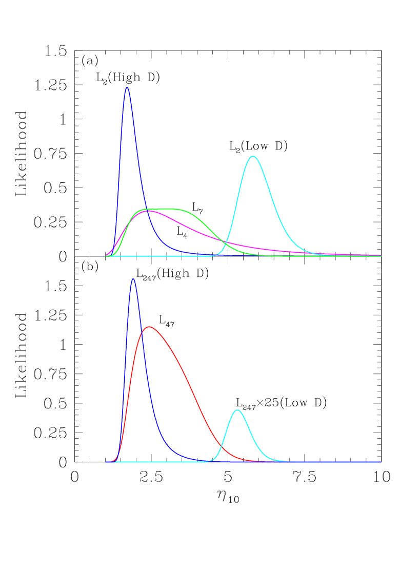
Figure 10: Likelihoods for the sample variance errors. a) Curves for ${}^{4}{\rm He}$ and ${}^{7}{\rm Li}$, as well as high and low D individually. Plotted are the likelihoods for combined theory and observation distribution. The small amplitude for the low D case indicates a poorer fit. b) Total 2- and 3-element combined likelihoods.

Figure 10 shows the likelihoods derived using the sample variance errors. In panel (a), we see the theory-observation combined distributions for individual elements. The peaked nature of the ${}^{4}{\rm He}$ and D curves stems from the monotonic nature of the $\eta$ dependence of these abundances. The flatness of the ${}^{7}{\rm Li}$ likelihood arises because the observed ${}^{7}{\rm Li}$ abundance we have adopted lies at the minimum of the lithium trough, so that the usual two-peaked structure has merged into a single broad feature. As has noted in Fields et al.  fkot (1996) and elsewhere, the ${}^{4}{\rm He}$ and ${}^{7}{\rm Li}$ likelihoods are in excellent agreement with each other and with the high D distribution. This is reflected in the combined likelihood distribution (panel b). Here, $L_{47}$ represents the combined likelihood distribution using only ${}^{4}{\rm He}$ and ${}^{7}{\rm Li}$, while $L_{247}$ is the combined likelihood distribution using D, ${}^{4}{\rm He}$ and ${}^{7}{\rm Li}$. A value of order unity is an indication that the agreement is good.

On the other hand, the low D distribution agrees marginally at best with the ${}^{4}{\rm He}$ and ${}^{7}{\rm Li}$ data. This discrepancy has been widely noted, and if real, suggests that either one or more of the observed abundances is incorrect, that the systematic uncertainties have been grossly underestimated, or perhaps that new physics is at play. One should recall, though, that the D observations could as well suffer from systematic errors that are not reflected in numbers we have adopted. Indeed, systematic uncertainties are not included in the error budget of eq. (18). Since D/H is a strong function of $\eta$, the D likelihood distribution is very sensitive to changes in the D data; for example, a modest shift upward in the D central value, or a larger D error, could lead to agreement with ${}^{4}{\rm He}$ and ${}^{7}{\rm Li}$. For example, even if D/H is only as high as $\sim 5\times 10^{-5}$, as deemed possible in the mesoturbulent models of Levshakov, Kegel & Takahara (1998) and Levshakov, Tytler & Burles lev (1998), the peak of the likelihood function shifts down to $\eta_{10}\approx 4$ and would indeed be in good agreement with the other light elements. As is also well known, the high D/H distribution is in excellent agreement as seen in Fig. 10. Clearly, a determination of the true, primordial D abundance–and an accurate assessment of its errors—is of paramount importance.

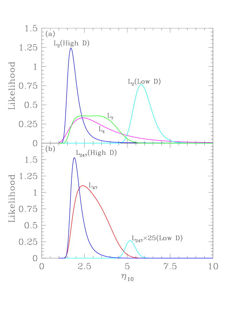
Figure 11: Likelihoods as in Figure 10 for the minimal errors.

Had we used the high/low errors of the NACRE rates we would have obtained very similar likelihood distributions and predictions for $\eta$. Similarly, the use of the unrenormalized rates would not have made a big difference here either. In the extreme case that we use our minimal uncertainties based on $\Delta\chi^{2}=1$, we would of course have tighter predictions as shown in Figure 11. It is interesting to note that even in this case, the likelihood distributions for ${}^{4}{\rm He}$ and ${}^{7}{\rm Li}$ are broad due to residual systematic uncertainties in the observations. Therefore, for any significant improvement in the BBN predictions, the systematic uncertainties will need to be resolved.

5.3 Constraints on Cosmology: The Baryon Density and Light Neutrinos

Using the results of the likelihood analyses in the previous section, we can derive limits on $\eta$. We will focus on the sample variance case; as we have remarked, the likelihoods for the high/low case are only slightly different, and we have verified that they give very similar results for $\eta$.

For the sample variance error, we derive a most-likely value of $\eta$, $\hat{\eta}$, and a 95% CL range. For the ${}^{4}{\rm He}$-${}^{7}{\rm Li}$ combined likelihood, we find (to two significant digits)

$$\hat{\eta}_{10}=2.4 \Rightarrow \hat{\Omega}_{\rm B}h^{2}=0.0089$$ (19)

$$1.7\leq{\eta_{10}}\leq 4.7 \Rightarrow 0.006\leq\Omega_{\rm B}h^{2}\leq 0.017\ \ \ \mbox{(95\% CL) \ .}$$ (20)

where $\hat{\eta}$ is the value at maximum likelihood. We use the conversion $\eta_{10}=274\Omega_{\rm B}h^{2}$. For high D, the result is very similar, owing to the close overlap of the individual element likelihoods; we have

$$\hat{\eta}_{10}=1.9 \Rightarrow \hat{\Omega}_{\rm B}h^{2}=0.007$$ (21)

$$1.6\leq{\eta_{10}}\leq 3.3 \Rightarrow 0.006\leq\Omega_{\rm B}h^{2}\leq 0.012\ \ \ \mbox{(95\% CL) \ .}$$ (22)

For low D, the goodness of fit is worse, as we have noted, and we have

$$\hat{\eta}_{10}=5.3 \Rightarrow \hat{\Omega}_{\rm B}h^{2}=0.019$$ (23)

$$4.7\leq{\eta_{10}}\leq 6.3 \Rightarrow 0.017\leq\Omega_{\rm B}h^{2}\leq 0.023\ \ \ \mbox{(95\% CL) \ .}$$ (24)

We have of course used the standard model in the above determinations of $\eta$. In particular, we have assumed $N_{\nu}=3$. As was shown in previous analyses (Olive & Thomas 1999, Lisi, Sarkar, & Villante 1999), the combination of ${}^{4}{\rm He}$ and ${}^{7}{\rm Li}$ (as well as high D/H) is quite compatible with the standard model value, and we do not expect that result to change here. Similarly, the result including low D/H is at best compatible with $N_{\nu}=3$ at the 2 $\sigma$ level. A complete two-dimensional likelihood analysis based on the NACRE compilation is beyond the scope of the present work.

6 Constraints from Cosmology: The Microwave Background

BBN has long provided the best estimate of $\eta$, and thus the cosmic baryon content (i.e., $\Omega_{B}h^{2}$). However, measurements of the anisotropy spectrum of the CMB can constrain many key cosmological parameters, including $\eta$ (see e.g., White, Scott, & Silk wss (1994)). Thus, the agreement between the two estimates of cosmic baryons provides a fundamental test of cosmology (Schramm & Turner st (1998)).

Recent anisotropy data already allows for an initial investigation of the range in $\eta$ favored by CMB. The acoustic peaks in the CMB at small angular scales are sensitive to the baryon density as well as to other parameters, and the most reliable estimates of $\eta$ come from fitting over a range of angular scales (including multiple peaks and valleys). The BOOMERanG-98 (de Bernardis et al.  boom (2000)) and MAXIMA-1 (Hanany et al.  maxima (2000); Balbi et al. balbi (2000)) experiments provide the first data well-suited for this effort, as they span the entire first acoustic peak and the region where the second peak is expected.

For these experiments, the inferred value of $\eta$ is sensitive mostly to ratio of first to second peaks. The second peak appears weakly, if at all, in the BOOMERanG-98 data, and somewhat more strongly in the MAXIMA-1 data. The two groups combined their data (and those of COBE), and made estimates for a set of cosmological parameters (Jaffe et al.  combo (2000)). They estimate $\Omega_{B}h^{2}=0.032^{+0.005}_{-0.004}$ (68% CL), which corresponds to

$$\eta_{\rm CMB}=(8.8^{+1.4}_{-1.1})\times 10^{-10}\ \ \mbox{(68\% CL)}$$ (25)

Similar analyses by other authors give similar results (e.g., Tegmark & Zaldarriaga tz (2000); Tegmark, Zaldarriaga, & Hamilton tzh (2000)).

The CMB preferred range in $\eta$ (eq. 25) is about $3\;\sigma$ away from the BBN results derived from ${}^{4}{\rm He}$ and ${}^{7}{\rm Li}$ (Figure 10b and eq. 19). Including low D/H only slightly reduces the difference, to two $\sigma$. Indeed, the CMB favored range based on the BOOMERanG-98 and MAXIMA-1 data does not agree with any of the three light nuclides. For example, the CMB data demand that ${\rm D/H}=1.6\times 10^{-5}$, which is significantly below all high-redshift determination of deuterium. Moreover, the CMB-preferred D/H lies just at the present-day local interstellar value, ${\rm D/H}=(1.5\pm 0.1)\times 10^{-5}$ (e.g., Linsky et al.  linsky (1998); Sahu et al.  sahu (1999)). This would allow for almost no processing of D/H over the history of the Galaxy. This is very unlikely even if primordial infall played a big role in the chemical evolution of our Galaxy. The CMB data also require $Y_{p}=0.252$ and ${\rm\mbox{${}^{7}{\rm Li}$}/H}=7.4\times 10^{10}$. For ${}^{4}{\rm He}$, this is somewhat high, but given the magnitude of the systematic uncertainties, it would be difficult to exclude this value outright. On the other hand, the ${}^{7}{\rm Li}$ value would require a factor of $\sim$ 6 in depletion. This is probably a factor of $\sim$ 3 too high relative to the most optimistic models of stellar depletion.

If the discrepancy is real, it may point to new physics occurring sometime prior to recombination. Kaplinghat & Turner kt (2001) pointed out that entropy production after BBN but before recombination could account for the difference without requiring new physics at the BBN epoch. On the other hand, new BBN physics could also lead to a higher baryon density for the same abundance constraints. In particular, there has been considerable attention recently to the case of BBN with a large neutrino chemical potential (Esposito, Mangano, Melchiorri, Miele, & Pisanti emmmp (2001); Lesgourgues & Peloso lp (2000); Orito, Kajino, Mathews, & Boyd okmb (2000); Esposito, Mangano, Miele, & Pisanti 2000b ). Finally, Kneller, Scherrer, Steigman, & Walker kssw (2001), show that while the BBN-CMB discrepancy is robust given the BOOMERanG-98 and MAXIMA-1 data, the nonstandard parameters depend sensitively on CMB priors.

However, before we abandon the standard model, we note also CMB results of the two experiments independently have very different second peak points, leading to different (but consistent) baryon contents. Furthermore, the recent data from the Cosmic Background Imager (CBI; Padin et al. cbi (2000)) implies a very different result. CBI is sensitive to the higher order acoustic peaks ($\ell=400-1500$), and their first results favor $\Omega_{B}h^{2}=0.009$, or $\eta_{10}=2.46$. While this is in sharp contrast with the results of BOOMERanG and MAXIMA, this value is lower than the $\eta$ range suggested by the low D/H data. In fact, the CBI result is in excellent agreement with the $\eta$ range favored by ${}^{4}{\rm He}$ and ${}^{7}{\rm Li}$ (Figs 10). Clearly, more and better CMB data are needed to clarify this situation.

Fortunately, high-quality CMB data will soon be at hand. The MAP satellite (Wright map (1999)) is scheduled to launch in 2001, and will return data about a year later. These precision measurements should give $\Omega_{B}$ to better than 10%. The PLANCK Explorer, scheduled for launch in 2007, will reduce these errors to better than 3%. As these data become available, the comparison of the $\eta$ predictions with those of BBN will become an acute test of cosmology. Clearly, a strong discrepancy will be a surprise and will demand an explanation.

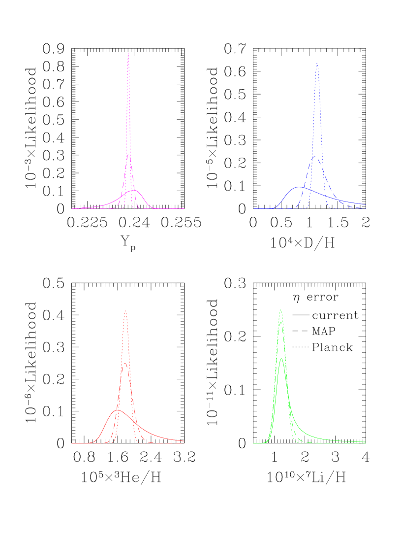
Figure 12: Light element abundances as might be predicted by $\eta$ inputs from future CMB experiments. We have assumed a central value of $\eta_{10}=\hat{\eta}_{10}$ (eq. 19). Solid curve: 10% errors in $\eta$ (MAP); Broken curve: 3% errors in $\eta$ (PLANCK). We see that predictive power of the CMB limits on $\eta$ will become quite strong.

On the other hand, it is possible that, with precision results available for both BBN and the CMB, the baryonic predictions will be in agreement. Then, as the CMB results improve, it will become useful to use the CMB range for $\eta$ as an input to the BBN analysis, and to use this, e.g., to give precision predictions for the light element abundances. An illustration of such a prediction is shown in Figure 12, which shows the light element abundance predictions assuming a constant central value of $\eta_{10}=\hat{\eta}_{10}$ (as in eq. 19), but with an error which goes from that of our current limits down to 10% (MAP) and then 3% (PLANCK). We see that these experiments will be able to determine the primordial abundances quite accurately and thus will impact studies of galactic, stellar, and cosmic-ray evolution.

A noteworthy feature of Figure 12 is the slight shift in the peak values of the likelihoods as the limits on $\eta$ become tighter. Thus, the maximum likelihood estimator for the abundance $y$ is slightly offset from $y_{\rm BBN}(\hat{\eta})$ but converges to this value as the CMB uncertainty in $\eta$ becomes small. This comes about because the plotted likelihood is given by the convolution

$$L(y)=\int d\eta\;L_{\rm CMB}(\eta)\;L_{\rm BBN}(\eta;y)$$ (26)

The BBN theory likelihood

$$L_{\rm BBN}\propto\sigma_{\rm BBN}^{-1}\;\exp[-(y-y_{\rm BBN})^{2}/2\sigma_{\rm BBN}^{2}]$$ (27)

depends on $\eta$ in a complicated way through the abundance and error curves $y_{\rm BBN}(\eta)$ and $\sigma_{\rm BBN}(\eta)$. One can show that the peak of $L(y)$ is shifted due to the variation of the mean values and errors with $\eta$. One can also show that the shift goes to zero as the CMB error becomes small.

7 Conclusions

We have examined the effect of the NACRE thermonuclear reaction rates on BBN. We verify that the central values of the abundance predictions are very similar to those used in previous studies (cf. Hata et al. 1996). We note that the NACRE fits are in general good representations of the shape of the data, but the normalizations do not precisely minimize $\chi^{2}$. We have thus computed the renormalizations needed to minimize $\chi^{2}$. Although small, the renormalizations do lead to changes with the previous predictions, particularly in that the Li prediction at high $\eta$ is reduced, and thus less Li depletion is required in this regime.

We have used the NACRE rates and database to determine the theoretical uncertainty in BBN via the standard Monte Carlo procedure. To do this we have examined the effect of different estimates of the nuclear reaction uncertainties. NACRE’s high/low limits give BBN uncertainties similar to those of SKM. Using a simple sample variance procedure, we arrive at errors which are smaller than these, while being slightly larger than those of Nollett and Burles. We have also computed lower limits to the errors on the reaction rates, which lead to the minimal theoretical errors on the light element abundances.

Error studies such as ours are increasingly important as cosmology enters the precision era. In particular, an independent prediction of $\eta$ is emerging from CMB anisotropy data. At present, the CMB results are tantalizing, and possibly discrepant with the BBN predictions, though the CMB predictions for $\eta$ seem to be uncertain at the moment. At any rate, the CMB data will improve dramatically with the upcoming launch of MAP; this experiment, along with PLANCK, will make a strong test of BBN and of cosmology.

In anticipation of this test, further work is needed to find a realistic error budget for both the theory and observation of light element abundances. A key input on the theory side can come from accurate nuclear experimental data and careful analyses of the error budget in key reactions. Specifically, we urge more data be taken for $p(n,\gamma)d$, in order to confirm theory, and put this reaction on a solid empirical basis. Other key reactions are those with internally discrepant reactions, $d(p,\gamma)\mbox{${}^{3}{\rm He}$}$ and $\mbox{${}^{3}{\rm He}$}(d,p)\mbox{${}^{4}{\rm He}$}$, and the lithium sources and sinks, $t(\alpha,\gamma)\mbox{${}^{7}{\rm Li}$}$, $\mbox{${}^{3}{\rm He}$}(\alpha,\gamma)\mbox{${}^{7}{\rm Be}$}$, and $\mbox{${}^{7}{\rm Li}$}(p,\alpha)\mbox{${}^{4}{\rm He}$}$.

References

- (1) Adelberger, E.G., et al. 1998, Rev. Mod. Phys., 70, 1265
- (2) Angulo, C., et al. 1999, Nucl. Phys. A., 656, 3 (NACRE)
- (3) Arzumanov, S., et al. 2000, Nucl. Inst. Meth. A, 440, 511
- (4) Balbi, et al. 2000, ApJ, 545, L1
- (5) Bonifacio, P. & Molaro, P. 1997, MNRAS, 285, 847
- (6) Burles, S., Nollett, K.M., Truran, J.W., & Turner, M.S. 1999, Phys. Rev. Lett., 81, 4176
- (7) Brune, C., Hahan, K.I., Kavanagh, R.W., & Wrean, P.R., 1999, Phys. Rev. C, 60, 015801
- (8) Brune, C.R., Kavanagh, R.W., & Rolfs, C., 1994, Phys. Rev. C., 50, 2205
- (9) Burles, S., & Tytler, D. 1998a, ApJ 499,699
- (10) Burles, S., & Tytler, D. 1998b, ApJ 507, 732
- (11) Caughlan, G., & Fowler, W.A., 1988, Atomic Data Nucl. Data Tables, 40, 283
- (12) Cayrel, R., Spite, M., Spite, F., Vangioni-Flam, E., Cassé, M., & Audouze, J. 1999, AA, 343, 923
- (13) Coc, A., Vangioni-Flam, E., and Casse, M. 2001, astro-ph/0101286
- (14) de Bernardis, P., et al. 2000, Nature, 404, 995
- (15) Dicus, D.A. et al. 1982, Phys. Rev. D, 26, 2694
- (16) Dodelson, S. & Turner, M.S. 1992, Phys. Rev. D, 46, 3372
- (17) Esposito, S., Mangano, G., Melchiorri, A., Miele, G., & Pisanti, O. 2001, Phys. Rev. D, 63, 043004
- (18) Esposito, S., Mangano, G., Miele, G., & Pisanti, O. 2000a, Nucl. Phys. B, 568, 421
- (19) Esposito, S., Mangano, G., Miele, G., & Pisanti, O. 2000b, J. High Energy Phys., 038, 09
- (20) Fields, B. D., Kainulainen, K., Olive, K. A., & Thomas, D. 1996, New Astron., 1, 77
- (21) Fields, B. D. & Olive, K. A. 1996, Phys Lett, B368, 103
- (22) Fields, B. D. & Olive, K. A. 1998, ApJ, 506, 177
- (23) Fields, B. D. & Olive, K. A. 1999, New Ast, 4, 255
- (24) Fiorentini, G., Lisi, E., Sarkar, S., & Villante, F.L. 1998, Phys Rev, D58, 063506
- (25) Griffiths, Lal, M., & Scarfe, C.D., 1963, Canadian J. Phys., 39, 1397
- (26) Groom, D., et al. (Particle Data Group) 2000, European Physical Journal C, 15, 1 and to appear in the 2001 off-year partial update for the 2002 edition available on the PDG WWW pages (URL: http://pdg.lbl.gov/)
- (27) Hale, G. M., Dodder, D. C., Siciliano, E. R., & Wilson, W. B., 1991, ENDF/B-VI Evaluation, Material 125, Revision 1.
- (28) Hanany, S., et al. 2000, ApJL, submitted (astro-ph/0005123)
- (29) Hata, N., Scherrer, R.J., Steigman, G., Thomas, D., & Walker, T.P. 1996, ApJ, 458, 637
- (30) Heckler, A. 1994, Phys. Rev. D, 49, 611
- (31) Hobbs, L. & Thorburn, J. 1994, ApJ, 428 L25
- (32) Hobbs, L. & Thorburn, J. 1997, ApJ, 491, 772
- (33) Izotov, Y.I. & Thuan, T.X. 1998a, ApJ, 497, 227.
- (34) Izotov, Y.I. & Thuan, T.X. 1998b, ApJ, 500, 188.
- (35) Izotov, Y.I., Thuan, T.X., & Lipovetsky, V.A. 1994 ApJ 435, 647
- (36) Izotov, Y.I., Thuan, T.X., & Lipovetsky, V.A. 1997, ApJS, 108, 1
- (37) Jaffe, A., et al. 2000, Phys. Rev. Lett. submitted (astro-ph/0007333)
- (38) Kajino, T. 1986, Nucl. Phys. A, 460, 559
- (39) Kaplinghat, M., & Turner, M.S. 2001, Phys. Rev. Lett., 86, 385
- (40) Kneller, J.P., Scherrer, R.J., Steigman, G., & Walker, T.P. 2001, (astro-ph/0101386)
- (41) Kernan, P. 1993, Ph.D. thesis, The Ohio State University
- (42) Krauss, L.M. & Kernan, P. 1995 Phys Lett, B347, 347
- (43) Krauss, L.M., & Romanelli, P. 1990, ApJ, 358, 47
- (44) Lemoine, M., Schramm, D.N., Truran, J.W., & Copi, C.J. 1997, ApJ, 478, 554
- (45) Lesgourgues, J., & Peloso, M. 2000, Phys. Rev. D, 62, 081301
- (46) Levshakov, S.A., Kegel, W.H., & Takahara, F. 1998, ApJ, 499, L1
- (47) Levshakov, S.A., Tytler, D., & Burles, S., 1998, astro-ph/9812114
- (48) Linsky, J.L. 1998, Space Sci. Rev., 84, 285
- (49) Lisi, E., Sarkar, S., & Villante, F.L. 1999 Phys Rev, D59, 123520
- (50) Lopez, R., & Turner, M.S. 1999, Phys. Rev. D, 59, 103502
- (51) Nagai, Y., et al. 1997, Phys. Rev. C, 56, 3173
- (52) Nissen, P.E., Asplund, M., Hill, V., & D’Ororico, S. 2000, AA, 357, 49
- (53) Nollett, K.M. & Burles, S. 2000, Phys. Rev. D, 61, 123505
- (54) Olive, K.A. & Skillman, E. 2000, astro-ph/0007081.
- (55) Olive, K. A., Steigman, G. & Walker, T.P. 2000, Phys Rep, 333-334, 389
- (56) Olive, K. A., Steigman, G. & Skillman, E. 1997, ApJ, 483, 788
- (57) Olive, K.A. & Thomas, D. 1999, Astr Part Phys, 11, 403
- (58) O’Meara, J.M. et al. 2000, astro-ph/0011179
- (59) Orito, M., Kajino, T., Mathews, G.J., & Boys, R.N. 2000, ApJ, submitted (astro-ph/0005446)
- (60) Padin, S., et al. 2000, ApJ, submitted (astro-ph/0012211)
- (61) Pagel, B.E.J., Simonson, E.A., Terlevich, R.J. & Edmunds, M. 1992, MNRAS, 255, 325
- (62) Pinsonneault, M.H., Walker, T.P., Steigman, G., & Naranyanan, V.K. 1998, ApJ, 527, 180
- (63) Ryan, S.G., Beers, T.C., Olive, K.A., Fields, B.D., & Norris, J. 2000, ApJ, 530, L57
- (64) Ryan, S.G., Norris, J., & Beers, T.C. 1999, ApJ, 523, 654
- (65) Sahu, M.S., et al. 1999, ApJ, 523, L159
- (66) Sarkar, S. 1996, Rep Prog Phys, 59, 1493
- (67) Schmid, G.J., et al. 1995, Phys. Rev. C, 52, R1732
- (68) Schramm, D.N. & Turner, M.S. 1998, Rev Mod Phys, 70, 303
- (69) Seckel, D., 1993 (hep-ph/9305311)
- (70) Skillman, E., & Kennicutt 1993, ApJ, 411, 655
- (71) Skillman, E., Terlevich, R.J., Kennicutt, R.C., Garnett, D.R., & Terlevich, E. 1994, ApJ, 431, 172
- (72) Smith, M.S., Kawano, L.H. & Malaney, R.A. 1993, ApJS, 85, 219 (SKM)
- (73) Smith, V.V., Lambert, D.L., & Nissen, P.E. 1992, ApJ, 408, 262
- (74) Smith, V.V., Lambert, D.L., & Nissen, P.E. 1998, ApJ, 506, 405
- (75) Spite, F. & Spite, M. 1982, A&A, 115, 357
- (76) Steigman, G., Fields, B.D., Olive, K.A., Schramm, D.N., & Walker, T.P. 1993 ApJ, 415 L35
- (77) Suzuki, T.S. et al. 1995, ApJ, 439, L59
- (78) Tegmark, M., Zaldarriaga, M., & Hamilton, A., 2000, Phys. Rev. D, in press (astro-ph/0008167)
- (79) Tegmark, M., Zaldarriaga, M. 2000, Phys. Rev. Lett., 85, 2240
- (80) Thomas, D., Schramm, D.N., Olive, K.A., & Fields, B.D. 1993, ApJ, 406, 569
- (81) Tytler, D., et al. 1999, AJ, 117, 63
- (82) Vangioni-Flam, E., Cassé, M., Cayrel, R., Audouze, J., Spite, M., & Spite, F. 1999, New Ast, 4, 245
- (83) Vangioni-Flam, E., Coc, A., & Cassé, M. 2000, A&A, 360, 15
- (84) Vangioni-Flam, E., Coc, A., & Cassé, M. 2001, in preparation
- (85) Vauclair, S., & Charbonnel, C. 1998, ApJ, 502, 372
- (86) Walker, T.P., Steigman, G., Schramm, D.N., Olive, K.A., & Kang, K. 1991, ApJ, 376, 51
- (87) Webb, J.K., et al. 1997, Nature, 388, 250
- (88) White, M., Scott, D., & Silk, J. 1994, ARAA, 32, 319
- (89) Wright, E.L., 1999, New Astron. Rev., 43, 257