Cluster physics from joint weak gravitational lensing and Sunyaev-Zel’dovich data

We present a self consistent method to perfom a joint analysis of Sunyaev-Zel’dovich and weak gravitational lensing observation of galaxy clusters. The spatial distribution of the cluster main constituents is described by a perturbative approach. Assuming the hydrostatic equilibrium and the equation of state, we are able to deduce, from observations, maps of projected gas density and gas temperature. The method then naturally entails an X-ray emissivity prediction which can be compared to observed X-ray emissivity maps. When tested on simulated clusters (noise free), this prediction turns out to be in very good agreement with the simulated surface brightness. The simulated and predicted surface brightness images have a correlation coefficient higher than $0.9$ and the total flux differ by $0.9\%$ or $9\%$ in the two simulated clusters we studied. The method should be easily used on real data in order to provide a physical description of the cluster physics and of its constituents. The tests performed show that we can recover the amount and the spatial distributions of both the baryonic and non-baryonic material with an accuracy better than 10%. So, in principle, in it might indeed help to alleviate some well known bias affecting, e.g. baryon fraction measurements.

1 Introduction

Whereas clusters of galaxies, as the largest gravitationnaly bound structures of the universe, form natural probe of cosmology, observations, numerical simulations as well as timing arguments provide compelling evidences that most of them are young and complex systems. Interaction with large-scale structures, merging processes and coupling of dark matter with the intra-cluster medium complicate the interpretation of observations and the modeling of each of its components. Since they are composed of dark mater (DM), galaxies and a hot dilute X-ray emitting gas (Intra cluster medium, ICM) accounting respectively for $\sim 85\%$, $\sim 15\%$ and $\sim 5\%$ of their mass, the physics of the ICM bounded in a dark matter gravitational potential plays a major role in cluster formation and evolution. This variety of components can be observed in many various ways. In particular, gravitational lensing effects (the weak-lensing regime here, WL) Mellier (2000); Bartelmann and Schneider (2001), Sunyaev-Zel’dovich (SZ) effect Sunyaev and Zel’dovich (1972); Birkinshaw (1999) and X-ray emission (X) Sarrazin (1988). Whereas the former probes mostly the dark matter component, both the latter probe the baryons of the gravitationally bound ICM.

Due to observational progress, increasingly high quality data are delivered which enables multi-wavelength investigation of clusters on arcminute scale (the most recent is the spectacular progress in SZ measurements, e.g. Reese et al. (2000); Désert et al. (1998)) and we therefore think it is timely to explore how we should perform some joint analysis of these high quality data sets and exploit them at best their complementarity. This challenge has already been tackled by several groups Zaroubi et al. (1998); Grego et al. (1999); Reblinsky (2000); Zaroubi et al. (2000); Castander et al. (2000); Holder et al. (2000). Zaroubi et al. and Reblinsky et al. attempted a full deprojection by assuming isothermality and axial symmetry, using respectively a least square minimization or a Lucy-Richardson algorithm , Grego et al. compare SZ derived gas mass to WL derived total mass by fitting a spheroidal $\beta$ model. But whereas these methods give reasonable results it has been illustrated, e.g. by Inagaki et al. 1995 in the context of $H_{0}$ measurement from SZ and X-ray observations, that both non isothermality and asphericity analysis can trigger systematic errors as high as $20\ \%$. Therefore, we aim at exploring an original approach which allows to get rid of both isothermality and departure from sphericity. Based on a self-consistent use of both observables, and based on a perturbative development of general physical hypothesis, this method allow us to test some very general physical hypothesis of the gas (hydrostatic equilibrium, global thermodynamic equilibrium) and also provide naturally some X observation predictions.

Observations only provide us with $2-D$ projected quantities (e.g. mass, gas pression,…). This quantities are related by some physical hypothesis which are explicited in $3-D$ equalities (e.g. hydrostatic equilibrium, equation of state). The point is that these $3-D$ equalities do not have any tractable equivalent relating projected $2-D$ quantities: in particular, projection along the line of sight does not provide an equation of state or a projected hydrostatic equilibrium equation. Therefore as soon as we want to compare this data (WL, SZ, X) we have to deproject the relevant physical quantities ($P_{g},T_{g},\rho_{g}$…). This can be done only using strong assumptions, either by using parametric models (e.g. a $\beta$ model Cavaliere & Fusco-Femaino (1976)) or by assuming mere geometrical hypothesis (the former necessarily encompassing the latter) Fabian et al. (1981); Yoshikawa and Suto (1999). We choose the geometric approach in order to use as general physical grounds as possible and to avoid as many theoretical biases as possible.

This simplest choice might be naturally motivated first by looking at some images of observed clusters Désert et al. (1998); Grego et al. (1999). Their regularity is striking : some have almost circular or ellipsoidal appearance as we expect for fully relaxed system. Then since relaxed clusters are expected to be spheroidal in favored hierarchical structure formation scenario, it is natural to try to relate the observed quasi-circularity (quasi-sphericity) to the $3-D$ quasi-sphericity (quasi-spheroidality). We perform this using some linearly perturbed spherical (spheroidal) symmetries in a self-consistent approach.

We proceed as follows: in section 2 we defined our physical hypothesis and our notations. The method is precisely described in section 3. We consider both the spherical as well as spheroidal cases and obtain a predicted X surface brightness map from a SZ decrement map and a WL gravitational distortion map. In section 4 a demonstration with simulated clusters is presented before discussing its application to genuine data as well as further developments in section 5.

2 Hypothesis, Sunyaev-Zel’dovich effect and the Weak lensing

We now briefly describe our notations as well as our physical hypothesis.

2.1 General hypothesis

Following considerations fully detailed in Sarrazin (1988) the ICM can be regarded as a hot and dilute plasma constituted from ions and electrons, whose respective kinetic temperatures $T_{p}$ and $T_{e}$ will be considered as equal $T_{p}=T_{e}\equiv T_{g}$. This is the global thermodynamic equilibrium hypothesis which is expected to hold up to $r_{virial}$ ( see Teyssier et al. (1997); Chièze et al. (1998) for a precise discussion). Given the low density (from $n_{e}\sim 10^{-1}\rm{cm^{-3}}$ in the core to $\sim 10^{-5}\rm{cm^{-3}}$ in the outer part) and high temperature of this plasma ($\sim 10\rm{keV}$), it can be treated as a perfect gas satisfying the equation of state :

$$P_{g}\ =\ \frac{\rho_{g}\ k_{B}\ T_{g}}{\mu_{e}\ m_{p}}\ =\ \beta\ \rho_{g}T_{g}$$ (1)

with $\beta\equiv\frac{\ k_{B}}{\mu_{e}\ m_{p}}$. Let us neglect then the gas mass with regards to the dark matter mass, and assume stationarity (no gravitational potential variation on time scale smaller than the hydrodynamic time scale, e.g. no recent mergers). Then the gas assumed to be in hydrostatic equilibrium in the dark matter gravitational potential satisfies:

$$\nabla(\rho_{g}\mathbf{v_{g}}) = 0$$ (2)

$$\nabla P_{g} = -\rho_{g}\nabla\Phi_{DM}\>.$$ (3)

At this point there is no need to assume isothermality.

2.2 Sunyaev-Zel’dovich effect and weak lensing

Inverse Compton scattering of cosmic background (CMB) photons by the electrons in the ICM modifies the CMB spectrum Zel’dovich and Sunyaev (1969); Sunyaev and Zel’dovich (1972, 1980). The amplitude of the SZ temperature decrement $\Delta T_{SZ}\over T_{CMB}$ is directly proportional to the Comptonisation parameter $y$ which is given by :

$$y\ =\ \frac{\sigma_{T}}{m_{e}c^{2}}\int dl\ n_{e}k_{B}T_{e}\ = \ \frac{\sigma_{T}}{m_{e}c^{2}}\int dl\ p_{e}$$ (4)

$$=\ \frac{\sigma_{T}}{m_{e}c^{2}}\int dl\frac{\rho_{g}k_{B}T_{g}}{\mu_{e}m_{p}}\ = \ \alpha\int dlP_{g}\>.$$ (5)

where $\alpha\equiv\frac{\sigma_{T}}{m_{e}c^{2}}$, $k_{B}$ is the Boltzmann’s constant, $\sigma_{T}$ is the Thomson scattering cross section and $dl$ is the physical line-of-sight distance. $m_{e}$, $n_{e}$, $T_{e}$ and $p_{e}$ are the mass, the number density, the temperature and the thermal pressure of electrons. $\rho_{g}$ and $T_{g}$ respectively denote the gas density and temperature, and $\mu_{e}$ is the number of electrons per proton mass. Some further corrections to this expression can be found in Rephaeli (1995); Birkinshaw (1999).

In parallel to this spectral distortions, the statistical determination of the shear field $\kappa$ affecting the images of background galaxies enable, in the weak lensing regime, to derive the dominant projected gravitational potential of the lens (the clustered dark matter) : $\phi_{DM}$ in our general hypothesis (see Mellier (2000) for details).

3 Method

3.1 Principle

We now answer the question : how should we co-analyze these various data set ? Our first aim is to develop a method which allows us to get maps of projected thermodynamical quantities with as few physical hypothesis as possible.

Our method is the following. Let us suppose we have for a given cluster a set of data a SZ and WL data which enables us to construct a $2-D$ map of projected gas pressure as well as a $2-D$ projected gravitational potential map. Let us suppose as well that these maps exhibit an approximate spherical symmetry as it is the case for a vast class of experimental observations as e.g. in figure 1. More precisely, let us suppose that the projected gas pressure $y$ as well as the observed projected gravitational potential $\phi_{DM}$ can be well fitted by the following type of functions :

$$y(R,\varphi) = y_{0}(R)+\varepsilon y_{1}(R)\ m(\varphi)$$ (6)

$$\phi_{DM}(R,\varphi) = \phi_{DM,0}(R)+\varepsilon\phi_{DM,1}(R)\ n(\varphi)$$ (7)

where $\varepsilon\ll 1$, $(R,\varphi)$ denotes polar coordinates in the image plane and $m$ and $n$ are some particular functions. This description means first of all that the images we see are linear perturbations from some perfect circularly symmetric images, and second that the perturbation might be described conveniently by the product of a radial function and an angular function. Equivalently we can assert that to first order in $\varepsilon$ our images are circularly symmetric but they admit some corrections to second order in $\varepsilon$.
We then assume that these observed perturbed symmetries are a consequence of an intrinsic $3-D$ spherical symmetry linearly perturbed too. This point constitutes our key hypothesis. It means that to first order in a certain parameter (e.g. $\varepsilon$) our clusters are regular objects with a strong circular symmetry but they admit some second order linear perturbations away from this symmetry. As a consequence of these assumptions we will make use of this linearly perturbed symmetry to get a map of some complementary projected thermodynamical quantities, the gas density $D_{g}$ and the gas temperature $\zeta_{g}$, successively to first and second order in $\varepsilon$.

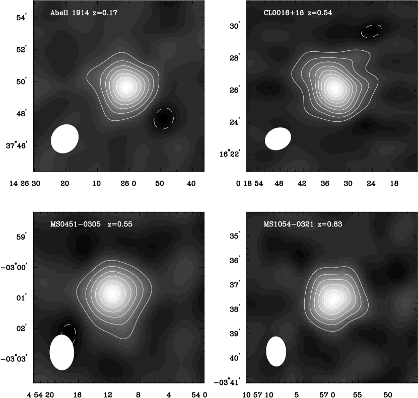
Figure 1: Images of the SZ effect observed towards four galaxy clusters with various redshifts. The contours correspond to 1.5 to 5 times the noise level. Data taken with the low-noise cm-wave receiver installed on the OVRO and BIMA mm-wave interferometric arrays (Holder and Carlstrom 1999).

Formulated this way, the problem yields a natural protocol :

• Looking at some maps with this kind of symmetry, we compute a zero-order map ($y_{0}(R)$, $\phi_{0}(R)$) with a perfect circular symmetry by averaging over some concentric annulus. A correction for the bias introduced by perturbations is included. These first order quantities allow us to derive some first order maps of $D_{g,0}(R)$ and $\zeta_{g,0}(R)$ with a perfect circular symmetry.

• We then take into account the first order corrections to this perfect symmetry ($y_{1}(R)m(\varphi)$, $\phi_{1}(R)m(\varphi)$) and infer from them first order correction terms to the zeroth order maps: $D_{g,1}(R,\varphi)$ and $\zeta_{g,1}(R,\varphi)$.

Even if for clarity’s sake we formulate our method assuming a perturbed circular symmetry, it applies equivalently to a perturbed elliptical symmetry as it will be shown below. In this more general case, we assume that the cluster exhibit a linearly perturbed spheroidal symmetry.

3.2 The spherically symmetric case : from observations to predictions

Let us now apply the method to the case where the projected gas density (SZ data) and the projected gravitational potential (WL data) exhibit some approximate circular symmetry. These observations lead us to suppose that the $3-D$ gas pressure, the gravitational potential, the gas density and the gas temperature can be well described by the following equations:

$$\left\{\begin{array}[]{cccccc}P_{g}(r,\theta,\varphi)&=&P_{g,0}(r)&+&\varepsilon&P_{g,1}(r)f(\theta,\varphi)\\ \Phi_{DM}(r,\theta,\varphi)&=&\Phi_{DM,0}(r)&+&\varepsilon&\Phi_{DM,1}(r)g(\theta,\varphi)\\ \rho_{g}(r,\theta,\varphi)&=&\rho_{g,0}(r)&+&\varepsilon&\rho_{g,1}(r)h(\theta,\varphi)\\ T_{g}(r,\theta,\varphi)&=&T_{g,0}(r)&+&\varepsilon&T_{g,1}(r)k(\theta,\varphi)\end{array}\right.$$ (8)

where $(r,\theta,\varphi)$ are spherical coordinates centered on the cluster.

3.2.1 The hydrostatic equilibrium

If we first apply the hydrostatic equilibrium equation $\nabla P_{g}=-\rho_{g}\nabla\Phi_{DM}$ we get the following equations. To first order in $\varepsilon$ we have

$$P^{\prime}_{g,0}(r)\ =\ -\rho_{g,0}(r)\Phi^{\prime}_{DM,0}(r)\>,$$ (9)

and to second order in $\varepsilon$ :

$$\left\{\begin{array}[]{cccc}P^{\prime}_{g,1}(r)f(\theta,\varphi)&=&\ -\rho_{g,0}(r)\Phi^{\prime}_{DM,1}(r)\ h(\theta,\varphi)&\\ &&-\rho_{g,1}(r)\Phi^{\prime}_{DM,0}(r)\ g(\theta,\varphi)&\>(a)\\ P_{g,1}(r)\ \partial_{\theta}\ f(\theta,\varphi)&=&\ -\rho_{g,0}(r)\ \Phi_{DM,1}(r)\ \partial_{\theta}h(\theta,\varphi)&\>(b)\\ P_{g,1}(r)\ \partial_{\varphi}f(\theta,\varphi)&=&\ -\rho_{g,0}(r)\ \Phi_{DM,1}(r)\ \partial_{\varphi}h(\theta,\varphi)&\>(c)\end{array}\right.$$ (10)

where   “ ’ “  denotes the derivative with regards to $r$.
Combining equations (10.b) and (10.c) we get

$$f(\theta,\varphi)=\lambda_{1}h(\theta,\varphi)+\lambda_{2}$$ (11)

where $\lambda_{1,2}$ are some constants. Then, using equation (10.a) we can write

$$f(\theta,\varphi)=\gamma_{1}g(\theta,\varphi)+\gamma_{2}$$ (12)

where $\gamma_{1,2}$ are some constants as well. At this point, we can get rid of $\lambda_{2}$ and $\gamma_{2}$ by absorbing them in the order $1$ mere radial term (i.e. $\rho_{g,0}(r)$ and $\Phi_{DM,0}(r)$). This means we can consider $\lambda_{2}=0$ and $\gamma_{2}=0$ . Similarly we choose to rescale $\rho_{g,1}(r)$ and $\Phi_{DM,1}(r)$ so that we can take $\gamma_{1}=\lambda_{1}=1\$. These simple equalities lead us to assume from now on :

$$f(\theta,\varphi)=h(\theta,\varphi)=g(\theta,\varphi)\>.$$ (13)

This is in no way a restriction since it simply means that we absorb integration constants by redefining some terms. This is possible since the relevant part of $f$ (and thus $h$) will be fitted on observations as will be shown below. Taking equation (13) into account, equation (10) simplifies to :

$$P^{\prime}_{g,0}(r)\ = \ -\rho_{g,0}(r)\Phi^{\prime}_{DM,0}(r)$$ (14)

$$P^{\prime}_{g,1}(r)\ = \ -\rho_{g,0}(r)\Phi^{\prime}_{DM,1}(r)-\rho_{g,1}(r)\Phi^{\prime}_{DM,0}(r)$$ (15)

$$P_{g,1}(r)\ = \ -\rho_{g,0}(r)\Phi_{DM,1}(r)\>.$$ (16)

3.2.2 The equation of state

We have now identified the angular part to the first order correction of $P_{g}$, $\Phi_{DM}$ and $\rho_{g}$. We still have to link those quantities to the angular dependent part of the temperature $T_{g}$, namely $k(\theta,\varphi)$. This is done naturally using the equation of state (1), which directly provide to first and second order in $\varepsilon$ :

$$P_{g,0}(r)\ = \ \beta\rho_{g,0}(r)T_{g,0}(r)$$ (17)

$$P_{g,1}(r)f(\theta,\varphi)\ = \ \beta\rho_{g,1}(r)T_{g,0}(r)f(\theta,\varphi)$$

$$+ \beta\rho_{g,0}(r)T_{g,1}(r)k(\theta,\varphi)$$ (18)

This last equation leads naturally to $f(\theta,\varphi)=k(\theta,\varphi)$ if we decide once again to absorb any multiplicative factor in the radial part. This way we see that our choice of separating the radial and angular part is in no way a restriction. We eventually get

$$P_{g,0}(r)\ = \ \beta\rho_{g,0}(r)T_{g,0}(r)$$ (19)

$$P_{g,1}(r)\ = \ \beta\rho_{g,1}(r)T_{g,0}(r)+\beta\rho_{g,0}(r)T_{g,1}(r)\>.$$ (20)

3.2.3 The observations

Given this description of the cluster hot gas, the experimental SZ and WL data which respectively provide us with the projected quantities $y(R,\varphi)$ and $\phi_{DM}(R,\varphi)$ write

$$y(R,\varphi) = \alpha\int P_{g,0}(r)dl+\varepsilon\ \alpha\int P_{g,1}(r)f(\theta,\varphi)dl\$$ (21)

$$\equiv \ y_{0}(R)+\varepsilon y_{1}(R)m(\varphi)$$

$$\phi_{DM}(R,\varphi) = \int\Phi_{DM,0}(r)dl+\varepsilon\int\Phi_{DM,1}(r)f(\theta,\varphi)dl\$$ (22)

$$\equiv \ \phi_{DM,0}(R)+\varepsilon\phi_{DM,1}(R)m(\varphi)\>.$$

Note that in order to get this set of definitions we choose the polar axis of the cluster along the line of sight so that the same azimuthal angle $\varphi$ is used for $2-D$ and $3-D$ quantities.

Our aim is now to derive both a projected gas density map and projected temperature map that we define this way :

$$D_{g}(R,\varphi) = \int\ \rho_{g}(r,\varphi)dl$$ (23)

$$= \int\rho_{g,0}(r)dl+\varepsilon\int\rho_{g,1}(r)f(\theta,\varphi)dl$$ (24)

$$\equiv \ D_{g,0}(R)+D_{g,1}(R,\varphi)$$ (25)

$$\zeta_{g}(R,\varphi) = \int\ T_{g}(r,\varphi)dl$$ (26)

$$= \int\ T_{g,0}(r)\ dl+\varepsilon\int\ T_{g,1}(r)f(\theta,\varphi)dl$$ (27)

$$\equiv \zeta_{g,0}(R)+\zeta_{g,1}(R,\varphi)\>.$$ (28)

3.2.4 A projected gas density map to first order…

Now that we have expressed our observables in terms of $3-D$ physical quantities, it is easy to infer a gas density map successively to first and second order in $\varepsilon$. To first order the hydrostatic equilibrium condition (9) states that

$$P^{\prime}_{g,0}(r)\ =\ -\rho_{g,0}(r)\Phi^{\prime}_{DM,0}(r)\>.$$ (29)

In order to use it we need to deproject the relevant quantities. From the well known spherical deprojection formula Binney and Tremaine (1987) based on Abel’s transform we have :

$$\alpha\ P_{g,0}(r) = -{1\over\pi}\int_{r}^{\infty}y^{\prime}_{0}(R){dR\over(R^{2}-r^{2})^{1\over 2}}$$ (30)

$$= -{1\over\pi}\int_{0}^{\infty}\ y^{\prime}_{0}(r\cosh u)du$$ (31)

where $R=r\cosh u$. Thus, we can write

$$\alpha\ P^{\prime}_{g,0}(r) = -{1\over\pi}\int_{0}^{\infty}\ \cosh u\ y^{\prime\prime}(r\cosh u)du$$ (32)

$$= -{1\over\pi}\int_{r}^{\infty}\ {1\over r}{R\over(R^{2}-r^{2})^{1\over 2}}\ y^{\prime\prime}_{0}(R)dR\;.$$ (33)

Similarly,

$$\Phi^{\prime}_{DM,0}(r)=-{1\over\pi}\int_{r}^{\infty}\ {1\over r}{R\over(R^{2}-r^{2})^{1\over 2}}\ \phi_{0}^{\prime\prime}(R)dR\;.$$ (34)

We then get for the projected gas density

$$D_{g,0}(R)=-2\int_{R}^{\infty}{rdr\over(r^{2}-R^{2})^{1\over 2}}{P^{\prime}_{g,0}(r)\over\Phi^{\prime}_{DM,0}(r)}$$ (36)

$$=-{2\over\alpha}\int_{R}^{\infty}{rdr\over(r^{2}-R^{2})^{1\over 2}}\left(\frac{\int_{r}^{\infty}{s\ ds\over r(s^{2}-r^{2})^{1\over 2}}\ y^{\prime\prime}_{0}(s)}{\int_{r}^{\infty}{s\ ds\over r(s^{2}-r^{2})^{1\over 2}}\ \phi^{\prime\prime}_{0}(s)}\right)\>.$$

3.2.5 …and a projected gas temperature map to first order

Once we built this projected gas density map, we can recover the projected gas temperature map. If we apply the equation of state (17) we get :

$$\zeta_{g,0}(R) = {1\over\beta}\int{P_{g,0}(r)\over\rho_{g,0}(r)}dl$$ (37)

$$= -{1\over\beta}\int{P_{g,0}(r)\over P^{\prime}_{g,0}(r)}\Phi^{\prime}_{DM,0}(r)dl$$ (38)

$$= -{1\over\pi\beta}\int_{R}^{\infty}\ {P_{g,0}(r)\over P^{\prime}_{g,0}(r)}\Phi^{\prime}_{DM,0}(r){rdr\over(r^{2}-R^{2})^{1\over 2}}\>.$$ (39)

Since all the required functions ($P_{g,0}$, $P^{\prime}_{g,0}$, $\Phi^{\prime}_{DM,0}$) have been derived in the previous section (equation (31) and (33)) we can get this way a projected gas temperature map.

3.2.6 Corrections from departure to spherical symmetry : a projected gas density map to second order…

We now reach the core of our method, namely we aim at deriving the quantity $D_{g,1}$ defined by (25), i.e. the second order correction to the perfectly circular term :

$$D_{g}(R,\varphi) = \ D_{g,0}(R)+\varepsilon D_{g,1}(R,\varphi)$$ (40)

$$= \int\rho_{g,0}(r)dl+\varepsilon\int\rho_{g,1}(r)f(\theta,\varphi)dl\>.$$ (41)

If we derive equation (16) and combine it with equation (15) we note that

$$\rho^{\prime}_{g,0}(r)\Phi_{DM,1}(r)\ = \ \rho_{g,1}(r)\Phi^{\prime}_{DM,0}(r)\>.$$ (42)

Therefore we can write

$$\int\rho_{g,1}(r)f(\theta,\varphi)dl=\int\ \frac{\rho^{\prime}_{g,0}(r)}{\Phi^{\prime}_{DM,0}(r)}\ \Phi_{DM,1}(r)f(\theta,\varphi)dl\>.$$ (43)

At this point we want to express this quantity either in terms of WL data or in terms of SZ data depending on the quality of them, or even better in terms of an optimal combination of them.

On one hand, WL data provide us with a straightforward access to the function $\phi_{1}(R)m(\varphi)\ =\ \int\Phi_{DM,1}(r)f(\theta,\varphi)dl$ thus we choose to approximate (43) by

$$\int\rho_{g,1}(r)f(\theta,\varphi)dl\simeq\frac{\rho^{\prime}_{g,0}(R)}{\Phi^{\prime}_{DM,0}(R)}\int\Phi_{DM,1}(r)f(\theta,\varphi)dl$$ (44)

$$\>\simeq\frac{\rho^{\prime}_{g,0}(R)}{\Phi^{\prime}_{DM,0}(R)}\phi_{1}(R)m(\varphi)$$

$$\>\simeq\frac{\rho^{\prime}_{g,0}(R)}{\Phi^{\prime}_{DM,0}(R)}\left(\phi_{DM}(R,\varphi)-\phi_{0}(R)\right)$$

where we used the definitions of section (3.2.3) and where $R$ corresponds to the radius observed in the image plane, i.e. the radius $r$ equal to the distance between the line of sight and the center of the cluster. We will discuss this approximation in more details in section (3.2.8) and validate it through a practical implementation on simulations in section (4). But we already can make the following statements: would the line of sight follows a line of constant $r$ throughout the domain of the perturbation, this expression would be rigorously exact. Moreover it turns out to be a good approximation because of the finite extent of the perturbation.

On the other hand SZ data provide us with a measurement of the function $y_{1}(R)m(\varphi)\ =\ \int P_{g,1}(r)f(\theta,\varphi)dl$ therefore we can use equation (16) and (14) to write

$$\int\rho_{g,1}(r)f(\theta,\varphi)dl=\int\frac{\rho^{\prime}_{g,0}(r)}{P^{\prime}_{g,0}(r)}\ P_{g,1}(r)f(\theta,\varphi)dl$$ (45)

$$\simeq \frac{\rho^{\prime}_{g,0}(R)}{P^{\prime}_{g,0}(R)}\int P_{g,1}(r)f(\theta,\varphi)dl$$ (46)

$$\simeq \frac{\rho^{\prime}_{g,0}(R)}{P^{\prime}_{g,0}(R)}y_{1}(R)m(\varphi)$$ (47)

$$\simeq \frac{\rho^{\prime}_{g,0}(R)}{P^{\prime}_{g,0}(R)}\left(y(R,\varphi)-y_{0}(R)\right)\ .$$ (48)

Here again we used the same notation and approximation as in equation (44). Note however that as soon as we assumed isothermality, the ratio $\rho^{\prime}_{g,0}/P^{\prime}_{g,0}\displaystyle$ is constant therefore this last step is exact. Were we not assuming isothermality, the departure from isothermality is expected to be weak thus this last approximation should be reasonable.

This last two alternative steps are crucial to our method since these approximations link the non spherically symmetric components of various quantities. They are reasonable as will be discussed in section (3.2.8) and will be numerically tested in section (4).
Of course, only well-known quantities appear in equation (44) and (48): $y$, $y_{0}$, $\phi_{DM}$ and $\phi_{0}$ are direct observational data whereas $P_{g,0}(r)$ and $\rho_{g,0}(r)$ are zeroth order quantities previously derived.

3.2.7 …and a projected gas temperature map to second order

The projected temperature map can be obtained the same way as before. Using first the equation of state we can write :

$$T_{g,0}(r)+\varepsilon T_{g,1}(r)f(\theta,\varphi)={1\over\beta}{(P_{g,0}(r)+\varepsilon P_{g,1}(r)f(\theta,\varphi))\over(\rho_{g,0}(r)+\varepsilon\rho_{g,1}(r)f(\theta,\varphi))}$$ (49)

$$\simeq {1\over\beta}\left({P_{g,0}(r)\over\rho_{g,0}(r)}+\varepsilon P_{g,1}(r){\rho_{g,0}(r)-\rho_{g,1}(r)\over\rho^{2}_{g,0}(r)}f(\theta,\varphi)\right)\;.$$

Hence, since

$$\zeta(R,\varphi) = \ \zeta_{0}(R,\varphi)+\varepsilon\zeta_{1}(R,\varphi)$$ (50)

$$= \ \int T_{g,0}(r)\ dl+\varepsilon\int T_{g,1}(r)f(\theta,\varphi)dl$$ (51)

we have

$$\zeta_{1}(R,\varphi)=\int{\rho_{g,0}(r)-\rho_{g,1}(r)\over\rho^{2}_{g,0}(r)}\ P_{g,1}(r)f(\theta,\varphi)dl\>.$$ (52)

Here we choose to approximate the last integral as previously discussed in order to make use of observational SZ data. Therefore we rewrite this last equation as :

$$\zeta_{1}(R,\varphi)\simeq{\rho_{g,0}(R)-\rho_{g,1}(R)\over\rho^{2}_{g,0}(R)}\ \int P_{g,1}(r)f(\theta,\varphi)dl$$ (53)

$$\simeq {\rho_{g,0}(R)-\rho_{g,1}(R)\over\rho^{2}_{g,0}(R)}\ y_{1}(R)m(\varphi)$$

$$\simeq {\rho_{g,0}(R)-\rho_{g,1}(R)\over\rho^{2}_{g,0}(R)}\left(y(R,\varphi)-y_{0}(R)\right)\>.$$ (54)

We obtain this way an expression to second order for the projected temperature in terms of either observed quantities or previously derived functions.

3.2.8 Why the previous approximation is reasonable on intuitive grounds?

Our previous approximations can be justified on intuitive grounds even if we will take care of validating it numerically in section (4) below. It relies on the fact that perturbations have by definition a finite extent, i.e. the first order correction to the perfectly circular (spherical) term is non zero only within a finite range. The typical size and the amplitude of the perturbation can be easily scaled from the SZ and WL data set. This guarantees the validity of our assumptions on observational grounds. The key point is that the perturbation itself has a kind of axial symmetry, whose axis goes through the center of the cluster and the peak of the perturbation. This is reasonable if the perturbation originates in e.g. an incoming filament but not for a substructure. The latter would therefore have to be treated separately by superposition (see section (5)). This leads naturally to the statement that the typical angle we observe in the image plane is equal to the one we would observe if the line of sight were perpendicular to its actual direction, i.e. the perturbation as intrinsically the same angular extent in the directions along the line of sight and perpendicular to it. This is illustrated schematically in figure (2).

Figure 2: We represent schematically in (a) an image corresponding to our hypothesis. The full line corresponds to the perfectly circular $2-D$ term, e.g. $\phi_{DM,0}$, and the dashed line to the first perturbative correction to it, e.g. $\phi_{DM,1}m(\varphi)$, $\Delta\varphi$ represents the observed angular extent. In (b) we represent a schematic slice in the $3-D$ potential responsible for this image. This slice has been performed along the dash-two-dotted plane indicated on figure (a). Here again, the full line corresponds to the perfectly circular $3-D$ term, e.g. $\Phi_{DM,0}$, and the dashed line to the first perturbative correction to it, e.g. $\Phi_{DM,1}f(\theta,\varphi)$. The line of sight direction is indicated by the full thin line. Were the line of sight perpendicular to this slice plane, we would observe the angular extent $\Delta\theta$. Giving an axial symmetry to this perturbation leads us to assess that $\Delta\varphi\simeq\Delta\theta$.

Given this description we are now in a position to discuss the validity of our approximation. It consists in approximating the line of sight integral $\int g(r)\Phi_{DM,1}(r)f(\theta,\varphi)dl\displaystyle$ by $g(R)\int\Phi_{DM,1}(r)f(\theta,\varphi)dl\displaystyle$ where $g$ is any radial function. This approximation would be exact if $g(r)$ were constant in the relevant domain, i.e. if the line of sight had a constant $r$. As mentioned before this is the case in equation 48 if we assume isothermality. But the functions $g(r)$ we might deal with may scale roughly as $r^{2}$, as e.g. $\rho^{\prime}_{g,0}(r)/P_{g,0}(r)$ in equation (44), thus it is far from being constant. The consequent error committed can be estimated by the quantity $\Delta rg^{\prime}(r)$ where $\Delta r$ is the maximum $r$ discrepancy between the value assumed, $g(R)$, and the actual value as it is schematically illustrated in figure (3). In the worst case, $g^{\prime}(r)$ scales as $r$. Then, using the obvious notations defined in this figure we get

$$(\Delta r)_{max}=R(1-1/\sin(\theta-{\Delta\theta\over 2}))\>.$$ (55)

Naturally this quantity is minimal for $\theta\simeq 90^{o}$ and diverges for $\theta\simeq 0^{o}$ when $\Delta\theta=0^{o}$ : the error is minimal when the line of sight is nearly tangential ($\theta\simeq 90^{o}$) and so almost radial in this domain, and maximal when it is radial ($\theta=0^{o}$). This in principle is a very bad behavior, but the fact is that the closer $\theta$ is from $0^{o}$ the weaker the integrated perturbation is since it gets always more degenerate along the line of sight, i.e. the integrated perturbations tend to a radial behavior and will therefore be absorbed in the $\Phi_{DM,0}(r)$ term. The extreme situation, i.e. when $\theta=0^{o}$ will trigger a mere radial image as long as the perturbation exhibits a kind of axial symmetry. This error is impossible to alleviate since we are dealing with a fully degenerate situation but will not flaw the method at all since the integrated perturbation will be null. This approximation will be validated numerically below.

Figure 3: We define in this figure the notation necessary to discuss our approximation. $r_{R}$ is the parameter value given to the function $(f(r))_{R}$ and $r_{R}+\Delta r$ is an actual value along the line of sight.

3.3 How to obtain a X prediction ?

The previously derived map offers a great interest that we now aim at exploiting, namely the ability of precise X prediction. Indeed, for a given X spectral emissivity model, the X-ray spectral surface brightness is

$$S_{X}(E)={1\over 4\pi(1+z)^{4}}\int\ n_{e}^{2}\Lambda(E,T_{e})\ dl$$ (56)

where $\Lambda$ is the spectral emissivity, $z$ is the redshift of the cluster and $E$ is the energy on which the observed band is centered. Hence we can write, assuming a satisfying knowledge of $z$ and $\Lambda$ :

$$S_{X}(E) \propto \int\ n_{e}^{2}T_{e}^{1/2}\ dl$$ (57)

$$\propto \int\ \rho_{g}^{2}T_{g}^{1/2}\ dl$$ (59)

$$\propto \int\ \rho_{g,0}^{2}T_{g,0}^{1/2}\ dl+2\ \varepsilon\int\ \rho_{g,0}T_{g,0}^{1/2}\rho_{g,1}f(\theta,\varphi)dl$$

$$+\>\>\>{1\over 2}\ \varepsilon\int\ \rho_{g,0}^{2}T_{g,0}^{-1/2}T_{g,1}f(\theta,\varphi)dl$$

where we omitted to write the $(r)$s for clarity’s sake. If we now make use of the same approximation as used and discussed before, we can express directly this quantity in terms of observations $y$ and $\phi$. We get indeed

$$S_{X}(E) \propto \int\rho_{g,0}^{2}T_{g,0}^{1/2}dl$$ (61)

$$+\>\>\>2\ \varepsilon\ \rho_{g,0}(R)T_{g,0}^{1/2}(R)\int\rho_{g,1}f(\theta,\varphi)dl$$

$$+\>\>\>{1\over 2}\ \varepsilon\ \rho_{g,0}^{2}(R)T_{g,0}^{-1/2}(R)\ \int T_{g,1}f(\theta,\varphi)$$

$$\propto \int\rho_{g,0}^{2}T_{g,0}^{1/2}dl+2\ \varepsilon\ \rho_{g,0}(R)T_{g,0}^{1/2}(R)\ D_{g,1}(R,\varphi)$$

$$+\>\>\>{1\over 2}\ \varepsilon\ \rho_{g,0}^{2}(R)T_{g,0}^{-1/2}(R)\zeta_{g,1}(R,\varphi)\>.$$

Both the first order terms $T_{g,0}$ and $\rho_{g,0}$, and the second order corrections $D_{g,1}$ and $\zeta_{g,1}$ have been derived in the previous sections. We are thus able to generate self-consistently a X luminosity map from our previously derived maps. This is a very nice feature of this method. We will further discuss the approximation and its potential bias in the next section.

This derivation opens the possibility of comparing on the one hand SZ and WL observations with, on the other hand, precise X-ray measurements as done e.g. by XMM or CHANDRA. Note that in the instrumental bands of most of X-ray satellites the $T_{g}$ dependence is very weak and can be neglected. This can be easily taken into account by eliminating the $T_{g}$ dependence in the previous formula. Even if the interest of such a new comparison is obvious we will discuss it more carefully in the two following sections. In principle, one could also easily make some predictions concerning the density weighted X-ray temperature defined by the ratio $\int n_{g}^{2}T_{g}dl/\int n_{g}^{2}dl\displaystyle$ but the fact is that since the gas pressure and so the SZ effect tends to have a very weak gradient we are not able by principle to reproduce all the interesting features of this quantity, namely the presence of shocks.

4 Application on simulations

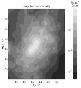
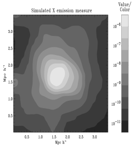
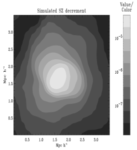
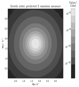
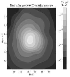
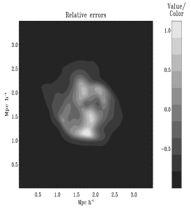
Figure 4: The upper panel shows the results of simulation, from left to right, all using a logarithmic scaling, the projected mass density ($\mathrm{M_{\sun}\ Mpc^{-2}}$), the X-ray emission measure ($\mathrm{cm^{-6}Mpc}$) and the SZ $y$ parameter. This cluster is a good candidate for our approach since it has a circular core with surrounding perturbations so would be inadequate for a ellipsoidal fit. The lower panel shows, from left to right a zeroth order predicted X emission measure, the first order prediction (the zeroth order term plus the first order correction), both using a logarithmic scaling as well as well as the the relative error map, i.e. (predicted - simulated)/simulated X emission measure using a linear scaling. The 10 error contours are linearly separated between -1.0 and 1. Each box is $3.5\ h^{-1}\mathrm{Mpc}$ wide. The correlation coefficient between the predicted and the simulated X-ray emission measure is $0.978\;$. The total flux differs only by $0.91\%$, thus even if the relative error map increases at high $R$ the total error remains small due to the great dynamical range involved.

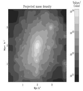
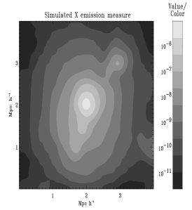
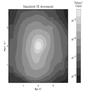
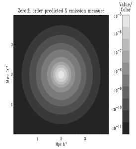
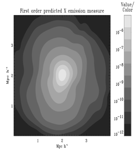
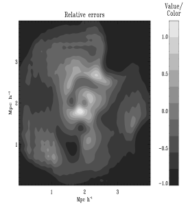
Figure 5: As the previous figure for a different cluster. The structure of the X-ray emission measure is very well reproduced for the inner part. The correlation coefficient between the predicted and simulated map is $0.986\;$. As visible on the relative error map, whose 10 levels are linearly separated between -1.0 and 1.0, the outter part is naturally smeared by our approximation. The visible 1 o’clock clump should be treated separately. Each box is $4.0\ h^{-1}\mathrm{Mpc}$ wide. The total flux differ by $9\%$.

In order to demonstrate the ability of the method in a simplified context we used some outputs of the recently developed N-body + hydrodynamics code RAMSES simulating the evolution of a $\Lambda$-CDM universe. The RAMSES code is based on Adaptative Mesh Refinement (AMR) technics in order to increase the spatial resolution locally using a tree of recursively nested cells of smaller and smaller size. It reaches a formal resolution of $12\ \mathrm{kpch^{-1}}$ in the core of galaxy clusters (see Refregier and Teyssier 2000 and Teyssier 2001, in preparation, for details). We use here the structure of $2$ galaxy cluster extracted of the simulation to generate our needed observables, i.e. X-ray emission measure, SZ decrement and projected density (or projected gravitational potential).

The relevant observables, i.e. projected mass density, SZ decrement and for comparison purpose only the X-ray emission measure, of the 2 clusters are depicted using a logarithmic scaling in figure 4 and 5 (upper panels). This clusters have been extracted of the simulation at $z=0.0$ and thus tends to be more relaxed. They are ordinary clusters of virial mass (defined by $\delta_{334}$ in our particular cosmology) $4.50\ 10^{14}\ h^{-1}\ \mathrm{M_{\sun}}$ and $4.15\ 10^{14}\ h^{-1}\ \mathrm{M_{\sun}}$. Both exhibit rather regular shape, i.e. they have not undergo recently a major merge. The depicted boxes are respectively $3.5\ h^{-1}\mathrm{Mpc}$ and $4.0\ h^{-1}\mathrm{Mpc}$ wide. We smooth the outputs using a gaussian of width $120\ h^{-1}\mathrm{kpc}$ thus degrading the resolution. We did not introduce any instrumental noise. This clusters are to a good approximation isothermal thus for the sake of simplicity we will assume that $T_{g}$ is constant making the discussion on $T_{g,0}$ and $T_{g,1}$ useless at this point. We apply the method previously described using perturbed spherical symmetry. We deduce by averaging over concentric annuli a zeroth order circular description of the gas density and then add to it some first order corrections. Note that since we assume isothermality SZ data give us straightforwardly a projected gas density modulo a temperature $T_{g,0}$ coefficient, thus we use the formulation of equation (48), exact in this context. This constant temperature is fixed using the hydrostatic equilibrium and the WL data.

In figure 4 and 5 (lower panels) we show the predicted X-ray emission measure to zeroth and first order as well as a map of relative errors. Note that to first order the shape of the emission measure is very well reproduced. The cross-correlation coefficients between the predicted and simulated X-ray emission measure are $0.978$ and $0.986$. Of course this is partly due to the assumed good quality of the assumed SZ data but nonetheless, it demonstrates the validity of our perturbative approach as well as of our approximation. The approximation performed in equation (61), i.e. the multiplication by the function $\rho_{g,0}(R)$ will naturally tends to cut out the perturbations at high $R$. This is the reason why the further perturbation are slightly less well reproduced and the relative errors tend to increase with $R$. Nevertheless, since the emission falls rapidly with $R$ as visible on the lower figures (note the logarithmic scaling) the total flux is well conserved, respectively to $0.9\ \%$ and $9\ \%$. This last number might illustrate that the large extent of the perturbations in the second case may limit our method. An ellipsoidal fit could have help decrease this value. Note that moreover the clump visible mainly in X-ray emission measure of figure 5 is not reproduce. This is natural because it does not appear through the SZ effect since the pression remains uniform throughout clumps. If resolved by WL, this substructure should anyway be treated separately, e.g. by considering the addition of a second very small structure. Note that the first cluster showed exhibits a spherical core elongated in the outter region thus it is not actually as ellipsoidal as it looks which may explain why our perturbed spherical symmetry works well.

5 Discussion

5.1 Hypothesis …and non hypothesis

Our approach makes several assumptions. Some general and robust hypothesis have been introduced and discussed in section 2.1. Note that we do not need to assume isothermality. Our key hypothesis consists in assuming the validity of a perturbative approach and in the choice of the nature of this perturbations, i.e. with a radial/angular part separation. Theoretical predictions, observations and simulations show that relaxed clusters are regular and globally spheroidal objects, which is what initially motivated our approach. Then in our demonstration on simulations, this turns out to be reasonable. Such an approach can not deal properly with sharp features as e.g. shocks waves due to infalling filaments. Then assuming the validity of the angular and radial separation, leads to the equality of this angular parts for all relevant physical quantities ($P_{g}$, $T_{g}$, $\phi_{DM}$…), using to first order in $\varepsilon$ the hydrostatic equilibrium and the equation of state. If this is not satisfied in practice then we could either question the validity of this separation or the physics of the cluster. Our experience with simulation shows that for reasonably relaxed clusters, i.e. not going through a major merge, the angular part of the perturbation is constant amongst observables. Thus it looks like the separation (and thus the equality of the angular perturbation) is a good hypothesis in general and its failure is a sign of non-relaxation, i.e. non-validity of our general physical hypothesis.

Then an important hypothesis lies in the validity of the approximation used. Note first that even if its form is general, its validity depends on the quantity which is assumed to be constant along the integral. In the case of the gas density obtained from the SZ map, it is an exact statement as soon as we assume the isothermality and since clusters in general are not too far from isothermality, this hypothesis is reasonable.

Now, some worth to remember “non hypothesis” are the isothermality and the sphericity (or ellipsoidality). This might be of importance. Indeed, in evaluating the Hubble constant from joint SZ and X-ray measurement it has been evaluated in Inagaki et al. (1995); Roettiger et al. (1997); Puy et al. (2000) that, both the asphericity and the non-isothermality of the relevant cluster can yield some important bias (up to $20\%$). Even if this measure is not our concern here, it is interesting to note that this hypothesis are not required here.

5.2 The equivalent spheroidal symmetry case

So far, we have work and discussed the perturbed spherical symmetry case. If we turn to spheroidal symmetry the problem is very similar as long as we assume the knowledge of the inclination angle $i$ between the polar axis of the system and the line of sight. This is what we recall in appendix B which is directly inspired from Fabricant et al. (1984): once the projection is nicely parametrised we get for the projected quantity , e.g. for the pressure :

$$y(\eta) = 2{B_{e}\over R}\int_{\eta}^{\infty}{P_{g,0}(t)\ tdt\over(t^{2}-\eta^{2})^{1\over 2}}$$ (62)

$$P_{g,0}(t) = -{1\over 2\pi}{R\over B_{e}}\int_{t}^{\infty}P_{g,0}^{\prime}(\eta)\,{d\eta\over\left(\eta^{2}-t^{2}\right)^{1/2}}\ .$$ (63)

following the notations of appendix B. Since we are dealing with the same Abel integral we can proceed in two steps as we did before.

Even if the inclination angle is a priori not accessible directly through single observations it has been demonstrated that it is possible to evaluate it using the deprojection of an axially symmetric distribution of either X-ray/SZ maps or SZ/surface density maps Zaroubi et al. (1998, 2000). Our approach in this work try to avoid to explicit the full 3-D structure rather than building it, and this is done in a simple self-consistent way therefore we will not get into the details of this procedure that will be discussed in a coming work (Doré et al. 2001, in preparation). Note also that axially symmetric configuration elongated along the line of sight may appear as spherical. This is a difficult bias to alleviate without any prior for the profile. In our case, our method will be biased in the sense that the deprojected profile will be wrong. Nevertheless, we might hope to reproduce properly the global quantities, like abundance of DM or gas and so to alleviate some well known systematics (see previous section), e.g. in measuring the baryon fraction.

6 Conclusion and outlook

It this paper we have presented and demonstrated the efficiency of an original method allowing to perform in a self-consistent manner the joint analysis of SZ and WL data. Using it on noise free simulation we demonstrated how well it can be used to make some x-ray surface brightness prediction, or equivalently emission measure. Our choice in this approach has been to hide somehow the deprojection by using some appropriate approximations. Thus we do not resolved fully the 3-D structure of clusters, but note that the work presented here is definitely a first step towards a full deprojection (Doré et al. 2001, in preparation). Some further refinements of the methods are under progress as well.

When applying the method to true data, the instrumental noise issue is an important matter of concern. Indeed, whereas the strong advantage of a parametric approach, e.g. using a $\beta$-model, is that it allows to adjust the relevant parameters, e.g. $r_{c}$ and $\beta$, on the projected quantities (the image) itself, which is rather robust to noise, it might be delicate to determine the profiles and its derivate by a direct deprojection. Nevertheless, our perturbative approach, as it first relies on a zeroth order quantity found by averaging over some annulus, a noise killing step (at least far from the center), and then work on some mere projected perturbation should be quite robust as well. Consequently we hope to apply it very soon on true data. Furthermore, in this context it should allow a better treatment of systematics (asphericity, non isothermality,…) plaguing any measure of the baryon fraction $f_{b}$ or the Hubble constant $\mathrm{H}_{0}$ using X-ray and SZ effect Inagaki et al. (1995). These points will be discussed somewhere else (Doré et al. 2001, in preparation ).

Annexe : Deprojection in spheroidal symmetry

In this appendix we recall some useful results concerning spheroid projection derived by Fabricant, Gorenstein and Rybicki Fabricant et al. (1984). In the context of spheroidal systems, cartesian coordinates system are the most convenient for projection. Thus, if the observer’s coordinate system $(x,y,z)$ is chosen such that the line of sight is along the $z$ axis and such that the polar axis of the spheroidal system $z^{\prime}$ lies in the $x-z$ plane at an inclination angle $i$ to the z-axis, then, in the cartesian coordinate system $(x^{\prime},y^{\prime},z^{\prime})$ the general physical quantities relevant to our problem depends only on the parameter $t$ defined by

$$t^{2} = {x^{\prime 2}+y^{\prime 2}\over B_{e}^{2}}+{z^{\prime 2}\over A_{e}^{2}}$$ (64)

$$= {(x\cos i+yz\sin i)^{2}+y^{2}\over B_{e}^{2}}+{(z\cos i-x\sin i)^{2}\over A_{e}^{2}}\>.$$ (65)

If we project a physical quantity $G(t)$ on the observer sky plane $x-y$ then,

$$I(x,y) = I(\eta)$$ (66)

$$= \int_{-\infty}^{+\infty}\ G(t)dl$$ (67)

$$= 2{B_{e}\over R}\int_{\eta}^{\infty}{G(t)\ tdt\over(t^{2}-\eta^{2})^{1\over 2}}$$ (68)

where

$$\eta^{2} \equiv {x^{2}\over(RA_{e})^{2}}+{y^{2}\over(B_{e})^{2}}$$ (69)

$$\mbox{ and }\displaystyle R \equiv \sqrt{{B_{e}^{2}\over A_{e}^{2}}\cos^{2}i+sin^{2}i}\>.$$ (70)

Of course this result shows that if we were to observe a spheroidal system we would map ellipses with an axial ratio equal to $\displaystyle{B\over A}={1\over R}{B_{e}\over A_{e}}$. But the main result of this appendix is that we obtain at the end an Abel integral similar to the one obtained in the case of spherical system, where the radius as been replaced by the parameter $t$. This simple fact justifies the very analogous treatment developed in this paper for spherical and spheroidal systems.

References

- Bartelmann and Schneider (2001) M. Bartelmann and P. Schneider, Phys. Rep., 340, 291, 2001
- Binney and Tremaine (1987) J. Binney and S. Tremaine, Princeton University Press, 1987
- Birkinshaw (1999) M. Birkinshaw, Phys. Rep., 310, 97, 1999
- Cavaliere & Fusco-Femaino (1976) A. Cavaliere and R. Fusco-Femaino, A&A, 49, 137, 1976
- Castander et al. (2000) F.J. Castander et al. , In F. Durret, D. Gerbal, editors, Constructing the Universe with clusters of galaxies, 2000
- Chièze et al. (1998) J. Chièze, J. Alimi and R. Teyssier, ApJ, 495, 630, 1998
- Désert et al. (1998) F.-X. Désert et al. , New Astronomy, 3, 655-669, 1998
- Doré et al. (2000) O. Doré et al. , In F. Durret, D. Gerbal, editors, Constructing the Universe with clusters of galaxies, 2000
- Fabian et al. (1981) A.C. Fabian et al. , ApJ, 248, 47, 1981
- Fabricant et al. (1984) D. Fabricant, G. Rybicki and P. Gorenstein, ApJ, 286, 186, 1984
- Holder et Carlstrom (1999) G. Holder and J. Carlstrom, In de Oliveira-Costa A., Tegmark M., editors, ASP Conf. Ser. 181: Microwave Foregrounds, 1999
- Holder et al. (2000) G. Holder et al. , In F. Durret, D. Gerbal, editors, Constructing the Universe with clusters of galaxies, 2000
- Grego et al. (1999) L. Grego et al. , ApJ, 539, 39, 2000
- Inagaki et al. (1995) Y. Inagaki, T. Suginohara, Y. Suto, PASJ, 47, 411, 1995
- Mellier (2000) Y. Mellier, ARA&A, 37, 127, 2000
- Puy et al. (2000) D. Puy et al. , astro-ph/0009114
- Rephaeli (1995) Y. Rephaeli, ARA&A, 33, 541, 1995
- Reblinsky and Bartelmann (1999) K. Reblinsky and M. Bartelmann, astro-ph/9909155
- Reblinsky (2000) K. Reblinsky, PhD thesis at Ludwig Maximilians Universität München, 2000
- Reese et al. (2000) E.D. Reese et al. , ApJ, 533, 38, 2000
- Réfregier and Teyssier (2000) A. Refregier and R. Teyssier, astro-ph/0012086, submitted to Phys. Rev. D
- Roettiger et al. (1997) K. Roettiger, J. Stone and R. F. Mushotzky, ApJ, 482, 588, 1997
- Sarrazin (1988) C.L. Sarazin, X-ray emission from clusters of galaxies, Cambridge University Press, 1988
- Sunyaev and Zel’dovich (1972) R. Sunyaev and I. Zel’dovich, Comments Astrophys. Space Phys., 4 ,173, 1972
- Sunyaev and Zel’dovich (1980) R. Sunyaev and I. Zel’dovich, ARA&A, 18, 537,1980
- Teyssier et al. (1997) R. Teyssier, R. Chièze and J. Alimi, ApJ, 480, 36, 1997
- Yoshikawa and Suto (1999) K. Yoshikawa and Y. Suto, ApJ, 513, 549, 1999
- Zaroubi et al. (1998) S. Zaroubi et al, ApJ Let., 500, L87+, 1998
- Zaroubi et al. (2000) S. Zaroubi et al. , astro-ph/0010508
- Zel’dovich and Sunyaev (1969) I. Zel’dovich and R. Sunyaev, Astrophys. Space Science, 4, 301, 1969