A new Monte Carlo code for star cluster simulations: I. Relaxation

We have developed a new simulation code aimed at studying the stellar dynamics of a galactic central star cluster surrounding a massive black hole. In order to include all the relevant physical ingredients (2-body relaxation, stellar mass spectrum, collisions, tidal disruption, …), we chose to revive a numerical scheme pioneered by Hénon in the 70’s (Hénon 1971b, a, 1973). It is basically a Monte Carlo resolution of the Fokker-Planck equation. It can cope with any stellar mass spectrum or velocity distribution. Being a particle-based method, it also allows one to take stellar collisions into account in a very realistic way. This first paper covers the basic version of our code which treats the relaxation-driven evolution of a stellar cluster without a central BH. A technical description of the code is presented, as well as the results of test computations. Thanks to the use of a binary tree to store potential and rank information and of variable time steps, cluster models with up to $2\times 10^{6}$ particles can be simulated on a standard personal computer and the CPU time required scales as $N_{\mathrm{p}}\ln(N_{\mathrm{p}})$ with the particle number $N_{\mathrm{p}}$. Furthermore, the number of simulated stars needs not be equal to $N_{\mathrm{p}}$ but can be arbitrarily larger. A companion paper will treat further physical elements, mostly relevant to galactic nuclei.

1 Introduction

The study of the dynamics of galactic nuclei is likely to become a field to which more and more interest will be dedicated in the near future. Numerous observational studies, using high resolution photometric and spectroscopic data, point to the presence of “massive dark objects” in the centre of most bright galaxies (see reviews by Kormendy & Richstone 1995; Rees 1997; Ford et al. 1998; Magorrian et al. 1998; Ho 1999; van der Marel 1999; de Zeeuw 2001), including our own Milky Way (Eckart & Genzel 1996, 1997; Genzel et al. 1997; Ghez et al. 1998, 1999b, 1999a; Genzel et al. 2000). As the precision of the measurements and the rigor of their statistical analysis both increase, the conclusion that these central mass concentrations are in fact black holes (BHs) with masses ranging from $10^{6}\,M_{\sun}$ to a few $10^{9}\,M_{\sun}$ becomes difficult to evade, at least in the most conspicuous cases (Maoz 1998). Hence, the time is ripe for examining in more detail the mutual influence between the central BH and the stellar nucleus in which it is engulfed.

A few particular questions we wish to answer are the following:

• What is the stellar density and velocity profile near the centre?

• What are the stellar collision and tidal disruption rates? Were they numerous enough in past epochs to contribute significantly to the growth of the central BH? Do they occur frequently enough at present to be detected in large surveys and thus reveal the presence of the BH?

• What dynamical role do these processes play? Are they just by-products of the cluster’s evolution or are there any feed-back mechanisms?

• What is the long-term evolution of such a stellar system? Will it experience core collapse, re-expansion, or even gravothermal oscillations like globular clusters?

To summarize, our central goal is to simulate the evolution of a galactic nucleus over a few $10^{9}$ years while taking into account a variety of physical processes that are thought to contribute significantly to this evolution or are deemed to be of interest for themselves. Here is a list of the ingredients we want to incorporate into our simulations:

• Relaxation induced by 2-body gravitational encounters. The accumulation of these weak encounters leads to a redistribution of stellar orbital energy and angular momentum. The role of relaxation has been extensively studied in the realm of globular clusters where it leads to the slow built-up of a diffuse halo and an increase in the central density until the so-called “gravo-thermal” catastrophe sets in (see Sect. 7.2). Of particular relevance to galactic nuclei are early studies that demonstrated that, when a central star-destroying BH is present, relaxation will lead to the formation of a quasi-stationary cusp in the stellar density (Peebles 1972; Shapiro & Lightman 1976; Bahcall & Wolf 1976; Dokuchaev & Ozernoi 1977a, b; Lightman & Shapiro 1977; Shapiro & Marchant 1978; Cohn & Kulsrud 1978).

• Tidal disruptions of stars by the BH (Rees 1988, 1990). Not only can this be a significant source of fuel for the central BH, but it can also play a role in the cluster’s evolution, as specific orbits are systematically depleted. The destruction of deeply bound stars may lead to heating the stellar cluster (Marchant & Shapiro 1980).

• Stellar collisions. As the stellar density increases in the central regions, collisions become more and more frequent. By comparing the relaxation time and the collision time (Binney & Tremaine 1987, for instance), one sees that collisions can catch up with relaxation when $\sigma_{v}>\left(\ln\Lambda\right)^{1/4}V_{\ast}\approx 1000\,\mathrm{km}\,\mathrm{s}^{-1}$, where $\sigma_{v}$ is the velocity dispersion in the stellar cluster, $\ln\Lambda$ the Coulomb logarithm and $V_{\ast}$ the escape velocity from the surface of a typical main sequence (MS) star. But even in colder clusters, collisions may be of interest as a channel to create peculiar stars (blue stragglers, stripped giants,…).

• Stellar evolution. As stars change their masses and radii, the way they are affected by relaxation, tidal disruptions and collisions is strongly modified. Of particular importance is the huge increase in cross section during the giant phase and its nearly vanishing when the star finally evolves to a compact remnant. As they are not prone to being disrupted, these compact stars may segregate towards the centre-most part of the nucleus where they may dominate the density (Lee 1995; Miralda-Escudé & Gould 2000, amongst others). Furthermore, the evolutionary mass loss (winds, planetary nebulae, SNe…) may strongly dominate the BH’s growth if this gas sinks to the centre (David et al. 1987b; Norman & Scoville 1988; Murphy et al. 1991).

• BH growth. Any increase of the BH’s mass may obviously lead to a higher rate of tidal disruptions. It also imposes higher stellar velocities and, thus, increases the relative importance of collisions in comparison with relaxation. A further contributing effect is the central density built-up due to the adiabatic adaptation of stellar orbits to the deepening potential (Young 1980; Lee & Goodman 1989; Cipollina & Bertin 1994; Quinlan et al. 1995; Sigurdsson et al. 1995; Leeuwin & Athanassoula 2000).

Although we restrict our discussion to these physical ingredients in the first phase of our work, there are many others of potential interest; some of them are mentioned in Sect. 8.2.

Thus, the evolution of galactic nuclei is a complex problem. As it is mostly of stellar dynamical nature, our approach is grounded on a new computer code for cluster dynamics. Its “core” version treats the relaxational evolution of spherical clusters. This is the object of the present paper. The inclusion of further physical ingredients such as stellar collisions and tidal disruptions will be explained in a complementary article (Freitag & Benz 2001d, see also Freitag & Benz 2001b, c). In order to obtain a realistic prescription for the outcome of stellar collisions, we compiled a huge database of results from collision simulations performed with a Smoothed Particle Hydrodynamics (SPH) code (Benz 1990). This work will be described in a third paper (Freitag & Benz 2001a).

This paper is organized as follows. In the next section, we briefly review the available numerical schemes that have been applied in the past to simulate the evolution of a star cluster and explain the reasons that led us to choose one of these methods. Sections 3 to 6 contain a detailed description of the code. Test calculations are presented in section 7. Finally, in section 8, we summarize our work and discuss future improvements.

2 Choice of a simulation method

In the previous section, we briefly reviewed the main processes that should play an important role in the evolution of galactic nuclei. To treat them realistically, any stellar dynamics code has to meet the following specifications. It must:

• Allow for non-isotropic velocity distributions. This is especially important to realistically describe the way tidal disruptions deplete very elongated orbits (the loss-cone phenomenon).

• Incorporate stars with different masses. Otherwise, mass segregation would be neglected and considering the outcome of stellar collisions properly would be impossible. Furthermore, it must be possible to make the stellar properties (mass, radius) change with time to reflect stellar evolution.

• Be able to evolve the cluster over several relaxation time-scales. The amount of required computing (“CPU”) time can be kept to a reasonable level only if individual time steps are a fraction of the relaxation time scale rather than the orbital period.

Several techniques suitable for simulations of cluster evolution have been proposed in the literature. Many textbooks and papers review these methods so we can restrict ourselves to a short overview (Binney & Tremaine 1987; Spitzer 1987; Meylan & Heggie 1997; Heggie et al. 1999; Spurzem 1999; Spurzem & Kugel 2000).

As they directly integrate the particles’ equations of motion, $N$-body simulations are conceptually straightforward and do not rely on any important simplifying assumptions. Unfortunately, to correctly compute relaxation effects, forces have to be evaluated by direct summation (see, however, Jernigan & Porter 1989; McMillan & Aarseth 1993, for possible alternatives). Hence, even with specialized hardware such as GRAPE boards (Makino 1996; Taiji et al. 1996; Spurzem & Aarseth 1996), following the trajectory of several $10^{6}$ stars over tens of relaxation times remains impossible (but see Makino 2000) for a peek at the future of such systems). A solution would be to extrapolate the results of an $N$-body simulation with a limited number of particles to a higher $N$. However, this has been shown to be both tricky and risky (McMillan 1993; Heggie 1997; Aarseth & Heggie 1998; Heggie et al. 1999). The difficulty resides in the fact that various processes (relaxation, evaporation, stellar evolution…) have time scales and relative importances that depend in different ways on the number of simulated stars. Thus, in principle, simulating a cluster of $N_{\ast}$ stars with a lower number of particles, $N\ll N_{\ast}$, could only be done if all these processes are somehow scaled to the correct $N_{\ast}$. Unfortunately, such scalings are difficult to apply, precisely because the $N$-body method treats gravitation in a direct, “microscopic” way with very little room for arbitrary adjustments. Furthermore, these modifications would rely on the same kind of theory, and hence, of simplifying assumptions, as other simulation methods.

To circumvent these difficulties, a class of methods has been developed in which a stellar cluster containing a very large number of bodies is regarded as a fluid (Larson 1970b, a; Lynden-Bell & Eggleton 1980; Louis & Spurzem 1991; Giersz & Spurzem 1994, 2000, amongst many others). Such simulations have proved to be very successful in discovering new phenomena like gravo-thermal oscillations (Bettwieser & Sugimoto 1984) but rely on many strong simplifying assumptions. Most of them are shared by Fokker-Planck and Monte Carlo methods (see next paragraphs). However, this approach, which is based on velocity-moments of the collisional Boltzmann equation, further assumes, as a closure relation, some local prescription for heat conduction through the stellar cluster. This is appropriate for a standard gas, where the collision mean free path is much smaller than the system’s size (Hensler et al. 1995). Quite surprisingly, it still seems to be valid for a stellar cluster even though the radial excursion of a typical star is not “microscopic” (Bettwieser & Sugimoto 1985; Giersz & Spurzem 1994; Spurzem & Takahashi 1995). However, we discarded such an approach because, due to its continuous nature, integrating the effects of collisions in it seems difficult.

A very popular intermediate approach is the “direct” numerical resolution of the Fokker-Planck equation (FPE) (Binney & Tremaine 1987; Spitzer 1987; Saslaw 1985, for example), either by a finite difference scheme (Cohn 1979, 1980; Lee 1987; Murphy et al. 1991; Takahashi 1995; Drukier et al. 1999, and many other works) or using finite elements (Takahashi 1993, 1995). Here again, the main difficulty resides in the treatment of collisions. From a practical point of view, these methods represent the cluster as a small set of continuous distribution functions for discrete values of the stellar mass. A realistic modeling of collisional effects would then require one to multiply the number of these mass classes, at the price of an important increase in code complexity and computation time. From a theoretical point of view, collisions don’t comply with the requirement of small orbital changes that is needed to derive the FPE.

So, we have finally turned our attention to the so-called “Monte Carlo” (MC) schemes. Even though their underlying hypotheses are similar to those leading to the FPE, being particle methods, they inherit some of the $N$-body philosophy which allows us to extend their realm beyond the set of problems to which direct FPE resolutions apply. In the Monte Carlo approach, the evolution of the (spherically symmetric) cluster is computed by following a sample of test-particles that represent spherical star shells. They move according to the smooth overall cluster (+BH) gravitational potential and are given small orbital perturbations in order to simulate relaxation. These encounters are randomly generated with a probability distribution chosen in such a way that they comply with the diffusion coefficients appearing in the FPE.

The most recently invented MC code is the “Cornell” program by Shapiro and collaborators (Shapiro 1985, and references therein) with which these authors conducted seminal studies of the evolution a star cluster hosting a central BH. At the end of each time step, the distribution function (DF) is identified with the distribution of test-particles in phase-space. Then the potential is re-computed and so are diffusion coefficients that are tabulated over phase-space. This allows us to evolve the DF one step further by applying a new series of perturbations to the test-particles’ orbits. This code features ingenious improvements, such as the ability to follow the orbital motion of test-particles threatened by tidal disruption and to “clone” test-particles in the central regions in order to improve the numerical resolution. Despite its demonstrated power, we did not adopt this technique because of its already important complexity, which would increase significantly if additional physics such as stellar collisions, a stellar mass spectrum, etc, are introduced.

Spitzer and collaborators (Spitzer 1975; Spitzer & Shull 1975a, b; Spitzer & Mathieu 1980) and Hénon (1966; 1971b; 1971a; 1973) developed simpler MC schemes which show more potential for our purpose. The simulation of relaxation proceeds through 2-body gravitational encounters between neighboring shell-like particles. The deflections are tailored to lead to the same diffusion of orbits that a great number of very small interactions would cause in a real cluster. After the encounter, the shell is placed at some radius $R$ on its modified orbit. At that time, the potential is updated so it remains consistent with the positions of the shells. The main difference between the “Princeton” code by Spitzer et al. and Hénon’s algorithm is that the former uses a fraction of the orbital time as its time step while the latter uses a fraction of the relaxation time. It follows that out-of-equilibrium dynamical processes, like violent relaxation, can be computed with the Princeton code whereas Hénon’s code can only be applied to systems in virial equilibrium, which imposes an age greatly in excess of the relaxation time. Needless to say, this restriction is rewarded by an important gain in speed. In this scheme, instead of being determined by the equations of orbital motion, the radius $R$ of a given shell is randomly chosen according to a probability distribution that measures the time spent at each radius on its orbit: $\mathrm{d}P/\mathrm{d}R\propto 1/v_{\mathrm{rad}}(R)$, where $v_{\mathrm{rad}}(R)$ is its radial velocity at $R$. $R$-dependent time steps can be used to track the huge variation of the relaxation time from the cluster’s centre to its outskirts.

We chose to follow the approach developed by Hénon to write our own Monte Carlo code. It indeed appeared as an optimal compromise in terms of physical realism and computational speed. On the one hand, it allows for all the key physical ingredients listed at the beginning of this section. On the other hand, high resolution simulations are carried out in a few hours to few days on a standard personal computer. This will enable a wide exploration of the parameter space.

Since Hénon’s work, this approach has been extensively modified and successfully applied to the study of the dynamical evolution of globular clusters by Stodółkiewicz (1982; 1986) and Giersz (1998; 2000a; 2000b). Another Hénon-like MC code has recently been written by Joshi et al. (Joshi et al. 2000; Rasio 2000; Watters et al. 2000; Joshi et al. 2001). As far as we know, however, no one ever applied this simulation method to galactic nuclei.

The Monte Carlo scheme relies on the central assumption that the stellar cluster is always in dynamical equilibrium. This is the case for well relaxed systems. Sufficient observational resolution has only recently been obtained to allow an estimate of the relaxation times in the nearest galactic nuclei. Lauer et al. (1998) report relaxation times $T_{\mathrm{rel}}$ of about $7\times 10^{11}\,\mathrm{yrs}$, $3\times 10^{9}\,\mathrm{yrs}$ and $3\times 10^{6}\,\mathrm{yrs}$ at $0.1\,\mathrm{pc}$ for M31, M32 and M33 respectively. As for the Milky Way, Alexander (1999) deduces $T_{\mathrm{rel}}\simeq 3\times 10^{9}\,\mathrm{yrs}$ at $0.4\,\mathrm{pc}$ (core radius), a value that does not change significantly at smaller radii if a $\rho\propto R^{-1.8}$ cusp model is assumed with the parametrisation of Genzel et al. (1996) for the velocity dispersion. Genzel et al. (1994) get $T_{\mathrm{rel}}\simeq 4\times 10^{7}\,\mathrm{yrs}$ for the central value but the meaning of this value is unclear, as the dynamical influence of the BH was neglected in its derivation. These few values indicate that, perhaps, only a subset of all galactic nuclei are amenable to the kind of approach we are developing. However, these very dense environments with relaxation times lower than the Hubble time are precisely the ones which expectedly lead to non-vanishing rates for the disruptive events we are primarily interested in. Furthermore, note that, contrary to the case of globular clusters, stellar evolution of a population of massive stars (e.g. in a starburst) can probably not disrupt dynamical equilibrium (through mass-loss effects) as its time scale ($\geq$ a few $10^{6}$ yrs) is longer than orbital periods in a galactic nucleus ($\leq$ a few $10^{5}$ yrs).

3 General considerations

3.1 Principles underlying code design

In our work, we focus at the long term evolution of star clusters, on time scales much exceeding the dynamical (crossing) time, $T_{\mathrm{dyn}}\simeq\sqrt{R_{\mathrm{cl}}^{3}/(GM_{\mathrm{cl}})}$, where $M_{\mathrm{cl}}$ is the cluster’s total mass and $R_{\mathrm{cl}}$ a quantity indicating its size (for instance the half-mass radius). We thus make no attempt at describing evolutionary processes that occur on a $T_{\mathrm{dyn}}$ time scale, most noticeably phase mixing and violent relaxation, which are thought to rule early life phases of stellar systems (see, for instance, section 4.7 of Binney & Tremaine 1987 or section 5.5 of Meylan & Heggie 1997 and references therein). Hence, we assume that the cluster has reached a state of dynamical equilibrium. Its subsequent evolution, driven by processes with time scales $\gg T_{\mathrm{dyn}}$ (2-body relaxation, collisions, tidal disruptions and stellar evolution), passes through a sequence of such states.

This reasonable restriction allowed Hénon to devise a simulation scheme whose time step is a fraction of the relaxation time instead of the dynamical time. Naturally, this leads to an enormous gain in computation speed compared to codes that resolve orbital processes like $N$-body programs or the Princeton Monte Carlo code (Spitzer & Hart 1971; Spitzer & Thuan 1972).

Another strong simplifying assumption the scheme heavily relies on is that of spherical symmetry. This makes the cluster’s structure effectively one-dimensional which allows a simple and efficient representation for the gravitational potential (see Sect. 5.1) and the stars’ orbits and furthermore leads to a straightforward determination of neighboring particle pairs. Of course, such a geometry greatly facilitates the computation of any quantity describing the cluster’s state, such as density, velocity dispersion and so on. An obvious drawback of this assumption is that it forbids the proper treatment of any non-spherical feature as overall rotation (Arabadjis 1997; Einsel 1998; Einsel & Spurzem 1999; Spurzem & Einsel 1999; Boily 2000), an oscillating or a binary black hole (Begelman et al. 1980; Lin & Tremaine 1980; Makino 1997; Quinlan & Hernquist 1997; Gould & Rix 2000; Merrit et al. 2000) or an accretion disk interacting with the star cluster (Syer et al. 1991; Rauch 1995; Armitage et al. 1996; Vokrouhlický & Karas 1998a, b).

In Hénon’s scheme, the numerical realization of the cluster is a set of spherical thin shells, each of which is given a mass $M$, a radius $R$, a specific angular momentum $J$ and a specific kinetic energy $T$. In the remainder of the paper, we refer to these particles as “super-stars” because we regard them as spherical layers of synchronized stars that share the same stellar properties, orbital parameters and orbital phase, whose mass is spread over the shell and which experience the same processes (relaxation, collision, …) at the same time. In recent implementations of Hénon’s method by Giersz (1998) and Joshi et al. (2000), each particle represents only one star. This avoids scaling problems connected with the computation of the rate of 2- (or many) body processes but would impose too large a number of particles for galactic nuclei simulations ($10^{6}-10^{8}$ stars). In our code, each super-star consists of many stars. Hence, a cluster containing $N_{\ast}$ stars may be represented by a smaller number of super-stars, $N_{\mathrm{SS}}<N_{\ast}$. The number of stars per super-star, $N_{\ast}/N_{\mathrm{SS}}$, is the same for every super-star, in order to conserve energy and angular momentum (as well as mass when collisions are included) when simulating 2-body processes.

The super-stars’ radii being known, the potential can be computed at any time and any place so that the orbital energies of all super-stars are straightforwardly deduced from their kinetic energies and positions. Hence the set of super-stars can be regarded as a discretized representation of the one-particle distribution function (DF) $f$ which, by virtue of Jean’s theorem, only depends on the specific orbital energy $E$ and angular momentum $J$:

$$f(\@vec{x},\@vec{v})=F(E(\@vec{x},\@vec{v}),J(\@vec{x},\@vec{v}))=F(\Phi_{\mathrm{s}}(R)+\frac{1}{2}v^{2},Rv_{\mathrm{tg}})$$

where $\@vec{x}$ and $\@vec{v}$ are the position and velocity of a star, $R=\|\@vec{x}\|$, $v=\|\@vec{v}\|$ and $v_{\mathrm{tg}}$ is the tangential component of $\@vec{v}$. However, whereas a functional expression of the DF, although a complete description of the stellar system, would impose lengthy integrations (resolution of Poisson equation, as needed in direct FP methods) to yield the gravitational potential, the Monte Carlo representation of the cluster provides it directly. From this point of view, the Monte Carlo method is closer to an $N$-body philosophy than to direct FP methods.

The main difference between the MC code and a spherical 1D $N$-body simulation is that the former does not explicitly follow the continuous orbital motion of particles which preserves $E$ and $J$. However these orbital constants, as well as other properties of the super-stars, are modified by “collisional” processes to be incorporated explicitly, namely 2-body relaxation, stellar collisions and tidal disruptions. So, in the version of the code described here, the MC simulation proceeds through millions to billions of steps, each of them consisting of the selection of super-stars (Sect. 4.2.2), the modification of their properties to simulate the effects of relaxation (Sect. 4.2) and the selection of radial positions corresponding to their new orbits (Sect. 5.2).

3.2 Physical units

In the rest of this paper, unless otherwise stated, we use the “$N$-body” units as prescribed by Heggie & Mathieu (1986). In this system,

$$\begin{array}[]{lcll}G&=&1&\mbox{\ \ (Gravitational constant)},\\ M_{0}&=&1&\mbox{\ \ (Total initial cluster mass)},\\ E_{0}&=&-1/4&\mbox{\ \ (Total initial cluster energy)}.\end{array}$$

It follows that the corresponding unit of length, $\mathcal{U}_{\mathrm{l}}$ and unit of time, $\mathcal{U}_{\mathrm{t}}$, can be expressed in any system of units as

$$\mathcal{U}_{\mathrm{l}}=\frac{GM_{0}^{2}}{-4E_{0}}\mbox{\ \ and\ \ }\mathcal{U}_{\mathrm{t}}=\frac{GM_{0}^{5/2}}{\left(-4E_{0}\right)^{3/2}}.$$ (1)

If the initial cluster’s total gravitational energy is written as

$$U_{0}=-\frac{q}{2}\frac{GM_{0}^{2}}{R_{\mathrm{h}}},$$ (2)

where $q$ is a dimension-less constant and $R_{\mathrm{h}}$ is the half-mass radius, we get, for the time unit,

$$\mathcal{U}_{\mathrm{t}}=q^{-3/2}\sqrt{\frac{R_{\mathrm{h}}^{3}}{GM_{0}}}.$$ (3)

For instance, for the often used Plummer model, with stellar density $\rho(R)\propto\left(1+(R/R_{\mathrm{P}})^{2}\right)^{-5/2}$, the “$N$-body” units are:

$$\mathcal{U}_{\mathrm{l}}=\left(\frac{16}{3\pi}\right)R_{\mathrm{P}}\mbox{\ \ and\ \ }\mathcal{U}_{\mathrm{t}}=\left(\frac{16}{3\pi}\right)^{3/2}\!\!\sqrt{\frac{R_{\mathrm{P}}^{3}}{GM_{0}}}.$$

As we study systems that are stationary on orbital time scales and whose long-term evolution is driven by relaxation, it is more adequate to adopt a time unit that scales with relaxation time rather than dynamical time:

$$\tilde{\mathcal{U}}_{\mathrm{t}}=\frac{N_{\ast}}{\ln(\gamma N_{\ast})}\mathcal{U}_{\mathrm{t}}=7.25\,q^{-3/2}T_{\mathrm{rel}}^{\mathrm{h}}$$ (4)

where $T_{\mathrm{rel}}^{\mathrm{h}}$ is the standard “half-mass” relaxation time (Spitzer 1987, p. 40).

See next section for further explanations of the relaxation time and, in particular the value of $\gamma$.

4 Relaxation.

4.1 Summary of standard relaxation theory.

The theory of relaxation in stellar systems can be found in classical textbooks (Hénon 1973; Saslaw 1985; Spitzer 1987; Binney & Tremaine 1987, for instance) and will not be presented here. However, the treatment of relaxation is the backbone of Hénon’s Monte Carlo scheme. Hence a short summary of these issues is particularly worthwhile, not only to expose the inner workings of the MC method, but also to understand the limitations it suffers from (as other statistical cluster dynamics approaches) that stem from relaxation theory’s simplifying assumptions. Furthermore, its specific advantages are also to be explained in that framework.

The basic idea behind the concept of relaxation is that the gravitational potential of a stellar system containing a large number of bodies can be described as the sum of a dominating smooth contribution ($\Phi_{\mathrm{s}}$) plus a small “granular” part ($\delta\Phi$). When only the former is taken into account, the phase-space DF of the cluster obeys the collisionless Boltzmann equation. In the long run, however, the fluctuating $\delta\Phi$ makes $E$ and $J$ slowly change and the DF evolve. The basic simplifying assumption underlying relaxation theory is to treat the effects of $\delta\Phi$ as the sum of multiple uncorrelated 2-body hyperbolic gravitational encounters with small deviation angles. Under these assumptions, if a test star “1” travels through a homogeneous field of stars “2” which all share the same properties (masses and velocities) during $\delta t$, its trajectory will deviate from the initial direction by an angle $\theta$ with the following statistical properties:

$$\left\langle\theta\right\rangle_{\delta t} = 0,$$

$$\left\langle\theta^{2}\right\rangle_{\delta t} \simeq 8\pi n\ln\left(\frac{b_{\mathrm{max}}}{b_{0}}\right)\frac{G^{2}\left(M_{1}+M_{2}\right)^{2}}{v_{\mathrm{rel}}^{3}}\>\delta t.$$ (5)

In this equation, $n$ is the number density of stars, $M_{1}$ the mass of the test star, $M_{2}$ the mass of each field-star, $v_{\mathrm{rel}}$ the relative velocity between the test star and the field stars, $b_{0}$ is the impact parameter leading to a deviation angle of $\pi/2$ and $b_{\mathrm{max}}$ is a cut-off parameter needed to avoid a logarithmic divergence. This ill-defined value represents the largest possible impact parameter and is thus expected to be of the order of the size of the stellar system, $R_{\mathrm{cl}}$. If $\sigma_{v}$ is the velocity dispersion in the cluster and $M_{\ast}$ the average stellar mass, the argument of the so-called “Coulomb logarithm” can be approximated by

$$\frac{b_{\mathrm{max}}}{b_{0}}\simeq\frac{v_{\mathrm{rel}}^{2}R_{\mathrm{cl}}}{G\left(M_{1}+M_{2}\right)}\simeq\frac{\sigma_{v}^{2}R_{\mathrm{cl}}}{GM_{\ast}}\simeq\gamma\frac{M_{\mathrm{cl}}}{M_{\ast}}=\gamma N_{\ast}$$ (6)

where $\gamma$ is a non-dimensional proportionality constant. This proportionality only holds for a self-gravitating, virialized cluster. The exact value of $b_{\mathrm{max}}/b_{0}$ is of little importance as it is embedded into a logarithm. Hence, in most applications, a constant $\gamma$ is used whose value is determined either from theoretical arguments (Spitzer & Hart 1971; Hénon 1975) or by $N$-body simulations (Giersz & Heggie 1994a, 1996; Drukier et al. 1999). The latter approach supports the classical “weak encounters” relaxation theory described here by showing good agreement with it for properly fitted $\gamma$ values. Furthermore it confirms Hénon (1975) who derived $\gamma\simeq 0.10-0.17$ for single mass clusters and demonstrated the need for a much smaller value when an extended stellar mass spectrum is treated. Here, we use $\gamma=0.14$ and $\gamma=0.01$ respectively.

As Eq. 5 is of central importance for the simulation of relaxation in the Monte Carlo code, we comment on the main assumptions on which its derivation relies. First, as already stated, deflections are assumed to be of very small amplitude and uncorrelated with each other. The contribution of encounters with impact parameters between $b_{1}$ and $b_{2}$ is of order $\ln\left(b_{2}/b_{1}\right)$ so equal logarithmic intervals of $b$ contribute equally to $\left\langle\theta^{2}\right\rangle$ and most of the relaxation is indeed created by “distant encounters”: $b\gg b_{0}\Rightarrow\theta\ll\pi/2$.

Moreover, the derivation applies in principle only to homogeneous systems with a finite size. However, a real cluster is grossly inhomogeneous, with large density gradients. Applying Eq. 5 for realistic clusters forces us into assuming the “local approximation”, i.e. stating that typically $b\ll R_{\mathrm{cl}}$. Then, not only can we neglect the effect of $\Phi_{\mathrm{s}}$ during an encounter and treat the trajectories as Keplerian hyperbolae, but, as an added benefit, we can use the local properties of the cluster (density and velocity distribution) as representative of field stars met by the test-particle. Admittedly, this is a bold assumption only partially justified by the “$\ln(b_{2}/b_{1})$” argument. The validity of these approximations has been assessed by comparing results of codes based on relaxation theory with $N$-body simulations which do not rely on such assumptions (Giersz & Heggie 1994a; Spurzem & Aarseth 1996; Giersz 1998; Portegies Zwart et al. 1998; Takahashi & Portegies Zwart 1998; Spurzem 1999).

Recasting Eqs. 5, 6 into

$$\left\langle\theta^{2}\right\rangle_{\delta t}\simeq\left(\frac{\pi}{2}\right)^{2}\frac{\delta t}{\widehat{T}_{\mathrm{rel}}^{(1,2)}},$$ (7)

we define

$$\widehat{T}_{\mathrm{rel}}^{(1,2)}=\frac{\pi}{32}\frac{v_{\mathrm{rel}}^{3}}{\ln\left(\gamma N_{\ast}\right)G^{2}n\left(M_{1}+M_{2}\right)^{2}}.$$ (8)

We call this quantity the “encounter relaxation time” to insist on its depending on the properties of one particular class of encounters, namely those between stars of mass $M_{1}$ and stars of mass $M_{2}$ of (local) density $n$ with relative velocity $v_{\mathrm{rel}}$. It can be loosely interpreted as the time needed for encounters with stars “2” to gradually deflect the direction of motion of star “1” by a RMS angle $\pi/2$.

4.2 Monte Carlo simulation of relaxation.

4.2.1 Elementary numerical encounter.

Contrary to Fokker-Planck codes, Hénon’s method was devised to avoid the computational burden and the necessary simplifications connected with the numerical evaluation of diffusion coefficients (DCs). It does so through a direct use of Eq. 5 whose repeated application to a particular super-star “1” is equivalent to a Monte Carlo integration of the DCs, provided the properties of field particles “2” are correctly sampled. Under the usual assumption that encounters are local, this latter constraint is obeyed if we take these properties to be those of the closest neighboring super-star. Furthermore, this allows us to actually modify the velocities of both super-stars at a time, each one acting as a representative from the “field” for the other. Hence, in the Hénon code (as well as in ours), super-stars are evolved in symmetrical pairs. This does not only speed up the simulations by a factor $\simeq 2$, but also ensures proper local conservation of energy, a feature which turned out to be a prerequisite for correct cluster evolution. Unfortunately this pairwise approach also impose heavy constraints on the code’s structure and (perhaps) abilities as we shall show later on.

So the elementary ingredients in the heart of Hénon’s scheme are simulated 2-body gravitational deflections between neighboring super-stars. However, instead of being direct one-to-one counterparts to real individual encounters – which would lead to much too slow a code with a (huge) number of computational steps scaling as $N_{\mathrm{part}}^{2}$ – these are actually “super-encounters”, devised to statistically reproduce the cumulative effects of the numerous physical deflections taking place in the real system over a time span $\delta t$. Thus, such a numerical encounter has a double nature. First, it is computed as a (virtual) 2-body gravitational interaction with deflection angle $\theta_{\mathrm{SE}}$ in the pair CM frame. But being in charge of representing all the (small-angle) deflections that test-star “1” experiences during $\delta t$ when meeting field-stars “2”, it also has to obey Eqs. 7, 8. Consequently, $\theta_{\mathrm{SE}}$ has to equate the root mean squared cumulative deflection

$$\theta_{\mathrm{SE}}=\frac{\pi}{2}\sqrt{\frac{\delta t}{\widehat{T}_{\mathrm{rel}}^{(1,2)}}}.$$ (9)

This double nature of the encounter is reflected in the whole MC scheme that can be regarded either, quite abstractly, as a stochastic algorithm to solve the Fokker-Planck equation or, more simply, as some kind of randomized N-body scheme. The second viewpoint, though it might be misleading on certain occasions, is the one we usually adopt as it allows more intuitive reasoning.

We now describe the computation of a particular numerical encounter. It decomposes into the following steps:

1. A pair of adjacent super-stars and a time step $\delta t$ are chosen by a procedure to be explained in Sect. 4.2.2.

2. The local density $n$ entering the determination of $\widehat{T}_{\mathrm{rel}}^{(1,2)}$ in Eq. 9 is estimated.

3. The super-stars’ velocities, $\@vec{v}_{1}$ and $\@vec{v}_{2}$ are randomly oriented while respecting the angular momenta $J_{i}=\|\@vec{J_{i}}\|$ and specific kinetic energy $T_{i}=\frac{1}{2}\@vec{v_{i}}^{2}$ of both super-stars. This sets the CM- and relative velocities $\@vec{v}_{\mathrm{CM}}$ and $\@vec{v}_{\mathrm{rel}}$. The former defines the encounter CM frame while the latter allows $\theta_{\mathrm{SE}}$ to be determined through Eqs. 8 and 9.

4. In the CM frame, the orientation of the orbital plane is randomly chosen around the direction of $\@vec{v}_{\mathrm{rel}}$. $\theta_{\mathrm{SE}}$ being known, computing the post-encounter velocities in the CM frame is trivial.

5. These velocities are transformed back to the cluster frame where they define new $J_{i}$s and $T_{i}$s for both super-stars.

To compute the local density of star $n(R)$ required in step 1, we build and maintain a radial “Lagrangian” mesh each of whose cells typically contains a few tens of super-stars. The cells’ radial limits are known, as well as the number of super-star they contain. Hence, an estimate of the local number density is easily computed by dividing the total number of stars in the cell where the encounter takes place by its volume. Frequent updating (after each super-star orbital movement) and occasional rebuilding of the mesh introduces only a very slight computational overhead, most CPU time being spent in binary tree traversals during potential and rank computations (see Sect. 5.1).

The computations in steps 2-4 are described in appendix C. The only physical content of all this procedure resides in the determination of $\theta_{\mathrm{SE}}$. Everything else is a matter of elementary frame transformations and correct random sampling of free parameters in the Monte Carlo spirit.

4.2.2 Choice of the relaxation pair. Determination of the time step.

With no other physical process than relaxation included, each individual step in our algorithm comprises three operations:

1. Selection of a pair of neighboring super-stars to be evolved.

2. Modification of their orbital properties ($E_{i}$ and $J_{i}$) through a super-encounter, as explained above.

3. For each super-star, selection of a new position on the ($E_{i}^{\prime}$,$J_{i}^{\prime}$)-orbit, i.e. determination of a new radius $R_{i}$ for the spherical shell. This comprises an adequate update of the cluster’s potential.

At that point, the code cycles back to 1, i.e., another pair is chosen and another step begins. This crucial selection process is presented in this section.

The choice procedure is mainly constrained by the necessity of allowing super-stars to have individual time-steps $\delta t_{i}$ that reflect the enormous variations of the relaxation time between the central and outer parts of the stellar cluster. When collisions are included, the dynamical range of evolution times can be even larger. Unless this specification is met, the code’s efficiency would be very low as the overall $\delta t$ would have to reflect the very short central evolution time. One could also be concerned by the orbital time exceeding $\delta t$ for a large fraction of super-stars, a situation inconsistent with the “orbital average” approach implicitly assumed in the Monte Carlo scheme. However, this problem is actually nonexistent in a purely relaxational system whose evolution – under the assumptions made in the standard relaxation theory – is independent of $T_{\mathrm{relax}}/T_{\mathrm{dyn}}$, provided $N_{\ast}$ is large enough ($\gg 100$).

The other important constraint is the need to evolve both super-stars in an interacting pair. If the same time step is not used for both super-stars, energy is not conserved and a very poor cluster simulation ensues. But adjacent super-stars only form a pair during a unique interaction and then break apart as each one is attributed a new radius. So, momentary neighboring super-stars have to be given similar $\delta t_{i}$. This strongly suggests use of local time steps, i.e. $\delta t$ should be a function of $R$ alone.

Naturally, the time steps have to be sufficiently smaller than the time scale for the physical processes driving the cluster evolution, namely the relaxation in the present case. Hence, we impose:

$$\delta t(R)\leq\delta t_{\mathrm{opt}}(R)=f_{\delta t}\tilde{T}_{\mathrm{rel}}(R)$$ (10)

where $\tilde{T}_{\mathrm{rel}}$ is some kind of locally averaged relaxation time defined as (see Eq. 8):

$$\tilde{T}_{\mathrm{rel}}\propto\frac{\langle v^{2}\rangle^{\frac{3}{2}}}{\ln\left(\gamma N_{\ast}\right)G^{2}n\langle M_{\ast}\rangle^{2}}$$ (11)

and $f_{\delta t}=0.005-0.05$ typically.

In Eq. 11, $n$ (star number density), $\langle v^{2}\rangle$ (average squared velocity) and $\langle M_{\ast}\rangle$ (average stellar mass) are $R$-dependent properties of the cluster. As the only role of $\tilde{T}_{\mathrm{rel}}$ is to provide short enough $\delta t_{i}$s, an approximate evaluation of these quantities (using a coarse mesh or a sliding average) is sufficient. On the other hand, too short $\delta t_{i}$s would fruitlessly slow down the code and should be avoided by considering $\delta t_{\mathrm{opt}}$ in Eq. 10 not only as an upper limit for the time step but also as an optimal value to be approached as closely as possible.

As the members of a pair arrived at their present position at different times but have to leave it at the same time, once the super-encounter is performed, imposing the same $\delta t$ to both super-stars is impossible. So, building on the statistical nature of the scheme, instead of trying to maintain a super-star at radius $R$ during exactly $\delta t(R)$, we only require the mean waiting time for super-stars at $R$ to be $\delta t(R)$. As explained by Hénon (1973), this constraint is fulfilled if the probability for a pair lying at $R$ to be selected and evolved (and thus, taken away from $R$) during a time span $dt$ is $P_{\mathrm{selec}}(R)=dt/\delta t(R)$. This is realised in the following way:

• As it would be difficult to define and use a selection probability $P_{\mathrm{selec}}$ which is a function of the continuous variable $R$, we define it to depend on the rank $i$ of the pair (rank 1 designates the two super-stars that are closest to the centre, rank 2 the second and third super-stars, in ascending order of $R$ and so on). For a given cluster’s state, local relaxation times $\tilde{T}_{\mathrm{rel}}$ are computed at the radial position of every pair. Rank-depending time steps are defined that obey inequality 10,

  $$\delta t(i)\leq f_{\delta t}\tilde{T}_{\mathrm{rel}}(R(i)).$$ (12)

• Normalized selection probabilities are computed,

  $$P_{\mathrm{selec}}(i)=\frac{\overline{\delta t}}{\delta t(i)}\mbox{\ \ with\ \ }\overline{\delta t}=\left(\sum_{j=1}^{N_{\mathrm{SS}}-1}\frac{1}{\delta t(j)}\right)^{-1}$$ (13)

  from which we derive a cumulative probability,

  $$Q_{\mathrm{selec}}(i)=\sum_{j=1}^{i}P_{\mathrm{selec}}(j).$$ (14)

• At each evolution step another super-star pair is randomly chosen according to $P_{\mathrm{selec}}$. To do this, a random number $X_{\mathrm{rand}}$ is first generated with uniform probability between 0 and 1. The pair rank is then determined by inversion of $Q_{\mathrm{selec}}$:

  $$i=Q_{\mathrm{selec}}^{-1}(X_{\mathrm{rand}}).$$ (15)

  The binary tree (See Sect. 5.1) is traversed twice to find the id-numbers of the member super-stars whose (momentary) ranks are $i$ and $i+1$.

• The pair is evolved through a super-encounter, as explained in Sect. 4.2.1, for a time step $\delta t(i)$.

• After a large number of elementary steps, typically $0.5\,N_{\mathrm{SS}}$, the $\delta t(i)$ and $P_{\mathrm{selec}}(i)$ are re-computed from scratch to reflect the slight modification of the overall cluster structure.

Figure 1: Selection probability in a Plummer cluster consisting of 4000 super-stars. Solid curves correspond to $P_{\mathrm{selec}}\propto 1/T_{\mathrm{rel}}$, dashed ones to Hénon’s recipe and dot-dashed ones to our piecewise approximation.

As evaporation, collisions and tidal disruptions remove stars from the cluster, the number of super-stars $N_{\mathrm{SS}}$ generally decreases between two successive computations of the selection probabilities. To avoid this problem, $\delta t$, $P_{\mathrm{selec}}$ and $Q_{\mathrm{selec}}$ are actually defined as functions of $x_{\mathrm{rank}}=i/N_{\mathrm{SS}}\in]0,1]$.

For the sake of efficiency, we should manage to get for $Q_{\mathrm{selec}}^{-1}$ a function that is quickly evaluated. We explored two solutions. We first mimicked Hénon’s recipe, using the functional forms:

$$P_{\mathrm{selec}}(i) = \frac{(1+C)CN_{\mathrm{SS}}}{(i+CN_{\mathrm{SS}})(i+CN_{\mathrm{SS}}-1)}$$ (16)

$$Q_{\mathrm{selec}}(i) = \frac{(1+C)i}{i+CN_{\mathrm{SS}}}$$ (17)

$$Q_{\mathrm{selec}}^{-1}(x) = \left\lfloor 1+\frac{CN_{\mathrm{SS}}}{1+C-x}\right\rfloor$$ (18)

$$\delta t(i) = \frac{\overline{\delta t}}{P_{\mathrm{selec}}(i)}.$$ (19)

The parameter $C>0$ controls the probability contrast between the centre (short $T_{\mathrm{rel}}$ and $\delta t$) the outer regions (long $T_{\mathrm{rel}}$ and $\delta t$). The lower the value of $C$, the more centrally peaked is $P_{\mathrm{selec}}$. We determine $C$ by least-square fitting $Q_{\mathrm{selec}}(i)$ to $Q_{\mathrm{rel}}(i)\propto\sum_{j=1}^{i}T_{\mathrm{rel}}^{-1}(j)$.

However, being rather arbitrary, Hénon’s parameterization could lead to values of $\delta t$ that poorly match the shape of $T_{\mathrm{rel}}(R)$ with the effect of forcing low $\overline{\delta t}$ and hence slowing down the simulation. This concern motivated another approach. The full rank range is sliced in a few (typically 20) bins, in each of which the selection probability is set to a constant (either proportional to the maximum of $T_{\mathrm{rel}}^{-1}$ in the bin or to its mean value). Such a piecewise approximation is naturally expected to adjust better to any cluster structure, as shown in Fig. 1.

An additional constraint to be mentioned is the need to restrict the ratio of the longest time step to the shortest one, $\delta t_{\mathrm{max}}/\delta t_{\mathrm{min}}$, to ensure that the outermost shells (the cluster’s halo) evolves correctly. Otherwise these super-stars, most probably placed near their apo-centre positions, where relaxation (and, hence selection probability) is vanishing, would never be given any opportunity to visit more central regions where they can react to the adiabatic relaxation-induced modification of the central potential and experience 2-body encounters. Finally, for reasons to be presented in appendix B, it is necessary that the selection probability is a decreasing function of $R$ (i.e. of the rank). In practice, these added constraints are applied to modify unnormalised selection probabilities which are then rescaled to 1. Once the probabilities have been worked out, we ensure inequality 10 is satisfied everywhere by setting

$$\overline{\delta t}=f_{\delta t}\,\max(T_{\mathrm{rel}}(i)\cdot P_{\mathrm{selec}}(i)),$$ (20)

where the maximum is taken over all super-stars.

Figure 2: Evolution of the time dispersion of super-stars during the simulation of a core-collapsing cluster. Left panel: Time versus step number. The median time $t_{\mathrm{med}}$ is shown as a solid line. Dotted lines depict the interval $[t_{\mathrm{med}}-\Delta t_{-};t_{\mathrm{med}}+\Delta t_{+}]$ comprising $2/3$ of super-stars. Right Panel: time evolution of the relative time “dispersion” $\Delta t/t_{\mathrm{med}}$ with $\Delta t=0.5(\Delta t_{-}+\Delta t_{+})$.

As super-stars are randomly chosen to be evolved and advanced in time, strict synchronization is never realized (except at $t=0$). Each super-star $k$ has its own individual time $t^{(k)}$ and synchronization is only achieved statistically by requiring that, at every stage in the cluster’s evolution, the expectation values $E(t^{(k)})$ of all $t^{(k)}$s are the same. An equivalent statement is to impose an equal expectation value $E_{\mathrm{step}}\left(\delta t^{(k)}\right)$ for the individual time increase of any super-star during any evolution step. At the beginning of a given step, the super-stars are ranked according to their distance to the centre. Selection probability and time step depend only on the rank number $i(k)$ so that

$$E_{\mathrm{step}}\left(\delta t^{(k)}\right)=\underbrace{P_{\mathrm{selec}}(i)}_{\parbox{56.9055pt}{\centering\scriptsize\vspace{-0.3cm} Probability for selecting the super-star with rank $i$. \@add@centering}}\times\underbrace{\delta t(i)}_{\parbox{56.9055pt}{\centering\scriptsize\vspace{-0.3cm} Time step for this rank. \@add@centering}}$$ (21)

and Eq. 19 yields:

$$E_{\mathrm{step}}\left(\delta t^{(k)}\right)=P_{\mathrm{selec}}(i)\frac{\overline{\delta t}}{P_{\mathrm{selec}}(i)}=\overline{\delta t}\leavevmode\nobreak\ \leavevmode\nobreak\ \forall k$$ (22)

as desired. Figure 2 illustrates how the dispersion of super-stars’ times evolves during a typical simulation. We define the global, “cluster” time to be the median value of the super-stars’ times.

5 Orbital displacements and potential updating.

5.1 Potential representation

In Sect. 4.1, we explain how relaxation theory, as adopted in this work, relies on the assumption that the cluster’s gravitational potential $\Phi$ can be described as a dominating smooth contribution $\Phi_{\mathrm{s}}$ whose evolution time scale is much longer than the typical orbital time plus a relatively small fluctuating $\delta\Phi$. This latter contribution being further reduced to the sum of numerous 2-body encounters, we are left with the numerical representation of $\Phi_{\mathrm{s}}$.

As spherical symmetry introduces many simplifications, going beyond this central approximation deeply built into Hénon’s scheme, seems nearly impossible. Its most prominent merit is to ensure that stellar orbits, when considered on time scales much shorter that $T_{\mathrm{relax}}$, are easily dealt-with planar rosettes. Therefore, angular $\Phi$-fluctuations are removed by construction and we represent $\Phi_{\mathrm{s}}$ as the sum of the contributions of the super-stars, i.e., spherical infinitely thin shells of stars. As a consequence, radial graininess is still present but its effect turns out to be insignificant compared to “genuine” relaxation. To support this claim, we switched off simulated physical relaxation and got a cluster showing no sign of evolution (apart from Monte Carlo noise) for a number of steps at least three times larger than needed to accomplish deep core collapse when relaxation is included.

Between two successive super-stars of rank $i$ and $i+1$, the smooth potential felt by a thin shell of mass $M$ with radius $R\in[R_{i},R_{i+1}]$ is then simply

$$\Phi_{\mathrm{s}}(R)=-\frac{A_{i}-0.5M}{R}-B_{i}$$

$$\mbox{with}\leavevmode\nobreak\ A_{i}=M_{\mathrm{BH}}+\sum_{j=1}^{i-1}M_{j}\leavevmode\nobreak\ \mbox{and}\leavevmode\nobreak\ B_{i}=\sum_{j=i}^{N_{\mathrm{SS}}}\frac{M_{j}}{R_{j}}$$

where $M_{j}$ and $R_{j}$ are the mass and radius of the super-star of rank $j$ and $M_{\mathrm{BH}}$ is the mass of the central BH. The term $0.5M/R$ is due to shell self-gravitation. To lighten notations, from this point on, $\Phi_{\mathrm{s}}$ will simply be referred to as the “potential” and the symbol $\Phi$ is re-attributed to it.

At each step in the numerical simulation, two super-stars are evolved which are given new radii and masses (if collisions or stellar evolution is simulated). An easy way of obtaining exact overall energy conservation and proper account of the adiabatic energy drift of super-stars is to update the $A_{i}$ and $B_{i}$ coefficients after every such orbital displacement. Doing so also ensures that we never put a super-star at a radius which turns out to be forbidden (either lower than peri-centre or larger than apo-centre) in the updated potential. To sum it up, this choice spares us much trouble connected with a potential that lags behind the super-star distribution. Stodołkiewicz (1982) and Giersz (1998) describe these difficulties, as well as recipes to overcome them in their programs. Similar problems are certainly present in the code of Joshi et al. (2000) as they recompute the potential only after all the super-stars have been assigned new radii. However, performing potential updates only after a large number of super-star moves has advantages of its own. In particular, in such a code, the computing time should scale linearly with the number of super-stars (for a complete cluster evolution). This also allows them to develop parallelized versions of the Monte Carlo scheme (Joshi et al. 2000).

If we implement the $A_{i}$s and $B_{i}$s as linear arrays, however, a large fraction of their $N_{\mathrm{SS}}$ elements would have to be modified after each step, so the number of numerical operations required to evolve the system to a given physical time would scale like $N_{\mathrm{SS}}^{2}$. This steep dependency could be avoided by using a binary tree data structure to store the potential (and ranking) information (Sedgewick 1988). This essential adaptation was alluded to by Hénon himself (Hénon 1973) who never published it though.

At any given time, each super-star is represented by a node in the tree. Each node is connected to (at most) two other nodes that we shall call his left and right children, which are themselves, when present, the “roots” of their father’s left and right “sub-trees”. The rules underlying the tree structure are that all the nodes in the left “child-tree” of a given node correspond to super-stars with lower radii and all the nodes in its right “child-tree” to super-stars with higher radii. If we define $\mathcal{LT}_{k}$ and $\mathcal{RT}_{k}$ to be the sets of nodes in the left and right child-trees of node $k$, then

$$R_{k} \geq R_{m}\;\;\forall m\in\mathcal{LT}_{k} R_{k} < R_{m}\;\;\forall m\in\mathcal{RT}_{k}.$$

Figure 3: Diagram of a binary tree with 12 super-stars showing node properties that encode potential ($\delta A_{k}$, $\delta B_{k}$) and rank ($\delta i_{k}$) information.

The spherical potential is represented by $\delta A_{k}$ and $\delta B_{k}$ coefficients attached to nodes. A third value, $\delta i_{k}$, allows the determination of the radial rank of any super-star. These properties, illustrated in Fig. 3, are defined by

$$\delta i_{k} = 1+\mbox{number of nodes in\leavevmode\nobreak\ }\mathcal{LT}_{k}, \delta A_{k} = M_{k}+\sum_{m\in\mathcal{LT}_{k}}M_{m}\mbox{\leavevmode\nobreak\ \leavevmode\nobreak\ and} \delta B_{k} = \frac{M_{k}}{R_{k}}+\sum_{m\in\mathcal{RT}_{k}}\frac{M_{m}}{R_{m}}.$$

Then, the super-star with rank $i$ can be found and its potential coefficients $A_{i}$ and $B_{i}$ can be computed by traversing the tree from root to the node associated with this particle. During the same traversal, the $\delta A_{k}$s, $\delta B_{k}$s and $\delta i_{k}$s of the visited nodes may be modified in order to account for the removal of this super-star. After the super-star has been given a new radius (see Sect. 5.2), it is re-introduced into the tree through another traversal. Hence, the potential and rank coefficients reflect always exactly the positions (and masses) of all the super-stars. The potential at any radius, as well as the peri- and apo-centre distances of a given super-star, can be computed by specific tree traversal routines. The number of operations involved in any of these tree traversals is proportional to the number of levels i.e., if the tree is kept reasonably well balanced, $\mathcal{O}(\log_{2}(N_{\mathrm{SS}}))$. From time to time, (typically after every super-star has been evolved 2 times on average), the binary tree is rebuilt from scratch, in order to keep it well balanced and to remove empty nodes. More details about the implementation of this binary tree can be found in appendix C.

5.2 Selection of a new orbital position

Let’s consider a star with known energy $E$ and angular momentum $J$ orbiting in a spherically symmetric potential $\Phi(R)$. Its distance to the centre $R$ oscillates between $R_{\mathrm{p}}$ (peri-centre radius) and $R_{\mathrm{a}}$ (apo-centre radius) which are the two solutions of the equation

$$v_{\mathrm{rad}}^{2}=2E-2\Phi(R)-\frac{J^{2}}{R^{2}}=0.$$ (26)

During a complete orbit the time spent in radius interval $[R,R+\mathrm{d}R]$ is $\mathrm{d}t\propto v_{\mathrm{rad}}^{-1}(R)\mathrm{d}R$ so that the probability density for finding the star at $R$ at any random time (or at a given time but without any knowledge about the orbital phase) is

$$\frac{\mathrm{d}P_{\mathrm{orb}}}{\mathrm{d}R}=\frac{2}{P_{\mathrm{orb}}}\frac{1}{v_{\mathrm{rad}}(R)}$$ (27)

where $P_{\mathrm{orb}}=2\int_{R_{\mathrm{p}}}^{R_{\mathrm{a}}}\mathrm{d}R\,v_{\mathrm{rad}}^{-1}$ is the orbital period.

Our Monte Carlo scheme avoids explicit computation of the orbital motion. It instead achieves correct statistical sampling of the orbit of any given super-star by ensuring that the expectation value for the fraction of time spent at $R$ complies with Eq. 27. Let the sought-for probability of placing the super-star at $R\in[R_{\mathrm{p}},R_{\mathrm{a}}]$ be $f_{\mathrm{plac}}(R)=\mathrm{d}P_{\mathrm{plac}}/\mathrm{d}R$. According to Eq. 19, if the super-star is placed at $R$, it will stay there for an average time $\overline{\delta t}/P_{\mathrm{selec}}(R)$. Then, combining both relations, the average ratio of times spent at two different radii $R_{1},R_{2}$ on the orbit is

$$\left\langle\frac{t_{\mathrm{stay}}(R_{1})}{t_{\mathrm{stay}}(R_{2})}\right\rangle = \frac{f_{\mathrm{plac}}(R_{1})P_{\mathrm{selec}}(R_{2})}{f_{\mathrm{plac}}(R_{2})P_{\mathrm{selec}}(R_{1})}$$ (28)

$$= \frac{v_{\mathrm{rad}}(R_{2})}{v_{\mathrm{rad}}(R_{1})}\mbox{\leavevmode\nobreak\ \leavevmode\nobreak\ as required by Eq.\leavevmode\nobreak\ \ref{eq:dPorbdR}.}$$ (29)

As a result, this imposes

$$f_{\mathrm{plac}}(R)\propto\frac{P_{\mathrm{selec}}(R)}{v_{\mathrm{rad}}(R)}.$$ (30)

In appendix B, we explain how we implement such a probability function in an efficient way.

6 Other ingredients

6.1 Evaporation and tidal truncation

Despite its long history, the theoretical understanding of the processes leading stars to escape a stellar cluster is still not complete (Binney & Tremaine 1987 Sect. 8.4.1; Meylan & Heggie 1997 Sect. 7.3; Heggie 2000). Even without considering interaction with binaries, the global picture seems a bit confusing. Nevertheless, for an isolated cluster, the basic mechanism is obvious to grasp, at a “microscopic” description level: a star can escape after it has experienced a 2-body encounter which resulted in an energy gain large enough to unbound it, i.e., to get to positive energy. Much of the confusion about the prediction of overall escape rates amounts to figuring out whether rare large angle scatterings that are neglected by the standard relaxation theory could dominate this rate. Indeed it can be argued that, in an isolated cluster, stars that are only slightly bound and could be kicked away by weak scatterings populate orbits with huge periods and spend most time near the apo-centre where encounters are vanishingly rare (Hénon 1960). According to that picture, the escape rate could not be predicted by the “standard” relaxation theory, because individual “not-so-small” angle scatterings would dominate it.

If this is true, as the MC treatment of 2-body encounters relies on the assumption of small relative changes in orbital parameters, the method cannot be expected to give reliable results for the escape rate from an isolated cluster (Hénon 1971a). Some numerical solution to that problem was introduced by Giersz (1998). However, when the cluster’s initial conditions are set to represent a galactic nucleus, the fraction of stars that evaporate during $10^{10}$ years is very small, so that a precise account of this phenomenon is not really required. It would anyway not make much sense to devise a complicated treatment of evaporation from the nucleus while we neglect the inverse process, i.e. the capture of stars from the galactic bulge. Our procedure is simply to remove any star whose energy is positive after a relaxation/collision process. As can be seen in Fig. 6, this simple prescription leads to an amount of evaporation in good agreement with the result of Giersz (1998).

However, for the sake of comparison with globular cluster simulations, we also introduced the effects of an external (galactic) tidal field. Due to the sphericity constraint, the three dimensional nature of such a perturbation cannot be respected. We resort to the usual radial truncation approach and consider that a super-star with apo-centre radius larger than the so-called tidal radius $R_{\mathrm{tid}}$ immediately leaves the cluster. The value of $R_{\mathrm{tid}}$ is about the size of the cluster’s Roche lobe, $R_{\mathrm{tid}}=cR_{\mathrm{gal}}(M_{\mathrm{cl}}/M_{\mathrm{gal}})^{1/3}$ with $R_{\mathrm{gal}}$ being the distance to the centre of the parent galaxy whose mass is $M_{\mathrm{gal}}$ and $c$ is of order unity. This criterion is clearly a quite unrealistic simplification but we do not question it in our work as it is used only for comparison purposes. As the transition from an apo-centre radius slightly below $R_{\mathrm{tid}}$ to a value slightly larger does not imply large changes in the shape of the orbit, the escape rate in this model is certainly dominated by small angle, diffusion-like relaxation and must be correctly captured by our MC approach.

6.2 Neglect of binary processes

The formation, evolution and dynamical role of binaries in star clusters are complex and fascinating subjects. An impressive number of works have been aimed at the study of binaries in globular clusters (see, for instance Hut et al. 1992, for a review). On the other hand, not much has been done concerning galactic nuclei (see Gerhard 1994).

From a dynamical point of view, only hard binaries, i.e. star couples whose orbital velocity $v_{\mathrm{orb}}$ is larger than the velocity dispersion $\sigma_{v}$ in the cluster, have to be considered. In dense systems, they act as a heat source by giving up orbital energy and contract (thus hardening further) during interactions with other stars. Of course, the fraction of primordial binaries to be labeled as “hard” is a priori much higher in globular clusters ($\sigma_{v}$ of order $10\,\mathrm{km\,s}^{-1}$) than in galactic nuclei ($\sigma_{v}\geq 100\,\mathrm{km\,s}^{-1}$). Binaries can also be formed dynamically, either by tidal energy dissipation during a close 2-body encounter (“tidal binaries”) or as the result of the gravitational interaction between 3 stars (“3-body binaries”). The cross section for forming a tidal binary strongly decreases with relative velocity (at infinity) $v_{\mathrm{rel}}$ (Kim & Lee 1999), so that, in galactic nuclei, such processes imply hydrodynamic contact interactions that are likely to result in mergers (Lee & Nelson 1988; Benz & Hills 1992; Lai et al. 1993). Thus these events are implicitly treated in our code as a subset of all the collisions (Freitag & Benz 2001d). An interesting counter-example to which these arguments do not apply is the nucleus of the nearby spiral galaxy M33 whose central velocity dispersion is as low as $\sim 20\,\mathrm{km\,s}^{-1}$ (Lauer et al. 1998) so that tidal binaries should have formed at an appreciable rate (Hernquist et al. 1991).

The formation rate of 3-body binaries in galactic nuclei is also strongly quenched as compared to globular clusters. Indeed, for a self-gravitating system, the total number of binaries formed through this mechanism per relaxation time is only of the order of $N_{\mathrm{3bb}}\sim 0.1/(\ln\Lambda\,N_{\ast})$ (Binney & Tremaine 1987; Goodman & Hut 1993) and can be completely neglected unless evolution, through mass-segregation and core collapse, leads to the formation of a dense auto-gravitating core containing only a few tens of stars (Lee 1995). Finally, another, somewhat exotic, possibility is the formation of hard binaries by radiative energy losses of gravitational waves during close fly-bys between two compact stars (Lee 1993, for instance). Note that, if present, hard binaries would not only have a dynamical role but may also destroy giant stars by colliding with them (Davies et al. 1998).

For these reasons, we feel justified not to embark on the considerable burden that incorporation of binary processes in a Monte Carlo scheme would necessitate. However, this has been achieved with a high level of realism by Stodołkiewicz (1986), Giersz (1998; 2000b). Such a detailed approach is required to obtain reliable rates for binary processes of interest, like super-giant destruction by encounters with binaries (Davies et al. 1998), but, if needed, the basic dynamical effect of binaries as a heat source could be accounted for much more easily using the same recipes that proved suitable in direct Fokker-Planck methods (Lee et al. 1991, for instance).

It should be noted that, even in the absence of any explicit simulation of binary heating, core collapse is anyway halted and reversed in most Monte Carlo simulations of globular cluster evolution! This is due to an effect already described by Hénon (1975) and Stodołkiewicz (1982): a stiff micro-core consisting of one or a few ($\leq 5$) super-stars becomes self-gravitating and misleadingly mimics a small set of hard binaries by contracting and giving up energy to other super-stars. Due to the self regulating nature of cluster re-expansion (Goodman 1989), this leads to a post-collapse evolution of the overall cluster structure that is extremely similar to what binaries produce. Unfortunately this does not hold true for the very core whose evolution (for instance, whether it experiences gravothermal oscillations or not, see Heggie 1994) depends on the nature of the heat source.

7 Code testing

In this section, we briefly describe the results of a series of test simulations we conducted in order to check the various aspects of our code and the results it produces.

7.1 Dynamical equilibrium & spurious relaxation

The most basic test to be passed is to make sure that when relaxation and other physical processes are turned off, no evolution occurs in a cluster model whose initial conditions obey dynamical equilibrium and radial stability. Beyond stability by itself, the main concern is about spurious relaxation introduced by the discrete representation of the cluster by a set of super-stars. In other words, the supposedly “smooth” potential $\Phi$ still presents radial graininess that could induce some kind of unwanted relaxation (Hénon 1971a). It can easily be shown that the time scale over which the effects of this spurious relaxation may become of importance is of order $T_{\mathrm{spur}}\approx f_{\delta t}N_{\mathrm{SS}}T_{\mathrm{relax}}$.

This effect has been tested in computations presented in appendix D. Their result is that, provided the number of super-stars is larger than a few thousand, there is no sign of significant spurious evolution after a number of numerical steps larger than what is required in any “standard” simulation. No relaxation being simulated, these bare-bones steps only consist of orbital displacements as described in Sect. 5.2. Consequently, it appears that these radial movements do not introduce appreciable spurious relaxation and that the orbital sampling proceeds correctly.

7.2 Core collapse of an isolated single mass cluster

Table 1: Various published values for the core collapse time of an isolated single mass Plummer cluster. Times are given in units of half-mass relaxation time $T_{\mathrm{rel}}^{\mathrm{h}}$ (Spitzer 1987). For a Plummer model $T_{\mathrm{rel}}^{\mathrm{h}}=0.093\,\tilde{\mathcal{U}}_{\mathrm{t}}$ (Eq. 4). Numbers in parenthesis in the last column give the number of particles used. In the “method” column, FP stands for direct Fokker-Planck resolution and HMC for Hénon-like Monte Carlo schemes.

Reference	Numerical method	Core collapse time
Hénon (1973; 1975)	HMC	$\sim 14.0-18.3$ (1k)
Spitzer & Shull (1975a)	Princeton MC	$\sim 14.0-15.4$ (1k)
Cohn (1979)	Anisotropic FP	15.9
Marchant & Shapiro (1980)	Cornell MC	14.7
Cohn (1980)	Isotropic FP	15.7
Stodółkiewicz (1982)	HMC	$\sim 15.7$ (1.2k)
Takahashi (1993)	Isotropic FP	15.6
Giersz & Heggie (1994b)	$N$-body	$\sim 17.4$ (2k)
Takahashi (1995)	Anisotropic FP	17.6
Spurzem & Aarseth (1996)	$N$-body	18.2 (2k), 18.0 (10k)
Makino (1996)	$N$-body	16.9 (8k), 18.3 (16k), 17.7 (32k)
Quinlan (1996)	Isotropic FP	15.4
Giersz (private communication)	HMC	$\sim 18.3$ (4k), $\sim 17.5$ (64k), 17.4 (100k)
Lee (private communication)	Isotropic FP	16.1
Drukier et al. (1999)	Anisotropic FP	17.8 ($N_{\ast}=8000$), 18.1 ($N_{\ast}=50\,000$)
Joshi et al. (2000)	HMC	15.2 (100k)
This work	HMC	17.8 (512k) 17.9 (2000k)

Figure 4: Code benchmarking. CPU time to deep core collapse ($\Phi(0)=-10$) is shown as a function of particle (super-star) number for simulations of single-mass isolated Plummer clusters. Two sets of simulations were run with a different resolution for the radial mesh used to evaluate the density and the time steps. Open and black diamonds come from runs with 25 and 100 super-stars per cell, respectively. The factor 2 difference in $T_{\mathrm{CPU}}$ between both series probably originates in the fact that, due to Eq. 20, the mean time step is sensitive to cells with exceptionally low values of $T_{\mathrm{rel}}$ (and/or $T_{\mathrm{coll}}$ if collisions are present). Such out-lying values are due to the noise in the grid-evaluated $T_{\mathrm{rel}}$ and are smoothed out when averages are computed with higher number of super-stars. The lines are $T_{\mathrm{CPU}}=c_{1}N_{\mathrm{SS}}\log_{10}(c_{2}N_{\mathrm{SS}})$ relations computed from least square adjustments on points for $N_{\mathrm{SS}}\geq 2000$. CPU times for simulations with $N_{\mathrm{SS}}<2000$ are probably dominated by input-output and other system operations rather than by the MC algorithm itself.

Figure 5: Evolution of Lagrangian radii in a core collapse simulation of an isolated single mass Plummer model consisting of $2\times 10^{6}$ super-stars. Each curve depicts the radius of a sphere that contains the fraction of the mass indicated on the label at the right end. These fractions are given with respect to the remaining cluster’s mass which progressively decreases due to evaporation of stars. “N-body units”, $\mathcal{U}_{\mathrm{l}}$ and $\tilde{\mathcal{U}}_{\mathrm{t}}$ are used (see Sect. 3.2).

Figure 6: Comparison of our collapse simulation (solid lines) with a computation by Mirek Giersz (dash-dotted lines). Our simulation is the same as in Fig. 5. Giersz used 100 000 super-stars. The top panel shows the Lagrangian radii. The bottom panel depicts the total mass. Contrary to ours, Giersz’s code is able to go past core collapse by simulating the formation of 3-body binaries and their giving up energy to other stars.

Figure 7: Evolution of the density profile during core collapse for the same simulation as Figs. 5 and 6. The dashed line shows the slope of the power law corresponding to the self-similar deep collapse solution of the Fokker-Planck equation (Heggie & Stevenson 1988).

The next-to-simplest step was to plug in 2-body relaxation and to find out whether we could reproduce the well studied evolution of an isolated star cluster in which all stars have the same mass. We chose a Plummer model because it has been extensively used in the literature. Previous results for the collapse time are reviewed in Table 1. We refer to these many references for a description and explanation of the physics of core collapse and concentrate on some diagrams that describe our simulation of this system and allow comparisons with others.

The results shown here are taken from calculations with $512\,000$ and $2\times 10^{6}$ super-stars which took slightly more than 100 and 500 CPU hours, respectively, to complete on a PC with a 400 MHz Pentium II processor. Benchmarking of the code is presented in Fig. 4 where we plot the CPU time required to attain a value of $\Phi(0)=-10$ for the central potential as a function of the number of super-stars used in the calculation. As most computing time ($T_{\mathrm{CPU}}$) is spend in binary tree traversals with a number of operations that scales logarithmically, we fitted this data with a relation

$$T_{\mathrm{CPU}}=c_{1}N_{\mathrm{SS}}\log_{10}(c_{2}N_{\mathrm{SS}})$$ (31)

with constant $c_{1}$ and $c_{2}$. This is to be contrasted with direct $N$-body integration which, in its simplest form, requires $\mathcal{O}(N^{3})$ operations per relaxation time.

In Fig. 5, we present the evolution of Lagrangian radii, i.e., radii of spheres that contain a given fraction (0.1 % to 99 %) of the cluster’s mass. In Fig. 6, a subset of these radii are used in a comparison with a simulation by Mirek Giersz (private communication). We also plot the evolution of the decreasing total mass. Clearly, the agreement is quite satisfactory. The most obvious difference lies in our run leading to a somewhat slower evolution, which translates into a core collapse time $T_{\mathrm{cc}}$ larger by $2-3\,\mathrm{\%}$. Given the considerable dispersion present in the literature for the value of $T_{\mathrm{cc}}$, we judge this discrepancy to be only of minor importance. First, due to the stochastic nature of Monte Carlo simulations, various runs with the same code but using different random sequences yield results that differ slightly from each other. This effect is probably of minor importance for particle numbers as high as $2\times 10^{6}$ but may affect Giersz’s data. More importantly, we stress that although it also stems from Hénon’s scheme, Giersz’s code inherited the deep modifications proposed by Stodółkiewicz and is actually very different from our implementation. Also, as Giersz thoroughly and successfully tested his program against $N$-body data, this comparison is very valuable in assessing the quality of our own code.

Figure 8: Logarithmic density gradient for successive stages of the core collapse of the Plummer model. Points represent our data for the same times as in Fig. 7 (except the initial state which is not represented here). Curves are from a simulation by Takahashi (1995) for stages in core collapse with about the same central density increase. The leftmost curve corresponds to a collapse phase slightly deeper than attained by the Monte Carlo simulation. Dotted vertical lines show the decreasing values of the core radius $R_{\mathrm{c}}=\sqrt{3\langle v^{2}(0)\rangle/(4\pi\rho(0))}$.

Figure 9: a) Evolution of the central density during the core collapse of the Plummer Model. On this diagram, the line for our simulation ($2\times 10^{6}$ particles) cannot be distinguished from an isotropic Fokker-Planck model by Lee (private communication)! The time scales of both simulations have been scaled by their respective core-collapse times. A slight smoothing has been applied to our data. b) Same as panel a), but for the 3D central velocity dispersion. The solid curve shows our simulation, the dash-dotted line is the model by Lee.

Figure 10: Evolution of the average anisotropy parameter within shells bracketed by Lagrangian spheres containing 15 to 20%, 45 to 50%, 70 to 75% and 90 to 95% of the cluster mass. Solid lines show the data from our simulation with $2\times 10^{6}$ particles. Short dash curves are results from Takahashi (1996) for the anisotropy at 20%, 50%, 75% and 90% Lagrangian radii. Long dash curves are taken from Drukier et al. (1999) for 50%, 70% and 90% radii. Dot-dashed lines are the (smoothed) results of a $10^{5}$ particle simulation by Giersz (1998) for 14–20%, 44-50%, 70–76% and 90–96% shells. The time scales have been scaled by their respective core-collapse times. A slight smoothing has been applied to our and Giersz’s data.

Figure 7 is a more direct representation of the same information. It shows the density profile $\rho(R)$ at successive evolution phases, deeper and deeper in the collapse. According to semi-analytical (Lynden-Bell & Eggleton 1980; Heggie & Stevenson 1988, for instance) and numerical (Cohn 1980; Louis & Spurzem 1991; Takahashi 1995; Joshi et al. 2000, amongst others) computations, the central parts of the cluster evolve self-similarly during the late phase of core collapse according to a power-law density profile $\rho\propto R^{-\xi}$ with $\xi\simeq 2.2$, that extends inwards. To illustrate and confirm this behavior, in Fig. 8, we plot $\mathrm{d}\ln(\rho)/\mathrm{d}\ln(R)$ versus $\ln(R)$ and compare with curves obtained by Takahashi (1995) with an anisotropic Fokker-Planck code. Although the noisy aspect of our Monte Carlo data expectedly contrast with the smooth curves from Takahashi’s finite-difference code, the agreement is clear. The progressive development of a $R^{-2.2}$ in our simulation is thus well established.

As further evidence for the good performance of our code, in Fig. 9, we follow the increase of central density $\rho(0)$ and central 3D velocity dispersion $\langle v^{2}(0)\rangle$ in our model and compare them with data from an isotropic Fokker-Planck computation by H.M. Lee (private communication). The collapse time of the two simulations being quite different ($T_{\mathrm{cc}}=17.9$ and $16.1\,\tilde{\mathcal{U}}_{\mathrm{t}}$, respectively), we rescaled the time scale by $T_{\mathrm{cc}}^{-1}$ in these diagrams to get more meaningful comparisons. Here again, the level of agreement is more than satisfactory. Incidentally, we note that a $\langle v^{2}(0)\rangle\propto\rho(0)^{\zeta}$ relation is quickly established with $\zeta\simeq 0.10$ as previously noted by many authors (Cohn 1979, 1980; Marchant & Shapiro 1980; Takahashi 1995).

Finally, in Fig. 10, we investigate the evolution of anisotropy, measured by the usual parameter $A=2-\langle v_{\mathrm{tg}}^{2}\rangle/\langle v_{\mathrm{rad}}^{2}\rangle$ where $v_{\mathrm{tg}}$ and $v_{\mathrm{rad}}$ are the tangential and radial components of the stellar velocity. The development of a radial anisotropy at every Lagrangian radius is clearly visible. Our curves are very similar to those obtained by Takahashi (1996) and Drukier et al. (1999) using anisotropic FP codes. Globally, although the agreement is not as close as in previous diagrams, this relative mismatch is weakened when examined in the light of the differences between both FP simulations. It thus seems reasonable to think that these differences could be due to the further simplifying assumptions required in the derivation of direct anisotropic FP schemes. We also include the Monte Carlo simulation by Giersz (1998) in the comparison. Due to the relatively low number of particles used by this author ($10^{5}$), this data contains large statistical fluctuations. It is nonetheless clear that it shows significantly more radial anisotropy in the central regions at early times, compared to the other simulations. The reason for this difference is unknown to us but may be due to the use of radial “super-zones” by Giersz to define block time-steps. In his scheme, super-stars from an inner super-zone are not allowed to skip to an outer zone, unless both zones happen to be synchronized at the end of their respective time-steps. This clearly could lead to some “particle restraining” in the central parts but it is unclear why this effect would appear in the anisotropy profiles but not in the density data. Comparison with data from an $N$-body code would allow us to settle these questions. Unfortunately, present-day accessible $N$ values (a few $10^{4}$) yield anisotropy curves still too noisy to be of real use (Spurzem & Aarseth 1996, for instance).

To summarize this subsection, we can safely conclude that, when applied to the highly idealized relaxation-driven evolution of a single-mass cluster, our Monte Carlo implementation produces results in very nice agreement with many other modern numerical methods and theoretical predictions. To step closer to physical realism, we now present the results for multi-mass models.

7.3 Evolution of clusters with two mass components

Figure 11: Collapse times for cluster models consisting of 2 components: MS stars with mass $m_{1}$ and stellar BHs with mass $m_{2}$. The initial clusters are Plummer models without segregation. The collapse time $T_{\mathrm{cc}}$ is normalized by the collapse time for a single-mass cluster, $T_{\mathrm{cc}}^{\mathrm{(s.m.)}}$. Collapse times are plotted as a function of the mass fraction of SBHs in the cluster. Black dots show our MC simulations for $m_{1}=0.7\,M_{\sun}$ and $m_{2}=10\,M_{\sun}$. The leftmost point actually comes from a simulation with $M_{\mathrm{SBH}}/M_{\mathrm{tot}}=0$. The circled dots are for simulations with 512 000 super-stars; 64 000 super-stars have been used for other simulations. The open diamonds connected by the dashed line are data from 1-D Fokker-Planck simulations by Lee (1995). The open circles show our results for $m=0.3\,M_{\sun}$ and $M=10\,M_{\sun}$ with 512 000 super-stars.

Figure 12: Evolution of the Lagrangian radii of the components for two models of Fig. 11. The solid and dashed lines are for stars with $m_{1}=0.7\,M_{\sun}$ (“main sequence”: MS) and $m_{2}=10\,M_{\sun}$ (“stellar black holes”: BH), respectively.

Cluster models with stars of identical masses fall short of any realistic description of real clusters. Indeed, it has long been known that the evolution is profoundly affected by a stellar mass spectrum (Inagaki & Wiyanto 1984; Inagaki & Saslaw 1985; Murphy & Cohn 1988; Takahashi 1997, for instance). If the cluster is initiated with the same spatial and velocity distributions for the various stellar masses, 2-body gravitational encounters will attempt to enforce equipartition of kinetic energy between stars of different masses, hence causing heavy stars to segregate towards the centre. Depending on the relative masses and numbers of heavy and light stars, a temporary equipartition may be (nearly) attained (Inagaki & Wiyanto 1984; Watters et al. 2000). The latter case corresponds to the segregation (or “stratification”) instability (Spitzer 1987) but even when it does not occur, a central sub-cluster containing massive stars forms and collapses quickly because its relaxation time is much lower than the overall value. For a two component model, with stellar masses $m_{1}$ and $m_{2}$ ($m_{2}>m_{1}$), the time scale for equipartition and induced segregation can be as low as $T_{\mathrm{eq}}\simeq m_{1}/m_{2}\cdot T_{\mathrm{rel}}$ (Spitzer 1969). As a consequence, the structure of multi-mass clusters evolves much faster than single mass models.

As a first validation of our code in the multi-mass regime, we simulated clusters with two mass components. Such models have been used by Lee (1995) to study the fate of stellar black holes (SBHs) in galactic nuclei. He assumed a simple stellar population with all main sequence stars with mass $m_{1}=0.7\,M_{\sun}$ and a given fraction of $m_{2}=10\,M_{\sun}$ SBHs. For a board range in the total mass fraction of SBHs, his 1-D Fokker-Planck simulations show a collapse time for the SBH sub-system that is reduced by factors of tens compared to the single-mass case. As shown in Fig. 11, we successfully reproduce his results for various mass fraction of SBHs. Note that the MC method is unable to simulate reliably clusters containing a very small SBH fraction if the number of super-stars has to be much lower than the number of simulated stars. For instance, if we wanted to simulate a cluster with $M_{\mathrm{SBH}}/M_{\mathrm{tot}}=10^{-3}$ where $M_{\mathrm{SBH}}$ is the total mass of SBHs, with $5\times 10^{5}$ super-stars, only 35 of them would represent SBHs, a number clearly too small to resolve the collapse of the central sub-cluster of SBHs. To illustrate the process of mass segregation, in Fig. 12 we plot the evolution of the Lagrangian radii of both mass components for two of these cluster models.

7.4 Evolution of a tidally truncated multi-mass cluster

Figure 13: Evolution of the Lagrangian radii for a cluster with initial conditions according to Heggie’s “collaborative experiment”. Solid lines are the result of our simulation with 256 000 super-stars. Dashed lines with black dots are from a computation by Mirek Giersz (10, 50 and 100% radii). The tidal radius is label as “100%”. “$N$-body” units are used. Unit of time: $5.70\times 10^{10}$ yrs. Unit of length: $9.55\,\mathrm{pc}$.

Figure 14: Mass segregation diagram for a cluster with initial conditions according to Douglas Heggie’s “collaborative experiment”. Each curve show the evolution of the average mass of stars in a sphere that contains a given fraction of the total cluster’s mass, as indicated by labels on the right. Solid lines are the result of our simulation with 256 000 super-stars. Dashed lines with black dots are from a computation by Mirek Giersz (10, 50 and 100% radii). The unit of time is $5.70\times 10^{10}$ yrs.

To study the evolution of a cluster with a continuous mass function, we simulated a model with initial conditions set according to Heggie’s “collaborative experiment” (Heggie et al. 1999). This is a King model with $W_{0}=-\Phi(o)/\sigma^{2}=3$ (Binney & Tremaine 1987, p.232). A spherical tidal truncation is imposed at $R_{\mathrm{tid}}=30\,\mathrm{pc}$. The mass spectrum is:

$$\frac{\mathrm{d}N}{\mathrm{d}M_{\ast}}\propto M_{\ast}^{-2.35}\mbox{\leavevmode\nobreak\ \leavevmode\nobreak\ for\leavevmode\nobreak\ }0.1\,M_{\sun}\leq M_{\ast}\leq 1.5\,M_{\sun}$$

and the total mass is $6\times 10^{4}M_{\sun}$. Hence, the number of stars is $N_{\ast}=2.474\times 10^{5}$. There is no initial mass segregation and no primordial binaries. According to the rules of the experiment, no stellar evolution has to be simulated but the heating effect of binaries could be incorporated to simulate the post-collapse evolution up to complete evaporation of the cluster.

Our code lacks the ability to simulate the formation of binaries and their heating effect. However, as explained in Sect. 6.2, these processes do not switch on before the core has collapsed down to a few tens of stars. As a consequence, we should be able to tackle the evolution of this system up to deep core collapse.

Many researchers, using a variety of simulation methods, from gas models to $N$-body codes, have taken part in the “collaborative experiment”. Their results show a very important dispersion. For instance, the obtained core-collapse times range from 9 to more than 14 Gyrs while the values for cluster’s mass at this time lie between $2.2\times 10^{4}$ and $4.75\times 10^{4}\,M_{\sun}$! In our simulations with 16 000 to 256 000 super-stars, we find a collapse time of 12.5 to 13.4 Gyrs with a remaining mass varying from $4.63\times 10^{4}$ to $4.37\times 10^{4}\,M_{\sun}$.

Factor 2 discrepancies can even been found amongst simulations using the same scheme, e.g. $N$-body codes. There is a clear tendency for $N$-body to yield values of $T_{\mathrm{cc}}$ shorter than those produced by other, statistical, methods. Another perplexing fact is that the results of $N$-body simulations do not converge to those of statistical methods as $N$ increases, contrary to naive expectations. The cause of these unexpected results has been traced by Fukushige & Heggie (2000) to two combining facts. First, for the realistic, non-spherical, tidal potential used in those simulations, stars with energies above the escape energy can stay in the cluster for many dynamical times before they actually leave it. Second, the way the models where initiated led to clusters containing, from the beginning, a large fraction of such “potential escapers”, instead of being in equilibrium in the tidal field.

Given this confusing picture, it seems more sensible to compare our results to those produced by a similar computational approach. Mirek Giersz applied his Monte Carlo code (Giersz 1998, 2000b) to this system. In Fig. 13, we show the evolution of Lagrangian radii for his simulation (up to binary-induced rebound) and ours. Similarly, Fig. 14 compares the evolution of the average mass of stars. This latter diagram clearly shows how strong mass segregation effects are in multi-mass clusters. The relatively good agreement to be read from these figures supports our code’s ability to handle star clusters with a mass spectrum.

8 Conclusions

8.1 Summary

In this paper, we have presented a new stellar dynamics code we have recently developed. It can be seen as a Monte Carlo resolution of the Fokker-Planck equation for a spherical star cluster. Although stemming from a scheme invented by Hénon in the early 70’s, it was deemed optimal for our planned study of the long-term evolution of dense galactic nuclei hosting massive black holes. The main advantages of this kind of approach are a high computational efficiency (compared to $N$-body codes), on the one hand, and the ability to incorporate many physical effects with a high level of realism (compared to direct Fokker-Planck resolution or to gas methods), on the other hand. These features explain the recent revival of Hénon’s approach in the realm of globular cluster dynamics by Giersz (1998) and Joshi et al. (2000). To the best of our knowledge, however, we are the first to apply it to galactic nuclei (see Freitag & Benz 2001b, d).

The version of the code presented here only includes 2-body relaxation. Spherically symmetric self-gravitation is computed exactly. Arbitrary mass spectrum and velocity distribution, isotropic or not, can be handled without introducing any extra computational burden. The test computations we carried out allow us to be confident in the way our code simulates the evolution of spherical star clusters over the long term, as driven by relaxation.

The computational speed of our code is highly satisfying. The evolution of a single-mass globular cluster with 512 000 super-stars up to core collapse takes about 5 CPU days on a 400 MHz Pentium-II processor. This can be compared with the three months of computation required by Makino (1996) to integrate a cluster with 32 000 super-stars on a GRAPE-4 computer specially designed to compute forces in an $N$-body algorithm. However, the significance of such a comparison is somewhat blurred by the fact that Makino integrated the system past core collapse and that the hardware in use is so different. Nevertheless, the speed superiority of our Monte Carlo scheme over $N$-body really lies in a CPU time scaling as $N\cdot\log(cN)$ instead of $N^{2-3}$ (Makino reports $T_{\mathrm{CPU}}\propto N^{2.3}$.). Furthermore, Monte Carlo simulations do not have to resolve orbital time-scales; their time step is a fraction of the relaxation time which is of an order $10^{5}$ times larger for a million-star self-gravitating cluster. This ensures that Monte Carlo simulations will remain competitive in the next few years, even after the advent of special-purpose $N$-body computers with highly increased performances like the GRAPE-6 system (Makino 1998, 2000). Monte Carlo codes like ours are bound to become the tool of choice to explore the dynamics of star clusters by allowing investigators to run many simulations with a variety of initial conditions and physical processes. Run-of-the-mill personal computers are sufficient to get quick results without sacrificing too much of the physical realism.

8.2 Other physical ingredients and future developments

2-body relaxation is only one amongst the many physical processes that are thought to contribute to the long term evolution of dense galactic nuclei or are of high interest of themselves even without a global impact on the cluster. Here, we list the most important of them and comment on those not already discussed in Sect. 1. The order in this list broadly reflects the probable order of inclusion of these effects in our simulations.

• Stellar collisions.

• Tidal disruptions.

• Stellar evolution.

• Capture of stars by the central BH through emission of gravitational radiation (“GR-captures”). As these events are a very promising source of gravitational waves for the future space-borne interferometer LISA, reliable predictions for their rate and characteristics are highly desirable even though they are unlikely to play a dominant role in the BH’s growth (Danzmann 1996; Thorne 1998).

• Large scale gas dynamics. Gas is released by stars during their normal evolution (winds, SN explosions,…) or as a consequence of collisions. Recent 2-D hydrodynamic simulations by Williams et al. (1999) have revealed a variety of behaviours that were not captured by previous works (Bailey 1980; David et al. 1987a, b). The determination of the fraction of gas accreted by the central BH and the fraction that escapes the galactic nucleus appears to be a difficult but important problem.

• Interplay with outer galactic structures. Contrary to globular clusters, the nucleus of a non-interacting galaxy is not subject to a strong tidal field. However, it is not an isolated cluster. It is embedded in a larger structure (bar, bulge, elliptical galaxy) whose gravitational potential is generally not spherically symmetric and with which it can exchange stars and gas.

• Interactions with binary stars. This has been discussed in Sect. 6.2.

• Other interactions between the central black hole and stars. A number of more or less exotic mechanisms have been proposed in the literature, most of them as alternate mechanisms to feed the central BH with stellar fuel. Amongst others, we mention tidal capture of stars (Novikov et al. 1992), their interaction with a central accretion disk (Rauch 1995; Armitage et al. 1996, and others), mass transfer to the BH by a close orbiting star (Hameury et al. 1994) and the influence of the UV/X-ray flux from the accreting BH on the structure and evolution of nearby stars (for instance X-ray induced stellar winds, see Voit & Shull 1988).

• Cluster rotation. A few recent observations indicate that the centre-most regions in a cluster may present substantial amounts of rotation (Genzel et al. 2000; Gebhardt et al. 2000).

The original Hénon’s code was devised to study idealized globular clusters whose evolution is solely driven by relaxation. Such models are only remotely connected to galactic nuclei. Unfortunately, the processes possibly at play in galactic nuclei are so numerous and (for many of them) uncertain that fully consistent simulations, incorporating all the physics, seem to be beyond reach for many years still. Such simulations would look misleadingly realistic but yield little insight into the importance of each individual process and how it interplays with the others. To favor such an understanding, we restrict our discussion, for the time being, to a few ingredients that are deemed particularly important. We want to get a good insight into the “workings” of these simplified models before we add more complexity and uncertainties by including further physics. Some of these ingredients are very likely to play a key role in the evolution of the cluster: tidal disruptions, stellar evolution, maybe collisions…Other processes, like GR-captures, may be too rare to have an noticeable influence on the overall dynamics and structure of the system but have great observational promise as individual events.

In the following paper of this series (Freitag & Benz 2001d), we’ll describe how stellar collisions and tidal disruptions are treated. The next effects to which we shall turn are stellar evolution, included in a simplified way in the latest version of the code (Freitag 2000), and GR-captures, for which encouraging results have already been obtained (Freitag 2001).

Appendix A Practical computation of a super-encounter

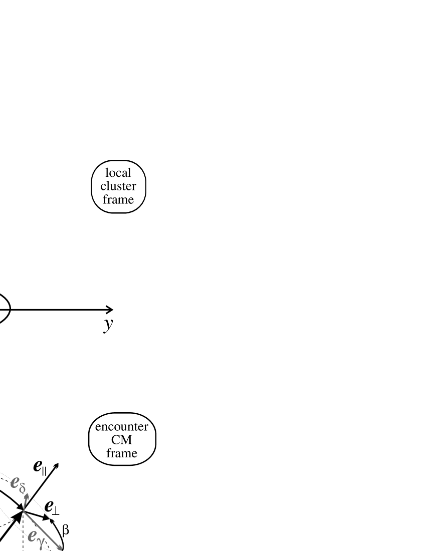
Figure 15: The reference frames used in the computation of the 2-body encounter. $\@vec{v}_{1,2}$ are the velocities of the stars in the local cluster frame, $\@vec{w}_{1,2}$, their velocities in the encounter reference frame, $\@vec{v}_{\mathrm{rel}}=\@vec{v}_{1}-\@vec{v}_{2}$ is the relative velocity and $\@vec{v}_{\mathrm{CM}}$ the velocity of their centre-of-mass (CM) in the cluster frame. See text for more details.

In this appendix, we detail the vectorial operations corresponding to steps 2, 3, and 4 of an individual encounter between two neighbouring super-stars, as described in Sect. 4.2.1.

Step 2. The situation is depicted on top of Fig. 15. A local reference frame, at rest in the cluster, is defined with axis $\mathrm{O}z$ pointing in the radial direction from the cluster’s centre and $\@vec{v}_{1}\in\mathrm{O}xz$. From the specific angular momenta $J_{i}$, kinetic energies $T_{i}$ and distances to centre $R_{i}$ of the super-stars, the moduli of the radial and tangential components of the stars’ velocities are deduced:

$$v_{i}^{\mathrm{tg}}=J_{i}/R_{i}\mbox{,\ \ }v_{i}^{\mathrm{rad}}=\sqrt{2T_{i}-(v_{i}^{\mathrm{tg}})^{2}}.$$ (32)

We set $v_{1}^{x}=v_{1}^{\mathrm{tg}}$, $v_{1}^{y}=0$ and $v_{1}^{z}=v_{1}^{\mathrm{rad}}$, $v_{2}^{x}=v_{2}^{\mathrm{tg}}\cos(\varphi_{2})$, $v_{2}^{y}=v_{2}^{\mathrm{tg}}\sin(\varphi_{2})$ and $v_{2}^{z}=\pm v_{2}^{\mathrm{rad}}$, with a random value for the angle $\varphi_{2}$ ($\in[0,2\pi]$) and the sign of $v_{2}^{z}$. This procedure accounts for the freedom in the relative orientation of $\@vec{v}_{1}$ and $\@vec{v}_{2}$, thus ensuring a correct sampling of the encounters’ incoming velocities.

Step 3. We now switch to the encounter CM reference frame (see bottom panel of Fig. 15) which has the same axis orientation as the cluster frame but translates with velocity $\@vec{v}_{\mathrm{CM}}=\lambda_{1}\@vec{v}_{1}+\lambda_{2}\@vec{v}_{2}$ ($\lambda_{i}=M_{i}/(M_{1}+M_{2})$ where $M_{1,2}$ are the masses of the stars). We use the notation $\@vec{v}_{1,2}$ for the stars’ velocities in the cluster frame and $\@vec{w}_{1,2}$ when we express them in the encounter frame. Prime (^′) denotes quantities after the encounter. We build an orthonormal vector set $\{\@vec{e}_{\parallel},\@vec{e}_{\gamma},\@vec{e}_{\delta}\}$ with $\@vec{e}_{\parallel}=\@vec{v}_{\mathrm{rel}}/v_{\mathrm{rel}}$ and $\@vec{e}_{\gamma},\@vec{e}_{\delta}\perp\@vec{v}_{\mathrm{rel}}$. The orientation of the orbital plane spanned by $\{\@vec{e}_{\parallel},\@vec{e}_{\perp}\}$ is set through a randomly chosen angle $\beta$ defining $\@vec{e}_{\perp}=\cos(\beta)\@vec{e}_{\gamma}+\sin(\beta)\@vec{e}_{\delta}$. In this frame, the effect of the gravitational encounter is simply to rotate the initial velocities (at infinity) $\@vec{w}_{1}=\lambda_{2}\@vec{v}_{\mathrm{rel}}$ and $\@vec{w}_{2}=-\lambda_{1}\@vec{v}_{\mathrm{rel}}$ by an angle $\theta_{\mathrm{SE}}$, so:

$$\begin{array}[]{l}\@vec{w}_{1}^{\prime}=\lambda_{2}\@vec{v}_{\mathrm{rel}}^{\prime}\mbox{,\ \ }\@vec{w}_{2}^{\prime}=-\lambda_{1}\@vec{v}_{\mathrm{rel}}^{\prime}\\ \mbox{with\ \ }\@vec{v}_{\mathrm{rel}}^{\prime}=v_{\mathrm{rel}}\left(\cos(\theta_{\mathrm{SE}})\@vec{e}_{\parallel}+\sin(\theta_{\mathrm{SE}})\@vec{e}_{\perp}\right).\end{array}$$ (33)

Step 4. Finally, the relevant post-encounter properties of the super-stars in the cluster frame are given by straightforward formulae:

$$T_{i}^{\prime} = \frac{1}{2}(\@vec{v}_{i}^{\prime})^{2},$$ (34)

$$J_{i}^{\prime} = R_{i}\sqrt{(v_{i}^{x\prime})^{2}+(v_{i}^{y\prime})^{2}}$$ (35)

with $\@vec{v}_{i}^{\prime}=\@vec{w}_{i}^{\prime}+\@vec{v}_{\mathrm{CM}}$.

Appendix B Random selection of a new orbital radius

Figure 16: Diagram of the random selection of an orbital position using a rejection method with a Keplerian comparison function. A constant $P_{\mathrm{selec}}(R)$ is assumed.

Figure 17: Example of the shape of the probability density $f_{\mathrm{plac}}\propto P_{\mathrm{selec}}(R)/v_{\mathrm{rad}}(R)$ for placing a super-star on its orbit. Hénon’s $s$ variable has been used instead of $R$ to remove the divergences of $v_{\mathrm{rad}}^{-1}$ at peri- and apo-centre ($R=R_{\mathrm{p}}+(R_{\mathrm{a}}-R_{\mathrm{p}})s^{2}(3-2s)$). $f_{\mathrm{plac}}$ is shown in solid line along with the simple Keplerian upper bound $P_{\mathrm{selec}}(R_{\mathrm{p}})/v_{\mathrm{rad}}^{(\mathrm{Kep})}(R)$ (dot-dashed line) and a refined Keplerian upper bound (dashes) with coarse account for the important radial decrease of $P_{\mathrm{selec}}$. $P_{\mathrm{selec}}$ was computed with the second method described in Sect. 4.2.2 where $T_{\mathrm{rel}}^{-1}$ is evaluated on a coarse rank grid. This is responsible for the saw tooth shape of $f_{\mathrm{plac}}$. Obviously, the “raw” Keplerian $f_{\mathrm{comp}}$ would mostly generate $R$ values near the apo-centre very likely to be rejected due to the actual very low probability density for such $R$s.

Here, we explain how we determine a new radius $R$ for a super-star after it has experienced a super-encounter (see Sect. 5.2).

Our goal is to generate random $R$ values whose distribution density comply with Eq. 30. The main difficulty lies in the fact that $f_{\mathrm{plac}}(R)$ is not an easily computable function. First, $P_{\mathrm{selec}}$ really depends on the rank rather than on $R$ and has generally no simple analytical expression (see Sect. 4.2.2). Furthermore, $v_{\mathrm{rad}}(R)$ is a function of $\Phi(R)$ which is not known analytically either. Obtaining the value of the rank or the potential (through local $A$ and $B$ coefficients) at any given $R$ implies a tree traversal. Given these intricacies, we don’t even attempt transforming a uniform-deviate random variable through the inverse function of the cumulative probability and turn to a rejection method (Press et al. 1992, Sect.7.3). The trick is to find a comparison function $f_{\mathrm{comp}}$, a more docile probability density which can be made a uniform upper bound to $f_{\mathrm{plac}}(R)$ ($f_{\mathrm{comp}}(R)\geq\alpha f_{\mathrm{plac}}(R)\;\forall R\in[R_{\mathrm{p}},R_{\mathrm{a}}]$ for some constant $\alpha$). We then proceed by generating a random number $R_{\mathrm{rand}}$ according to $f_{\mathrm{comp}}$ and another, $X_{\mathrm{rand}}$, with uniform deviation between 0 and 1. If $X_{\mathrm{rand}}\leq\alpha f_{\mathrm{plac}}(R_{\mathrm{rand}})/f_{\mathrm{comp}}(R_{\mathrm{rand}})$, $R_{\mathrm{rand}}$ is kept, otherwise it is rejected and we try again. The accepted $R_{\mathrm{rand}}$ values follow the $f_{\mathrm{plac}}$ distribution. Of course the closer the comparison function is to $f_{\mathrm{plac}}(R)$, the fewer rejection steps and the more efficient is the method (remember that a tree traversal is realised for each $f_{\mathrm{plac}}(R)$ evaluation).

By construction, $P_{\mathrm{selec}}$ is constrained to decrease with rank/radius, so an easy but inefficient upper bound is its value at peri-centre. As for $v_{\mathrm{rad}}(R)^{-1}$, we first applied Hénon’s variable change ($R=R_{\mathrm{p}}+(R_{\mathrm{a}}-R_{\mathrm{p}})s^{2}(3-2s)$) to remove the divergences at peri- and apo-centre but failed to find a safe upper bound for the resulting probability density of $s$. We instead use the fact that a shifted Keplerian potential $\Phi_{\mathrm{Kep}}(R)=C_{1}/R+C_{2}$ equal to $\Phi$ at $R_{\mathrm{p}}$ and $R_{\mathrm{a}}$ is everywhere higher (or equal) in between, so that

$$\frac{1}{v_{\mathrm{rad}}(R)} \leq \frac{1}{v_{\mathrm{rad}}^{(\mathrm{Kep})}(R)}=$$ (36)

$$\frac{\sqrt{R_{\mathrm{p}}R_{\mathrm{a}}}}{2J}\frac{R}{\sqrt{\left(R-R_{\mathrm{p}}\right)\left(R_{\mathrm{a}}-R\right)}}.$$

Furthermore, the cumulative probability function for this Keplerian bound is analytical:

$$F_{\mathrm{Kep}}(R) \propto \int_{R\mathrm{p}}^{R}\frac{r\,\mathrm{d}r}{\sqrt{\left(r-R_{\mathrm{p}}\right)\left(R_{\mathrm{a}}-r\right)}}$$ (37)

$$= \frac{2}{\pi}\left[\arctan\sqrt{\frac{x}{1-x}}-e\sqrt{x(1-x)}\right]$$

$$\mbox{with\leavevmode\nobreak\ \leavevmode\nobreak\ }x=\frac{R-R\mathrm{p}}{R\mathrm{a}-R\mathrm{p}}\mbox{\leavevmode\nobreak\ \leavevmode\nobreak\ and\leavevmode\nobreak\ \leavevmode\nobreak\ }e=\frac{R\mathrm{a}-R\mathrm{p}}{R\mathrm{a}+R\mathrm{p}}$$ .

So, to summarize, the selection of a new orbital radius proceeds as follows (see Fig. 16):

1. Generate a random number $X_{\mathrm{rand}}$ with $[0,1]$-uniform deviate.

2. Compute $R_{\mathrm{rand}}=R_{\mathrm{p}}+(R\mathrm{a}-R\mathrm{p})F^{-1}_{\mathrm{Kep}}(X_{\mathrm{rand}})$ using, for instance, Newton-Raphson algorithm.

3. Keep $R=R_{\mathrm{rand}}$ with probability

   $$P_{\mathrm{keep}}=\frac{P_{\mathrm{selec}}(R)}{P_{\mathrm{selec}}(R_{\mathrm{p}})}\frac{v_{\mathrm{rad}}^{(\mathrm{Kep})}(R)}{v_{\mathrm{rad}}(R)}.$$

This procedure actually had to be improved, for $P_{\mathrm{selec}}$ is generally very rapidly decreasing with rank. As a result, if the super-star’s orbit spans a large $R$-range, a constant bound often proves to be highly inefficient, requiring hundreds of rejection steps. So, when the number of unsuccessful tries reaches a limiting value, the $[R_{\mathrm{p}},R_{\mathrm{a}}]$ interval is sliced into a few sub-intervals and a stepped bound on $P_{\mathrm{selec}}$ is devised by computing its value at the lower rank of each sub-interval. Hence a comparison function is obtained that lies closer to $f_{\mathrm{plac}}$. However, in case a large number of rejections still fails to select a $R$ value, further successive refining is realized, using more and more sub-intervals to get closer and closer upper bounds to $P_{\mathrm{selec}}$. In practice, we use successively 5, 20 and 50 sub-intervals when the number of unsuccessful rejection cycles exceeds 10, 100 and 1000 respectively. This modification clearly complicates the computation of $F_{\mathrm{Kep}}$ and its inversion during phase 2. It appears as a numerical overhead as it imposes a tree traversals to determine lower rank values for each sub-interval. However, such added intricacies allow to break off from a (nearly) never ending rejection cycle. The improvement on the Keplerian comparison function is depicted for a typical case in Fig. 17. With this method, the average number of rejection cycles to attribute a new $R$ to a super-star lies between 5 and 10 in our cluster simulations.

Appendix C Binary tree structure and algorithms

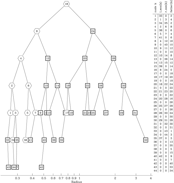
Figure 18: Binary tree structure containing 32 Super-stars (squares). 12 Super-stars have been evolved, leaving empty nodes (hexagons). In this diagram, the horizontal position of a node reflects the radius of the associated super-star. The logical structure of this tree is stored in the arrays whose content is displayed on the right.

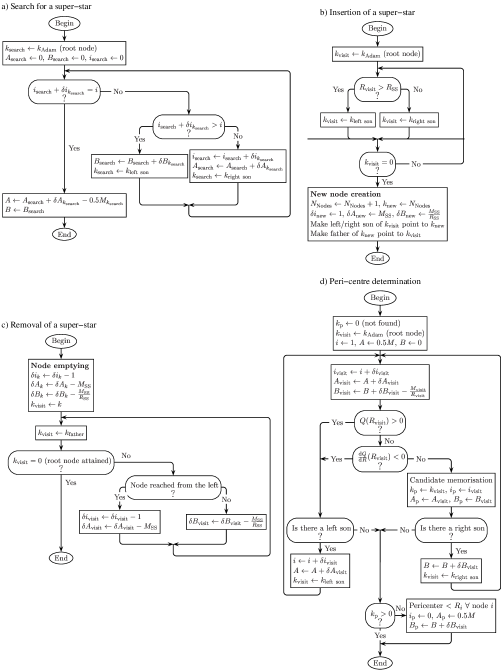
Figure 19: Flow charts for elementary binary tree routines. a) Search for super-star with rank $i$; on exit $A$ and $B$ are its potential coefficients (see Sect. 5.1). b) Insertion of a super-star of mass $M_{\mathrm{SS}}$ at radius $R_{\mathrm{SS}}$. c) Extraction of the super-star attached to node $k$. d) Peri-centre determination for a super-star of mass $M$. See text for the definition of $Q(R)$. On exit, $k_{\mathrm{p}}$ is the number of the last node with radius smaller than the peri-centre radius (in order of increasing radius), $i_{\mathrm{p}}$ the corresponding rank and $A_{\mathrm{p}}$, $B_{\mathrm{p}}$, the potential coefficients at peri-centre.

In this appendix, we present in some detail the implementation of the binary tree in charge of storing the potential and ranking information of the super-star cluster.

The logical structure of the tree is implemented by three integer arrays: l_son, r_son and father. l_son(k) is the number of the “left son” node of node k and so on, see Fig. 18. When the tree is (re-)built, each node k is attributed a super-star super_star(k). When this particle is evolved and moved to another radius, the node becomes empty and another leaf node is added to host the super-star. Leaving empty nodes simplifies the tree update procedures with the cost of increasing its size. This introduces some numerical overhead as it causes a faster increase of the number of hierarchical levels (particularly in the central regions where the time steps are shorter, see Fig. 18) but this inconvenience is probably not a serious concern for the tree is rebuilt from scratch from time to time in order to keep it reasonably well balanced. This operation is computationally cheap compared to the numerous tree traversals and would be called for even if empty nodes were not created.

To find a super-star with rank $i$ and compute the potential at its position, one traverses the tree from the root to the corresponding node using the algorithm sketched in Fig. 19a. At the end of this tree traversal, $k_{\mathrm{search}}$ points to the proper node and the super-star’s potential is $\Phi=-A/R_{k_{\mathrm{search}}}-B$. A very similar routine is used to compute the potential $\Phi(R)$ at any arbitrary radius $R$. Flow charts for addition/removal of a super-star into/from the binary tree are depicted in Fig. 19b, c.

Another important role of the binary tree is the computation of peri- and apo-centre radii for a given super-star, an obvious prerequisite to the radial placing procedure described in Sect. 5.2. Note that a high level of precision is called for: unphysical cluster evolution could expectedly arise if super-stars’ orbits suffered from any systematic bias. For lack of explicit knowledge of $\Phi(R)$, solving Eq. 26 is not straightforward. The main operation, depicted in Fig. 19d, is a tree traversal in a search for the node $k_{p}$ whose radius lies immediately below the peri-centre, i.e. with $Q(R)=v_{\mathrm{rad}}^{2}(R)<0$ and $\mathrm{d}Q/\mathrm{d}R>0$. This provides us with the local $A_{\mathrm{p}}$ and $B_{\mathrm{p}}$ potential coefficients. Hence, computing $R_{\mathrm{p}}$ reduces to the solution of the simple equation:

$$v_{\mathrm{rad}}^{2}=2E+2\frac{A_{\mathrm{p}}+0.5M}{R}+2B_{\mathrm{p}}+\frac{J^{2}}{R^{2}}=0.$$ (38)

Needless to say, the computation of the apo-centre radius is very similar.

Appendix D Tests for spurious relaxation

Figure 20: Tests for spurious relaxation in Plummer models with 4000 (left) and 64 000 (right) super-stars. Relaxation was switched off. The top panels show the evolution (or absence thereof) of Lagrangian radii. The bottom panels present the evolution of central properties: density ($\rho$), potential ($\Phi$) and velocity dispersion ($\sigma$). These quantities have been normalized by the average of the 20 first values of each sequence and the curves have been smoothed for the sake of clarity. Note that for $N_{\mathrm{SS}}=4000$, some spurious evolution happens while it is nearly suppressed for $N_{\mathrm{SS}}=64\,000$.

To measure the amplitude of the spurious relaxation due to the fact that we represent a smooth potential $\Phi$ by a set of super-stars, i.e. of spherical shells with zero thickness, we carried out a few simulations in which relaxation was switched off. In such cases, the algorithm reduces to moving the super-stars on their orbits again and again. Ideally, the structure of the cluster should not display any evolution but statistical fluctuations. Figure. 20 shows the results of such tests realized with 4000 and 64 000 particles. The computations where stopped when the total number of steps divided by the number of super-stars reached 4000. For comparison, our core-collapse simulation for a Plummer model with $2\times 10^{6}$ particles (Sect. 7.2) required an average of 2300 steps per super-star. From these relaxation-free tests, we conclude that the amount of spurious relaxation is negligible if the number of super-stars is of order 16 000 or larger.

References

- Aarseth & Heggie (1998) Aarseth, S. J. & Heggie, D. C. 1998, MNRAS, 297, 794
- Alexander (1999) Alexander, T. 1999, ApJ, 527, 835
- Arabadjis (1997) Arabadjis, J. S. 1997, PhD thesis, University of Michigan
- Armitage et al. (1996) Armitage, P. J., Zurek, W. H., & Davies, M. B. 1996, ApJ, 470, 237
- Bahcall & Wolf (1976) Bahcall, J. N. & Wolf, R. A. 1976, ApJ, 209, 214
- Bailey (1980) Bailey, M. E. 1980, MNRAS, 191, 195
- Baumgardt (2000) Baumgardt, H. 2000, Scaling of -body calculations, preprint, astro-ph/0012330
- Begelman et al. (1980) Begelman, M. C., Blandford, R. D., & Rees, M. J. 1980, Nat, 287, 307
- Benz (1990) Benz, W. 1990, in Numerical Modelling of Nonlinear Stellar Pulsations Problems and Prospects, ed. J. R. Buchler, 269–288
- Benz & Hills (1992) Benz, W. & Hills, J. G. 1992, ApJ, 389, 546
- Bettwieser & Sugimoto (1984) Bettwieser, E. & Sugimoto, D. 1984, MNRAS, 208, 493
- Bettwieser & Sugimoto (1985) —. 1985, MNRAS, 212, 189
- Binney & Tremaine (1987) Binney, J. & Tremaine, S. 1987, Galactic Dynamics (Princeton University Press)
- Boily (2000) Boily, C. M. 2000, in ASP Conf. Ser. 211: Massive Stellar Clusters, ed. A. Lançon & C. M. Boily, 190
- Cipollina & Bertin (1994) Cipollina, M. & Bertin, G. 1994, A&A, 288, 43
- Cohn (1979) Cohn, H. 1979, ApJ, 234, 1036
- Cohn (1980) —. 1980, ApJ, 242, 765
- Cohn & Kulsrud (1978) Cohn, H. & Kulsrud, R. M. 1978, ApJ, 226, 1087
- Danzmann (1996) Danzmann, K. 1996, Classical Quantum Gravity, 13, A247
- David et al. (1987a) David, L. P., Durisen, R. H., & Cohn, H. N. 1987a, ApJ, 313, 556
- David et al. (1987b) —. 1987b, ApJ, 316, 505
- Davies et al. (1998) Davies, M. B., Blackwell, R., Bailey, V. C., & Sigurdsson, S. 1998, MNRAS, 301, 745
- de Zeeuw (2001) de Zeeuw, T. 2001, in Black Holes in Binaries and Galactic Nuclei, Proceedings of the ESO Workshop held at Garching, Germany, 6-8 September 1999., ESO Astrophysics Symposia (Springer), 78
- Dokuchaev & Ozernoi (1977a) Dokuchaev, V. I. & Ozernoi, L. M. 1977a, Soviet Astronomy Letters, 3, 112
- Dokuchaev & Ozernoi (1977b) —. 1977b, Soviet Astronomy Letters, 3, 157
- Drukier et al. (1999) Drukier, G. A., Cohn, H. N., Lugger, P. M., & Yong, H. 1999, ApJ, 518, 233
- Eckart & Genzel (1996) Eckart, A. & Genzel, R. 1996, Nat, 383, 415
- Eckart & Genzel (1997) —. 1997, MNRAS, 284, 576
- Einsel (1998) Einsel, C. 1998, in Dynamics of Galaxies and Galactic Nuclei, An International Workshop of the SFB 328 Evolution of Galaxies held at the ITA November 03 - 05, 1997, ed. W. J. Duschl & C. Einsel, 31
- Einsel & Spurzem (1999) Einsel, C. & Spurzem, R. 1999, MNRAS, 302, 81
- Ford et al. (1998) Ford, H. C., Tsvetanov, Z. I., Ferrarese, L., & Jaffe, W. 1998, in IAU Symp. 184: The Central Regions of the Galaxy and Galaxies, ed. Y. Sofue, Vol. 184, 377
- Freitag (2000) Freitag, M. 2000, PhD thesis, Université de Genève
- Freitag (2001) —. 2001, Monte Carlo cluster simulations to determine the rate of compact star inspiraling to a central galactic black hole, to be published in the proceedings of the 3rd LISA Symposium
- Freitag & Benz (2001a) Freitag, M. & Benz, W. 2001a, A Comprehensive Set of Simulations of Collisions Between Main Sequence Stars in Galactic Nuclei, in preparation
- Freitag & Benz (2001b) —. 2001b, Monte Carlo Simulations of Dense Galactic Nuclei, to be published in: Deiters S., Fuchs B., Just R. and Spurzem R. (eds.) Dynamics of Star Clusters and the Milky Way (ASP Conf. Ser.), astro-ph/0101183
- Freitag & Benz (2001c) Freitag, M. & Benz, W. 2001c, in Black Holes in Binaries and Galactic Nuclei, Proceedings of the ESO Workshop held at Garching, Germany, 6-8 September 1999., ed. L. Kaper, E. P. J. van den Heuvel, & P. A. Woudt, ESO Astrophysics Symposia (Springer), 269–272
- Freitag & Benz (2001d) —. 2001d, A New Monte Carlo Code for Star Cluster Simulations: II. Central Black Hole and Stellar Collisions, in preparation
- Fukushige & Heggie (2000) Fukushige, T. & Heggie, D. C. 2000, MNRAS, 318, 753
- Gebhardt et al. (2000) Gebhardt, K., Pryor, C., O’Connell, R. D., Williams, T. B., & Hesser, J. E. 2000, AJ, 119, 1268
- Genzel et al. (1997) Genzel, R., Eckart, A., Ott, T., & Eisenhauer, F. 1997, MNRAS, 291, 219
- Genzel et al. (1994) Genzel, R., Hollenbach, D., & Townes, C. H. 1994, Reports of Progress in Physics, 57, 417
- Genzel et al. (2000) Genzel, R., Pichon, C., Eckart, A., Gerhard, O. E., & Ott, T. 2000, MNRAS, 317, 348
- Genzel et al. (1996) Genzel, R., Thatte, N., Krabbe, A., Kroker, H., & Tacconi-Garman, L. E. 1996, ApJ, 472, 153
- Gerhard (1994) Gerhard, O. E. 1994, in NATO Advanced Research Workshop on The Nuclei of Normal Galaxies - Lessons from the Galactic Center, ed. R. Genzel & A. I. Harris, 267–282
- Ghez et al. (1998) Ghez, A. M., Klein, B. L., Morris, M., & Becklin, E. E. 1998, ApJ, 509, 678
- Ghez et al. (1999a) Ghez, A. M., Morris, M., & Becklin, E. E. 1999a, in ASP Conf. Ser. 182: Galaxy Dynamics - A Rutgers Symposium, ed. D. R. Merritt, M. Valluri, & J. A. Sellwood, 24
- Ghez et al. (1999b) Ghez, A. M., Morris, M., & Becklin, E. E. 1999b, in ASP Conf. Ser. 186: The Central Parsecs of the Galaxy, ed. H. Falcke, A. Cotera, W. J. Duschl, F. Melia, & M. Rieke, 18
- Giersz (1998) Giersz, M. 1998, MNRAS, 298, 1239
- Giersz (2000a) —. 2000a, Monte Carlo Simulations of Star Clusters, preprint, astro-ph/006438
- Giersz (2000b) —. 2000b, Monte Carlo simulations of star clusters - II. Tidally limited, multi-mass systems with stellar evolution, preprint, astro-ph/0009341
- Giersz & Heggie (1994a) Giersz, M. & Heggie, D. C. 1994a, MNRAS, 268, 257
- Giersz & Heggie (1994b) —. 1994b, MNRAS, 270, 298
- Giersz & Heggie (1996) —. 1996, MNRAS, 279, 1037
- Giersz & Spurzem (1994) Giersz, M. & Spurzem, R. 1994, MNRAS, 269, 241
- Giersz & Spurzem (2000) —. 2000, MNRAS, 317, 581
- Goodman (1989) Goodman, J. 1989, in Dynamics of Dense Stellar Systems, ed. D. Merritt, 183–193
- Goodman & Hut (1993) Goodman, J. & Hut, P. 1993, ApJ, 403, 271
- Gould & Rix (2000) Gould, A. & Rix, H. 2000, ApJ Lett., 532, 29
- Hameury et al. (1994) Hameury, J.-M., King, A. R., Lasota, J.-P., & Auvergne, M. 1994, A&A, 292, 404
- Heggie (1994) Heggie, D. C. 1994, in Astrophysics with Special Purpose Computers, Tokyo University, 115
- Heggie (1997) Heggie, D. C. 1997, Star Cluster Simulations, preprint, astro-ph/9711185, To appear in: New Horizon of Computational Science, T. Ebisuzaki (ed.), Kluwer
- Heggie (2000) —. 2000, Mass Loss from Globular Clusters, preprint, astro-ph/0007336
- Heggie et al. (1999) Heggie, D. C., Giersz, M., Spurzem, R., & Takahashi, K. 1999, Highlights in Astronomy, 11, 591
- Heggie & Mathieu (1986) Heggie, D. C. & Mathieu, R. D. 1986, in The Use of Supercomputers in Stellar Dynamics, ed. P. Hut & S. L. W. McMillan, 233
- Heggie & Stevenson (1988) Heggie, D. C. & Stevenson, D. 1988, MNRAS, 230, 223
- Hénon (1960) Hénon, M. 1960, Annales d’Astrophysique, 23, 668
- Hénon (1966) Hénon, M. 1966, Comptes rendus des séances de l’Académie des Sciences, 262, 666
- Hénon (1971a) Hénon, M. 1971a, Ap&SS, 14, 151
- Hénon (1971b) —. 1971b, Ap&SS, 13, 284
- Hénon (1973) Hénon, M. 1973, in Dynamical structure and evolution of stellar systems, Lectures of the 3rd Advanced Course of the Swiss Society for Astronomy and Astrophysics (SSAA), ed. L. Martinet & M. Mayor, 183–260
- Hénon (1975) Hénon, M. 1975, in IAU Symp. 69: Dynamics of Stellar Systems, ed. A. Hayli, 133
- Hensler et al. (1995) Hensler, G., Spurzem, R., Burkert, A., & Trassl, E. 1995, A&A, 303, 299
- Hernquist et al. (1991) Hernquist, L., Hut, P., & Kormendy, J. 1991, Nat, 354, 376
- Ho (1999) Ho, L. C. 1999, in Observational Evidence for the Black Holes in the Universe, ed. S. K. Chakrabarti, 157
- Hut et al. (1992) Hut, P., McMillan, S., Goodman, J., Mateo, M., Phinney, E. S., Pryor, C., Richer, H. B., Verbunt, F., & Weinberg, M. 1992, PASP, 104, 981
- Inagaki & Saslaw (1985) Inagaki, S. & Saslaw, W. C. 1985, ApJ, 292, 339
- Inagaki & Wiyanto (1984) Inagaki, S. & Wiyanto, P. 1984, PASJ, 36, 391
- Jernigan & Porter (1989) Jernigan, J. G. & Porter, D. H. 1989, ApJS, 71, 871
- Joshi et al. (2001) Joshi, K. J., Nave, C. P., & Rasio, F. A. 2001, ApJ, 550, 691
- Joshi et al. (2000) Joshi, K. J., Rasio, F. A., & Portegies Zwart, S. 2000, ApJ, 540, 969
- Kim & Lee (1999) Kim, S. S. & Lee, H. M. 1999, A&A, 347, 123
- Knuth (1973) Knuth, D. E. 1973, The Art of Computer Programming, Volume 3, Sorting and Searching (Addison-Wesley)
- Kormendy & Richstone (1995) Kormendy, J. & Richstone, D. 1995, ARA&A, 33, 581
- Lai et al. (1993) Lai, D., Rasio, F. A., & Shapiro, S. L. 1993, ApJ, 412, 593
- Larson (1970a) Larson, R. B. 1970a, MNRAS, 150, 93
- Larson (1970b) —. 1970b, MNRAS, 147, 323
- Lauer et al. (1998) Lauer, T. R., Faber, S. M., Ajhar, E. A., Grillmair, C. J., & Scowen, P. A. 1998, AJ, 116, 2263
- Lee (1987) Lee, H. M. 1987, ApJ, 319, 801
- Lee (1995) —. 1995, MNRAS, 272, 605
- Lee et al. (1991) Lee, H. M., Fahlman, G. G., & Richer, H. B. 1991, ApJ, 366, 455
- Lee & Nelson (1988) Lee, H. M. & Nelson, L. A. 1988, ApJ, 334, 688
- Lee (1993) Lee, M. H. 1993, ApJ, 418, 147
- Lee & Goodman (1989) Lee, M. H. & Goodman, J. 1989, ApJ, 343, 594
- Leeuwin & Athanassoula (2000) Leeuwin, F. & Athanassoula, E. 2000, MNRAS, 317, 79
- Lightman & Shapiro (1977) Lightman, A. P. & Shapiro, S. L. 1977, ApJ, 211, 244
- Lin & Tremaine (1980) Lin, D. N. C. & Tremaine, S. 1980, ApJ, 242, 789
- Louis & Spurzem (1991) Louis, P. D. & Spurzem, R. 1991, MNRAS, 251, 408
- Lynden-Bell & Eggleton (1980) Lynden-Bell, D. & Eggleton, P. P. 1980, MNRAS, 191, 483
- Magorrian et al. (1998) Magorrian, J., Tremaine, S., Richstone, D., Bender, R., Bower, G., Dressler, A., Faber, S. M., Gebhardt, K., Green, R., Grillmair, C., Kormendy, J., & Lauer, T. 1998, AJ, 115, 2285
- Makino (1996) Makino, J. 1996, ApJ, 471, 796
- Makino (1997) —. 1997, ApJ, 478, 58
- Makino (1998) —. 1998, Highlights in Astronomy, 11, 597
- Makino (2000) —. 2000, Direct Simulation of Dense Stellar Systems with GRAPE-6, preprint, astro-ph/0007084
- Maoz (1998) Maoz, E. 1998, ApJ Lett., 494, 181
- Marchant & Shapiro (1980) Marchant, A. B. & Shapiro, S. L. 1980, ApJ, 239, 685
- McMillan (1993) McMillan, S. L. W. 1993, in ASP Conf. Ser. 50: Structure and Dynamics of Globular Clusters, ed. S. G. Djorgovski & G. Meylan, 171
- McMillan & Aarseth (1993) McMillan, S. L. W. & Aarseth, S. J. 1993, ApJ, 414, 200
- Merrit et al. (2000) Merrit, D., Cruz, F., & Milosavljević, M. 2000, Dynamics of Black-Hole Nuclei, preprint, astro-ph/008497
- Meylan & Heggie (1997) Meylan, G. & Heggie, D. C. 1997, A&AR, 8, 1
- Miralda-Escudé & Gould (2000) Miralda-Escudé, J. & Gould, A. 2000, ApJ, 545, 847
- Murphy & Cohn (1988) Murphy, B. W. & Cohn, H. N. 1988, MNRAS, 232, 835
- Murphy et al. (1991) Murphy, B. W., Cohn, H. N., & Durisen, R. H. 1991, ApJ, 370, 60
- Norman & Scoville (1988) Norman, C. & Scoville, N. 1988, ApJ, 332, 124
- Novikov et al. (1992) Novikov, I. D., Pethick, C. J., & Polnarev, A. G. 1992, MNRAS, 255, 276
- Peebles (1972) Peebles, P. J. E. 1972, ApJ, 178, 371
- Portegies Zwart et al. (1998) Portegies Zwart, S. F., Hut, P., Makino, J., & McMillan, S. L. W. 1998, A&A, 337, 363
- Press et al. (1992) Press, W. H., Teukolsky, S. A., Vetterling, W. T., & Flannery, B. P. 1992, Numerical Recipies in FORTRAN (Cambridge University Press)
- Quinlan (1996) Quinlan, G. D. 1996, New Astronomy, 1, 255
- Quinlan & Hernquist (1997) Quinlan, G. D. & Hernquist, L. 1997, New Astronomy, 2, 533
- Quinlan et al. (1995) Quinlan, G. D., Hernquist, L., & Sigurdsson, S. 1995, ApJ, 440, 554
- Rasio (2000) Rasio, F. A. 2000, Monte Carlo Simulations of Globular Clusters Dynamics, preprint, astro-ph/0006205
- Rauch (1995) Rauch, K. P. 1995, MNRAS, 275, 628
- Rees (1988) Rees, M. J. 1988, Nat, 333, 523
- Rees (1990) —. 1990, Science, 247, 817
- Rees (1997) Rees, M. J. 1997, in Reviews of Modern Astronomy, Vol. 10, 179–190
- Saslaw (1985) Saslaw, W. C. 1985, Gravitational physics of stellar and galactic systems (Cambridge, Cambridge University Press)
- Sedgewick (1988) Sedgewick, R. 1988, Algorithms, Second Edition (Addison-Wesley)
- Shapiro (1985) Shapiro, S. L. 1985, in IAU Symp. 113: Dynamics of Star Clusters, ed. J. Goodman & P. Hut, 373–412
- Shapiro & Lightman (1976) Shapiro, S. L. & Lightman, A. P. 1976, Nat, 262, 743
- Shapiro & Marchant (1978) Shapiro, S. L. & Marchant, A. B. 1978, ApJ, 225, 603
- Sigurdsson et al. (1995) Sigurdsson, S., Hernquist, L., & Quinlan, G. D. 1995, ApJ, 446, 75
- Spitzer (1975) Spitzer, L. 1975, in IAU Symp. 69: Dynamics of Stellar Systems, ed. A. Hayli, 3
- Spitzer (1987) Spitzer, L. 1987, Dynamical evolution of globular clusters (Princeton University Press)
- Spitzer & Mathieu (1980) Spitzer, L. & Mathieu, R. D. 1980, ApJ, 241, 618
- Spitzer & Shull (1975a) Spitzer, L. & Shull, J. M. 1975a, ApJ, 200, 339
- Spitzer & Shull (1975b) —. 1975b, ApJ, 201, 773
- Spitzer (1969) Spitzer, L. J. 1969, ApJ Lett., 158, 139
- Spitzer & Hart (1971) Spitzer, L. J. & Hart, M. H. 1971, ApJ, 164, 399
- Spitzer & Thuan (1972) Spitzer, L. J. & Thuan, T. X. 1972, ApJ, 175, 31
- Spurzem (1999) Spurzem, R. 1999, Journal of Computational and Applied Mathematics, 109, 407
- Spurzem & Aarseth (1996) Spurzem, R. & Aarseth, S. J. 1996, MNRAS, 282, 19
- Spurzem & Einsel (1999) Spurzem, R. & Einsel, C. 1999, in ASP Conf. Ser. 182: Galaxy Dynamics - A Rutgers Symposium, ed. D. R. Merritt, M. Valluri, & J. A. Sellwood, 105
- Spurzem & Kugel (2000) Spurzem, R. & Kugel, A. 2000, in Molecular Dynamics on Parallel Computers, ed. R. Esser, P. Grassberger, J. Grotendorst, & M. Lewerenz (World Scientific), 264–275
- Spurzem & Takahashi (1995) Spurzem, R. & Takahashi, K. 1995, MNRAS, 272, 772
- Stodołkiewicz (1982) Stodołkiewicz, J. S. 1982, Acta Astron., 32, 63
- Stodołkiewicz (1986) —. 1986, Acta Astron., 36, 19
- Syer et al. (1991) Syer, D., Clarke, C. J., & Rees, M. J. 1991, MNRAS, 250, 505
- Taiji et al. (1996) Taiji, M., Makino, J., Fukushige, T., Ebisuzaki, T., & Sugimoto, D. 1996, in IAU Symp. 174: Dynamical Evolution of Star Clusters: Confrontation of Theory and Observations, ed. P. Hut & J. Makino, 141
- Takahashi (1993) Takahashi, K. 1993, PASJ, 45, 233
- Takahashi (1995) —. 1995, PASJ, 47, 561
- Takahashi (1996) —. 1996, PASJ, 48, 691
- Takahashi (1997) —. 1997, PASJ, 49, 547
- Takahashi & Portegies Zwart (1998) Takahashi, K. & Portegies Zwart, S. F. 1998, ApJ Lett., 503, 49
- Thorne (1998) Thorne, K. S. 1998, in Black Holes and Relativistic Stars, ed. R. M. Wald, 41
- van der Marel (1999) van der Marel, R. P. 1999, in IAU Symp. 186: Galaxy Interactions at Low and High Redshift, ed. J. E. Barnes & D. B. Sanders, Vol. 186, 333
- Voit & Shull (1988) Voit, G. M. & Shull, J. M. 1988, ApJ, 331, 197
- Vokrouhlický & Karas (1998a) Vokrouhlický, D. & Karas, V. 1998a, MNRAS, 293, L1
- Vokrouhlický & Karas (1998b) —. 1998b, MNRAS, 298, 53
- Watters et al. (2000) Watters, W. A., Joshi, K. J., & Rasio, F. A. 2000, ApJ, 539, 331
- Williams et al. (1999) Williams, R. J. R., Baker, A. C., & Perry, J. J. 1999, MNRAS, 310, 913
- Wirth (1976) Wirth, N. 1976, Algorithms + Data Structures = Programs (Prentice-Hall)
- Young (1980) Young, P. J. 1980, ApJ, 242, 1232