NICMOS Observations of Extragalactic Cepheids. I. Photometry Database and a Test of the Standard Extinction Law^†

Abstract

We present the results of near-infrared observations of extragalactic Cepheids made with the Near Infrared Camera and Multi-Object Spectrometer on board the Hubble Space Telescope. The variables are located in the galaxies IC 1613, IC 4182, M31, M81, M101, NGC 925, NGC 1365, NGC 2090, NGC 3198, NGC 3621, NGC 4496A and NGC 4536. All fields were observed in the F160W bandpass; additional images were obtained in the F110W and F205W filters. Photometry was performed using the DAOPHOT II/ALLSTAR package.

Self-consistent distance moduli and color excesses were obtained by fitting Period-Luminosity relations in the $H$, $I$ and $V$ bands. Our results support the assumption of a standard reddening law adopted by the HST Key Project on the Extragalactic Distance Scale. A companion paper will determine true distance moduli and explore the effects of metallicity on the Cepheid distance scale.

Subject headings: Cepheids — distance scale

1 Introduction

One of the most important legacies of the Hubble Space Telescope (HST) will undoubtedly be its revolutionary increase in the number of Cepheid-based distances to nearby galaxies. Two major projects, the HST Key Project on the Extragalactic Distance Scale (Freedman et al., 2001a) and the HST SN Ia Calibration Project (Saha et al., 1999), as well as smaller collaborations have resulted in the discovery of over 700 Cepheid variables and the determination of distances to 27 galaxies. This number will continue to grow as the community continues to take advantage of HST’s unparalleled ability to deliver high-resolution images of the crowded spiral arms where Cepheids are located. The next generation of instruments to be installed on board HST will increase its sensitivity and resolution and will extend these observations to larger distances.

Most HST Cepheid observations have concentrated on obtaining data in the $V$ band (typically in eight to thirteen non-aliasing epochs) with some additional $I$-band data, usually four to eight epochs. Although sparsely sampled, the $I$-band light curves are important for several reasons. First, they provide confirmation of the variables as Cepheids, since the $V$ and $I$ light curves should track each other, with the latter displaying an amplitude of about half of that of the former. Second, the $V-I$ colors should be consistent with those of Cepheids in the instability strip. Third, and most important, the $I$-band data provide the only means of correcting the observed distance modulus $\mu_{V}$ for extinction through the relation

$$\mu_{0}=\mu_{V}-{\cal R}_{V\!-\!I}\langle E(V\!-I)\rangle$$ (1)

where ${\cal R}_{V\!-\!I}=2.45$ is the adopted ratio of total-to-selective extinction for the $V$-band (Cardelli et al., 1989) and $\langle E(V\!-I)\rangle$ is the mean color excess of the Cepheid sample (§5 contains a calculation of the value of ${\cal R}_{V\!-\!I}$). This approach makes the true distance modulus quite sensitive to both ${\cal R}_{V\!-\!I}$ and $\langle E(V\!-I)\rangle$. A better procedure (Freedman & Madore, 1990) involves fitting a standard extinction curve through observed distance moduli at several wavelengths (usually $B$, $V$, $R$ and $I$) and extrapolating the fit to $\lambda^{-1}=0$. This approach is less susceptible to uncertainties in the individual observed distance moduli, and can also be used to test the assumed reddening law.

As the HST Key Project on the Extragalactic Distance Scale started its final cycle of observations, a subset of the team joined forces with colleagues outside the group to extend the work further into the infrared. Our aim was to perform random-phase near-IR photometry of a sample of Cepheids in fourteen galaxies and to combine the new and existing observed distance moduli. Such a data set would allow us to improve the derivation of true distance moduli, check the assumptions behind Equation (1), and perhaps explore the effects of metallicity on the Cepheid distance scale.

The paper is organized as follows: §2 describes the observations and the data reduction pipeline; §3 delineates the steps followed to obtain accurate and precise photometry in our fields; §4 presents the Cepheid sample, period-luminosity relations, and observed distance moduli; §5 discusses our results.

2 Observations and Data Reduction

2.1 Observations

The HST Near Infrared Camera and Multi-Object Spectrograph (NICMOS) instrument (Thompson, 1993), with its high spatial resolution and low thermal background, was uniquely suited to carry out the observations required by our program. NICMOS contains three cameras (named 1, 2 and 3) which illuminate Rockwell $256\times 256$ HgCdTe arrays. The cameras have different pixel scales (0$\farcs$043, 0$\farcs$076 and 0$\farcs$2, respectively), resulting in fields-of-view of 11″, 19″ and 51″, respectively. Since Cepheids are scattered throughout the spiral arms of the target galaxies, we chose Camera 2 (hereafter NIC2) as it provided the best trade-off between resolution and coverage.

The fourteen galaxies selected for this study are listed in Table 1. The selection of specific fields within each galaxy was based on known positions and periods of Cepheids, in order to maximize the number of variables and our coverage of the Period-Luminosity plane. We observed two fields in M101, matching those observed by Stetson et al. (1998) and Kelson et al. (1996). These will be hereafter referred to as “M101-Inner” and “M101-Outer.”

The observations followed the standard SPIRAL-DITH pattern, with two to four pointings depending on the field and filter used. Exposure times for each pointing ranged from 16s for M31 to 640s for the most distant galaxies. Some of the latter fields were imaged multiple times in order to increase measurement precision.

2.2 Data reduction

Once NICMOS had been installed on board HST, several instrument characteristics were discovered. One is a variable additive bias (called “pedestal”) introduced during array reset, which has a different amplitude in each of the four quadrants that make up the array. Because HgCdTe arrays do not have overscan regions, it is impossible to automatically remove this effect in the STScI pipeline. Therefore, the bias offset is modulated by the flat field and appears as an inverse flat-field pattern in the final image. A second characteristic of the detectors is a noiseless signal gradient (called “shading”), which is a temperature- and pixel- dependent bias that changes in the direction of pixel clocking during read-out. This presented a problem because the original implementation of the STScI processing pipeline did not use temperature-dependent darks. The combination of “pedestal” and “shading,” resulted in images with prominent spurious features. The level of photometric precision required by our program made it necessary to remove these instrumental effects. We did so by retrieving the raw frames from the STScI Archive and reprocessing them as described below.

Our reprocessing of the data was performed using the NICMOS pipeline present in IRAF/STSDAS with some modifications. First, temperature-dependent dark frames were generated and used when running the first part of the pipeline (a program called calnicA). This removed the “shading” effect.

The “pedestal” effect was corrected using a program outside of the standard pipeline, courtesy of R. van der Marel (STScI). The program read in an image created by calnicA, removed the flat-fielding imposed by it, and executed a loop to identify the pedestal. The pedestal is in fact measured by exploiting the property that a flat-fielded bias imparts fluctuations on the background of the final image. The fluctuations reach a minimum when the pedestal is removed completely. Once a robust minimum was found in each of the quadrants, the best-fit pedestals were removed. Lastly, the image was flat-fielded and written to disk.

Having obtained images with proper zero, dark and flat-field corrections, the second part of the pipeline ( calnicB) was run to combine the dithered pointings of each target field and produce a final mosaic. In addition, we used the dither package to produce higher-resolution mosaics of the M101 fields in the F160W band. This was possible thanks to the existence of four pointings per field in that galaxy.

3 Photometry

3.1 Technique

The mosaics were analyzed with the DAOPHOT II/ ALLSTAR software package (Stetson, 1994). Objects were detected with the FIND routine set to a threshold of $3\sigma$ above sky, and aperture photometry was carried out with the PHOT routine, using different apertures and sky annuli for each filter (see below for details). Point-spread functions were determined by the PSF routine for each field using bright, isolated stars present in the frame. After an initial ALLSTAR run, the star-subtracted frame was put through the FIND algorithm once more to pick up any additional $3\sigma$ objects. Object lists were merged and ALLSTAR was run one last time on the original image.

PSF magnitudes were brought onto a consistent aperture magnitude system using DAOGROW (see Stetson 1990 for details; only a short summary is presented here). Aperture photometry was obtained for PSF stars in each field ($\sim 450$ in total) using a monotonically increasing set of radii. DAOGROW then solved for a function representing the “growth curve”, i.e., the change in aperture magnitude as a function of radius. The cumulative growth curves for the F110W, F160W and F205W bands are shown in Figure 1. Other programs in the DAOPHOT suite used this information to transform PSF magnitudes to aperture magnitudes for objects of interest in each frame.

3.2 Absolute photometric calibrations

The NICMOS primary standards are G191-B2B, a white dwarf, and P330-E, a solar analog. These two stars provide absolute calibration in the white dwarf and solar analog scales, respectively. Since Cepheids have colors similar to those of solar analog stars, we used P330-E for the determination of magnitude zeropoints. We used NICMOS observations of G191-B2B, P330-E, and P117-D (another solar analog standard) for the determination of color terms. Ground-based $JHK$ photometry for NICMOS standards comes from Persson et al. (1998).

3.2.1 Magnitude zeropoints

Our definition of $J$, $H$ and $K$ zeropoints is based on different apertures and sky annuli for each band, to match the noticeable increase in FWHM as a function of wavelength. Table 2 lists our choices of aperture radius and inner and outer sky annuli for each of the three bandpasses. In the case of the drizzled M101 F160W images, which have twice the spatial resolution, all radii were increased by a factor of two in pixel units so they would subtend the same angular size.

Marcia Rieke kindly provided us with synthetic (TinyTim) stellar images as well as NICMOS observations of P330-E, which we used to derive the magnitude zeropoints for our choices of aperture and sky annuli. First, we computed the ratio of TinyTim counts to observed NICMOS count rates for P330-E as a function of aperture radius. We found this ratio to be constant, at the 0.05%, 0.03%, and 1.77% levels for F110W, F160W and F205W, respectively, over a large range in radius (5–25 pixels). This confirmed that the TinyTim image was a good representation of the actual system PSF.

We then re-scaled the TinyTim image (in arbitrary units) to match the actual mean observed count rate of P330-E; this produced a synthetic image of P330-E that could be used to perform aperture measurements on a “perfect” image free of defects, cosmic rays, or any other source of scatter found in real images. Next, we ran DAOPHOT’s PHOT routine on the synthetic P330-E images using the same aperture and sky annuli as for the Cepheid photometry. DAOPHOT quoted measurement errors of 0.004 mag for these magnitudes. Lastly, we combined the Persson et al. (1998) standard magnitudes and the DAOPHOT NICMOS instrumental magnitudes for P330-E to arrive at our magnitude zeropoints, listed in Table 2.

3.2.2 Color terms

Since the NICMOS filters are not exact matches to the standard filters, color term corrections had to be determined. Synthetic spectra of the NICMOS standards were created based on Kurucz’ latest solar-abundance models. These model spectra were convolved with two sets of transmission curves: one contained the NICMOS filter responses plus the quantum efficiency of camera 2, while the other was based on standard filter responses plus an atmospheric transmission curve. This allowed us to predict F110W, F160W, F205W, $J$, $H$ and $K$ magnitudes for the NICMOS standards. We then compared our results with published values (Persson et al., 1998) and found negligible offsets of $0.002\pm 0.003$ mag for $J$ and $H$ and a small offset of $0.022\pm 0.001$ mag for $K$.

We used the same model atmospheres and transmission curves described above to generate synthetic spectra for a variety of spectral types (F, G and K) and luminosity classes (I and V). We compared the values of $\langle F110W-J\rangle$ and $\langle F160W-H\rangle$ as a function of $\langle F110W-F160W\rangle$ as well as the values of $\langle F205W-K\rangle$ as a function of $\langle F160W-F205W\rangle$. We found

$$\langle F110W-J\rangle = 0.013\pm 0.006+$$

$$0.315 \pm 0.011\ \langle F110W-F160W\rangle$$ (2)

$$\langle F160W-H\rangle = 0.003\pm 0.002+$$

$$0.071 \pm 0.005\ \langle F110W-F160W\rangle$$ (3)

$$\langle F205W-K\rangle = 0.053\pm 0.008-$$

$$0.556 \pm 0.085\ \langle F160W-F205W\rangle$$ (4)

where $\langle F110W-F160W\rangle$ and $\langle F160W-F205W\rangle$ are the mean instrumental colors of the star to be corrected. These formulae are suitable for correcting our data since our F110W, F160W and F205W observations were taken within minutes of each other.

The mean values of the corrections were $0.23\pm 0.11$ mag for $\langle F110W-J\rangle$, $0.05\pm 0.02$ mag for $\langle F160W-H\rangle$ and $-0.04\pm 0.08$ mag for $\langle F205W-K\rangle$. Note that an exact correction for $\langle F160W-H\rangle$ was only applied to the stars in the IC 1613, M31, M101-Inner and M101-Outer fields. The other fields were observed only in F160W and therefore only an average H-band correction of $0.03$ mag could be applied, based on a mean Cepheid $\langle F110W-F160W\rangle$ color of $0.46$ mag.

3.3 Photometric recovery tests

The dense nature of most of our fields makes it difficult to obtain accurate values of the local sky around each object and to perform unbiased magnitude measurements. This effect is commonly referred to as “crowding”. In order to characterize its impact on our measurements, we injected artificial stars into each field and compared their input magnitudes with the recovered values. We used the point-spread functions derived for each field to generate the artificial stars, which were placed randomly across each field. The objects spanned a magnitude range including that encompassed by the variables. In the case of the M101 fields, we injected artificial stars into the original-resolution mosaics as well as the higher-resolution ones created by drizzling. We re-ran our photometry programs on the new images and searched the new star lists to locate the artificial stars.

The results of the tests are summarized in Table 3 and displayed in Figures 2a-b. Figure 2a contains plots of the difference between input and recovered magnitudes as a function of magnitude for each field. Figure 2b shows the strong correlation that exists between the crowding bias and the stellar density of each field. The effect ranges from 0.01 mag for the least crowded fields to 0.09 mag for the denser ones. All magnitudes were corrected for this effect.

In addition to these “crowding” tests, we also undertook simulations to estimate the contamination of Cepheid magnitudes by unresolved nearby stars. These “blending” tests are presented in §5.

3.4 Photometry checks

We performed several internal and external photometry checks to ensure the accuracy and precision of our magnitudes. We tested our aperture correction technique by comparing our corrected magnitudes against “standard” aperture magnitudes for stars in the IC 1613 fields. We found no significant difference ($<0.01$ mag) between the two sets. We also tested the repeatability of our PSF photometry by comparing magnitudes of objects that appeared twice in our data set, due to some overlap between different fields in M81 and M101. We found that the magnitude differences were consistent with the reported uncertainties.

We also performed an external photometry check by comparing HST and ground-based photometry of bright, isolated stars in our IC 1613 fields. The ground-based photometry was obtained at the Las Campanas 2.5-m du Pont telescope using its infrared camera (Persson et al., 1992) over fourteen nights between November 1993 and November 1996. Photometry was conducted using DAOPHOT II/ALLSTAR and DAOGROW (as described in §3.1) on 19 stars common to our ground-based and HST images. Table 4 lists their magnitudes and Figure 3 shows a comparison of the two systems; the mean offset is $0.011\pm 0.061$ mag, in the sense that the HST magnitudes are marginally brighter. Unfortunately, there was no published $J$- or $K$-band photometry available for stars in any of our fields, so we were unable to check our transformation of NICMOS F110W and F205W magnitudes.

4 The Cepheid sample

4.1 Sample selection and identification

As described in §2.1, we targeted specific fields within each galaxy in order to maximize the number of variables and our coverage of the Period-Luminosity plane. We selected the variables in each galaxy based on published catalogs, applying the following selection criteria: i) existence of both $V$ and $I$ photometry; ii) range in color of $0.5<V\!-\!I<1.75$; iii) periods between 10 days and the width of the observing window (applicable to Cepheids discovered with HST). Our fields contained 93 variables that met these criteria.

Cepheids in M31 and IC1613 were identified by visual inspection, using finding charts created from ground-based images. These fields are sparse enough that identifications did not present a problem, and twelve variables were located. In the case of the other galaxies, identifications followed a more rigorous process. First, the FITS header coordinates for the center of the mosaic were used to obtain a rough alignment and rotation relative to an optical image (from WFPC2 in most cases). Next, bright stars present in both the optical and the near-IR images were identified and used as input to the IRAF task geomap to determine the geometric transformations between the images. Lastly, the task geoxytran was used to predict the coordinates of 81 variables.

The DAOPHOT star lists generated in §3.1 were used to locate the object nearest to the predicted position of the variables. In general, counterparts were found within one pixel of their predicted location. Figure 4 shows the distribution of differences between the predicted and actual positions. Based on this figure, we decided to reject any candidate located more than 1.5 pixels (0$\farcs$11) away from its predicted position. This process resulted in the rejection of 11 possible counterparts.

In order to further discriminate between real counterparts and field contaminants, we plotted $V\!-\!H$ vs. $V\!-\!I$ colors for all remaining candidates (Figure 5a). The Cepheids follow a vector that is a combination of two closely degenerate quantities: the reddening trajectory and the color-color relation for these bands. Several objects deviate significantly from the rest of the sample; we suspect these are variables which are blended with unresolved red or blue companions. We performed a least-squares fit to the sample, using a fixed slope of $V\!-\!H/V\!-\!I=1.71$ (the average of the reddening and color-color slopes). The fit is shown in Fig. 5a as a solid line, while the dashed lines correspond to twice the r.m.s. deviation, or 0.46 mag. We rejected twelve possible counterparts that fell outside of the dashed boundaries.

Figure 5b shows a histogram of the deviations from the best-fit line. The asymmetric distribution of the outliers is to be expected, since we are more likely to detect a Cepheid that is blended with a red (i.e., IR-bright) field star than with a blue (i.e., IR-faint) one. Note that this color-color rejection process is insensitive to blends of Cepheids with stars of similar colors, a point to which we will return later.

In conclusion, our final sample consists of 70 variables (93 original candidates – 11 astrometric rejections – 12 color-color rejections). Finding charts for fields containing at least one variable are shown in Figures 6a-f, while Figures 7a-b contain close-up views of each object. Table 5 presents periods and magnitudes for the final Cepheid sample. We include in this Table the previously-published optical magnitudes of the variables. There are minor variations in the $V$ and $I$ zeropoints used in the different sources of optical photometry, reflecting the evolution in our knowledge of the HST calibration from 1994 to the present (see Mould et al. 2000 for details). For our target galaxies, the mean difference between the various calibrations used in the published papers and the current calibration (Stetson, 1998) amounts to $-0.03\pm 0.03$ mag in V, $-0.05\pm 0.04$ mag in I and $+0.02\pm 0.02$ mag in $V\!-\!I$.

4.2 Period-Luminosity relations

The method used to derive observed distance moduli is the same as that used by the HST Key Project on the Extragalactic Distance Scale (see Freedman et al., 2001a, for details). It is based on the Period-Luminosity relations of individually de-reddened LMC Cepheids from Udalski et al. (1999) ($V$ and $I$) and Persson et al. (2001) ($J$, $H$ and $K$), scaled to an assumed true distance modulus of $\mu_{0,{\rm LMC}}$ = 18.50$\pm$0.10 mag (total uncertainty). The relations are:

$$M_{V} = -2.76(\pm 0.03)\left[\log{\rm P}-1\right]-4.22(\pm 0.02),$$ (5)

$$M_{I} = -2.96(\pm 0.02)\left[\log{\rm P}-1\right]-4.90(\pm 0.01),$$ (6)

$$M_{H} = -3.23(\pm 0.04)\left[\log{\rm P}-1\right]-5.66(\pm 0.05),$$ (7)

$$M_{J} = -3.15(\pm 0.05)\left[\log{\rm P}-1\right]-5.32(\pm 0.06),$$ (8)

$$M_{K} = -3.26(\pm 0.04)\left[\log{\rm P}-1\right]-5.73(\pm 0.05).$$ (9)

In fitting the data from each field and filter, we fix the slope to the one given in the corresponding equation and obtain a magnitude shift by minimizing the unweighted rms dispersion. The resulting magnitude shifts are converted to observed distance moduli by subtracting the relevant magnitude zeropoint.

4.3 Observed distance moduli

Period-Luminosity relations were constructed for each field and filter using the data listed in Table 5 and fitted using Equations 5-9. Figures 8a-f show our near-IR P-L relations, while Figures 9a-e present the optical ones. In each panel, the solid line represents the results of the fitting process described in §4.2 while the dashed lines indicate the rms uncertainty of the fit. Fit results are displayed in each panel and listed in Tables 6 and 7.

We also tabulate in Table 6 published distance moduli for these galaxies (mostly from Table 4 of Freedman et al., 2001a), determined from substantially larger samples of variables and using the Stetson (1998) zeropoints. The optical distance moduli determined from our smaller samples should not take precedence over the above values. The optimum combination of the optical and infrared results will appear in Freedman et al. (2001b).

5 Blending effects in M101 Inner

As mentioned in the introduction, one of the motivations of this project was to further study the metallicity dependence of the Cepheid Period-Luminosity relation. Our data can contribute to these studies on two ways: first, a global test of the metallicity dependence can be performed by analyzing the apparent distance moduli of all galaxies; second, a differential test of the effect can be performed by analyzing the distance moduli to two regions of the same galaxy, provided they differ significantly in abundance. The first approach was undertaken by Kochanek (1997), while the second one was followed by Freedman & Madore (1990) in M31 and by Kennicutt et al. (1998) in M101. The differential test is a challenging one, because the Inner field of M101 deviates substantially from other Key Project fields in terms of surface brightness and stellar density.

Our near-infrared distance moduli to the inner and outer fields in M101 exhibit large differences: $\Delta\mu_{H}=0.46\pm 0.12$ mag and $\Delta\mu_{J}=0.37\pm 0.12$ mag. If taken at face value, they imply a very large metallicity dependence, of the order of 0.6 mag/dex. However, other observational effects could be contributing to the observed differences in distance moduli. One of them is “blending”, or the contamination of Cepheid fluxes by nearby stars, not physically associated with the variables, that fall within the NICMOS seeing disk and cannot be resolved. This effect has been the subject of a recent investigation in the optical by Mochejska et al. (2000).

One way to characterize the effect of blending on our distance determination to M101-Inner is to move nearby, well-resolved fields to the distance of M101, re-observe Cepheids in these fields, and compare the resulting magnitudes with the ones obtained from the original images. Our program contains observations of two suitable galaxies: M31 and M81. The fields observed in these galaxies show similar stellar densities and mean nearest-neighbor distances between Cepheids when compared to our M101-Inner fields. We used our two M81 fields as well as fourteen of our M31 fields, which were located in Fields I and III of Baade & Swope (1965).

We started by collecting the positions and magnitudes reported by ALLSTAR for all objects in our input fields. The separation between stars were reduced by the ratio of distances between the input galaxies and the M101-Outer field ($D(M101/M31)=10.1$ and $D(M101/M81)=2.2$). The input magnitudes were corrected for the exposure time of the original frames and distance to the input galaxies, and then modified to reflect the distance of M101 and the exposure time of the M101 frames. The stars were added to blank frames using the ADDSTAR routine found in DAOPHOT, which takes into account the properties of the detector and the PSF, as well as photon statistics. The artificial fields are shown in Figure 10 and compare favorably with the actual M101-Inner images shown in Figures 6a-f.

Once the artificial fields had been generated, they were photometered in exactly the same way as our real data. To identify the variables in our artificial frames, we used the input positions as the equivalent of the astrometric information available for the real data, and searched for the objects nearest to those positions, subject to the same 1.5-pixel rejection criterion from §4.1. All Cepheids that were recovered were located at distances smaller than the rejection limit.

Figure 11 shows the P-L relations obtained from the simulation, compared with the original input data. Seven long period Cepheids ($P>20$ d) exhibit changes in magnitude of order 0.1-0.2 mag, most of them being in the expected direction (i.e., towards brighter magnitudes). In the case of the eight Cepheids with short periods ($P<20$ d), one was not recovered, four exhibited large variations (which would have resulted in their rejection based on color-color criteria), and three had very modest changes in magnitude.

The resulting distance moduli are smaller than the input ones by 0-0.2 mag, depending on the period cutoff applied to these small samples. The rms scatter of the relations do not increase significantly, once the short-period outliers are removed from the fits. We therefore conclude that a substantial fraction of the difference in distance moduli between M101-Inner and M101-Outer could be due to blending. This prevents us from performing a differential determination of the metallicity effect; however, a global test can still be performed using the other galaxies we have observed.

6 Consistency of reddening determinations

Another goal of this project is to test whether the mean $V\!-\!I$ color excess, $\langle E(V\!-I)\rangle$, is an appropriate indicator of total extinction and whether it can be used to obtain true distance moduli. One could claim that the range in wavelength between these two bands is too small to allow a good extrapolation to $\lambda^{-1}=0$. There is also no guarantee that a “standard” value of ${\cal R}_{V\!-\!I}$ is applicable to other galaxies. If $\langle E(V\!-I)\rangle$ is indeed a good indicator of reddening, and if a standard reddening law (Cardelli et al., 1989) applies to other galaxies, then one would expect $\langle E(V\!-I)\rangle$ and $\langle E(V\!-H)\rangle$ to be strongly correlated and to follow the slope predicted by the standard reddening law.

6.1 Predicted relation between $\langle E(V\!-I)\rangle$ and $\langle E(V\!-H)\rangle$

The mean $V\!-\!I$ and $V\!-\!H$ color excesses of a Cepheid sample are related by

$$\langle E(V\!-H)\rangle=\frac{{\cal R}_{V\!-\!I}}{{\cal R}_{V\!-\!H}}\ \langle E(V\!-I)\rangle.$$ (10)

Furthermore, the value of ${\cal R}_{V\!-\!\lambda}$ ($\lambda$ denotes the bandpass of interest) can be calculated using the following relation:

$$\frac{1}{{\cal R}_{V\!-\!\lambda}}=1-\frac{A_{\lambda}}{A_{V}},$$ (11)

where the ratio $A_{\lambda}/A_{V}$ is defined in Equation (1) of Cardelli et al. (1989) as

$$A_{\lambda}/A_{V}=a(x)+b(x)/R_{V}.$$ (12)

In turn, $a(x)$ and $b(x)$ can be calculated using Equation (2) of Cardelli et al. (1989); $x$ is the inverse of the central wavelength of the band of choice. The value of $R_{V}\equiv A_{V}/\langle E(B\!-V)\rangle$ suitable for Cepheids and stars of similar colors is 3.3. Lastly, Figure 3 of Cardelli et al. (1989) can be used to estimate the size of the uncertainty in $A_{\lambda}/A_{V}$.

In our case, we want to calculate the values of ${\cal R}_{V\!-\!I}$ and ${\cal R}_{V\!-\!H}$. The Cousins $I$ filter has $x=1.23\micron^{-1}$, so $a(x)=0.77$ and $b(x)=-0.59$ (Kelson et al., 1996). Thus, $A_{I}=0.59\pm 0.03$ and ${\cal R}_{V\!-\!I}=2.45\pm 0.10$. The $H$ filter has $x=0.63\micron^{-1}$, so $a(x)=0.27$ and $b(x)=-0.25$ (Cardelli et al., 1989). Thus, $A_{H}=0.19\pm 0.03$ and ${\cal R}_{V\!-\!H}=1.24\pm 0.20$. Therefore, the predicted ratio of $\langle E(V\!-H)\rangle$ to $\langle E(V\!-I)\rangle$ is

$$\langle E(V\!-H)\rangle = \frac{2.45\pm 0.10}{1.24\pm 0.20}\ \langle E(V\!-I)\rangle$$ (13)

$$= 1.98\pm 0.16\ \langle E(V\!-I)\rangle.$$

6.2 Observed relation

Mean $V\!-\!I$ and $V\!-\!H$ color excesses were calculated following the methodology of the HST Key Project on the Extragalactic Distance Scale (Freedman et al., 2001a). We used Period-Color relations based on the Period-Luminosity relations from Equations 5-7:

$$V-I = -0.20(\pm 0.04)\left[\log{\rm P}-1\right]+0.68(\pm 0.02),$$ (14)

$$V-H = -0.47(\pm 0.05)\left[\log{\rm P}-1\right]+1.44(\pm 0.05).$$ (15)

The mean color excess of a field was calculated by averaging over the individual color excesses of the variables in that field. The total scatter about the average value of the color excess in each field was used to determine the quoted uncertainty on the mean. The values of $\langle E(V\!-I)\rangle$ for IC 4182, M101 (Inner & Outer), NGC 925, NGC 1365, NGC 2090, NGC 3621, NGC 4496A and NGC 4536 were corrected by +0.02 mag to bring them into the Stetson (1998) photometric system (the other galaxies have ground-based or WF/PC V and I values and need not be corrected).

The mean values of $\langle E(V\!-I)\rangle$ and $\langle E(V\!-H)\rangle$ are listed in Table 8 and plotted in Figure 12. A least-squares fit to the data yields

$$\langle E(V\!-H)\rangle=2.02\pm 0.22\langle E(V\!-I)\rangle-0.05\pm 0.05.$$ (16)

The agreement between the predicted and observed ratio of $\langle E(V\!-H)\rangle$ to $\langle E(V\!-I)\rangle$, and the fact that the fit to the data goes through $(0,0)$ within the errors, supports the assumption of a standard reddening law in the fields we have studied.

One data point, corresponding to NGC 3198 and plotted with an open circle, was excluded from the fit because it lies $4\sigma$ away from the relation defined by all other points. This field contains only three Cepheids, two of which barely passed the color-color rejection test and are probably contaminated by red companions, therefore yielding an abnormally high value of $\langle E(V\!-H)\rangle$.

It is interesting to note that the Cepheids present in the M101-Inner field exhibit the same correlation between $\langle E(V\!-I)\rangle$ and $\langle E(V\!-H)\rangle$ as the other fields. This could imply that, on average, the contamination due to “blending” in that field has not introduced a significant change in the color of the Cepheids. Mochejska et al. (2001) have found a similar effect among Cepheids in the inner regions of M33.

7 Summary

We have obtained near-infrared photometry for a sample of 70 extragalactic Cepheid variables located in thirteen galaxies ranging in distance from the Local Group to the Virgo and Fornax Clusters. We have combined our magnitudes with existing optical data to derive self-consistent Period-Luminosity relations.

Cepheids in the inner field of M101 appear to be severely contaminated by unresolved blends with nearby stars, thereby affecting our ability to perform a differential test of the dependence on metallicity of the Cepheid Period-Luminosity relation.

An analysis of mean color excesses of our sample supports the assumption of a standard reddening law by the HST Key Project on the Extragalactic Distance Scale in their derivation of true distance moduli.

8 Acknowledgments

We would like to thank Eddie Bergeron of STScI for kindly providing us with temperature-dependent dark frames. We would also like to thank Roland van der Marel of STScI for kindly providing us with the software used to remove the pedestal effect. This project was supported by NASA through grant No. GO-07849.

Table 1: Log of observations

IC1613	6	F110W	32
		F160W	128
IC4182	4	F160W	1152
M31	18	F110W	46
		F160W	89
		F205W	285
M81	2	F160W	1280
M101	8	F110W	512
		F160W	2048
N0925	2	F160W	2560
N1365	2	F160W	5120
N2090	2	F160W	2560
N2403	2	F160W	1280
N3198	2	F160W	2560
N3621	1	F160W	5120
N4496A	1	F160W	10240
N4536	1	F160W	10240
N5253	5	F160W	973

Table 2: Photometric systems used in the project

F110W	7	0.53	14–20	1.05–1.50	22.141 (008)
F160W	10	0.75	20–30	1.50–2.25	21.617 (006)
F205W	14	1.05	30–40	2.25–3.00	21.831 (008)

Table 3: Artificial star tests - Results

IC 1613	0.007$\pm$0.005	-2.93
IC 4182	0.013$\pm$0.006	-2.28
M31	0.009$\pm$0.007	-2.19
M81	0.085$\pm$0.043	-1.49
M101-Inner (o)	0.069$\pm$0.033	-1.55
M101-Inner (d)	0.030$\pm$0.033	-2.16
M101-Outer (o)	0.026$\pm$0.019	-2.37
M101-Outer (d)	0.022$\pm$0.028	-2.97
NGC 925	0.084$\pm$0.032	-1.54
NGC 1365	0.093$\pm$0.043	-1.49
NGC 2090	0.024$\pm$0.029	-2.05
NGC 3198	0.073$\pm$0.017	-1.56
NGC 3621	0.111$\pm$0.034	-1.55
NGC 4496A	0.077$\pm$0.039	-1.60
NGC 4536	0.083$\pm$0.031	-1.57
Note:(d): drizzled; (o): original

Table 4: IC 1613 Secondary standards

01	01:04:43.101	+02:05:18.31	$18.43\pm 0.14$	$17.67\pm 0.02$	$17.67\pm 0.06$
02	01:04:43.775	+02:05:21.84	$19.82\pm 0.19$	$19.14\pm 0.08$	$19.23\pm 0.07$
03	01:04:43.898	+02:05:25.48	$\cdots$	$18.85\pm 0.05$	$18.84\pm 0.03$
04	01:04:43.997	+02:05:23.95	$18.05\pm 0.05$	$17.23\pm 0.02$	$17.31\pm 0.10$
05	01:04:44.095	+02:05:25.68	$\cdots$	$19.21\pm 0.08$	$19.23\pm 0.06$
06	01:04:44.330	+02:05:33.52	$\cdots$	$18.97\pm 0.05$	$18.92\pm 0.04$
07	01:04:44.492	+02:05:25.27	$\cdots$	$18.78\pm 0.04$	$18.71\pm 0.05$
08	01:04:44.599	+02:05:18.94	$\cdots$	$18.91\pm 0.10$	$19.00\pm 0.08$
19	01:04:47.897	+02:05:09.59	$19.35\pm 0.17$	$18.55\pm 0.08$	$18.56\pm 0.04$
10	01:04:48.192	+02:05:08.14	$19.27\pm 0.17$	$18.53\pm 0.04$	$18.62\pm 0.01$
11	01:04:48.273	+02:05:06.92	$18.29\pm 0.10$	$17.46\pm 0.02$	$17.38\pm 0.03$
12	01:04:50.808	+02:04:41.49	$\cdots$	$19.91\pm 0.11$	$19.98\pm 0.03$
13	01:04:51.006	+02:04:47.48	$20.41\pm 0.32$	$19.64\pm 0.10$	$19.59\pm 0.01$
14	01:04:51.142	+02:05:28.80	$19.90\pm 0.23$	$19.37\pm 0.07$	$19.36\pm 0.08$
15	01:04:51.368	+02:05:29.27	$\cdots$	$19.74\pm 0.07$	$19.78\pm 0.07$
16	01:04:51.478	+02:05:32.47	$19.75\pm 0.23$	$19.01\pm 0.05$	$18.99\pm 0.16$
17	01:04:51.553	+02:05:19.08	$\cdots$	$19.01\pm 0.07$	$18.98\pm 0.08$
18	01:04:51.728	+02:05:36.74	$19.83\pm 0.25$	$19.11\pm 0.06$	$19.05\pm 0.09$
19	01:04:51.732	+02:05:21.78	$\cdots$	$19.45\pm 0.06$	$19.55\pm 0.07$
Mean $\Delta H$ (LCO-HST):				+0.011$\pm$0.061

Table 5: Cepheid magnitudes

IC 1613	V01	5.6	19.66 (11)	20.25 (24)	$\cdots$	20.79	20.14	21.36	20.36	[1]
	V14	5.1	19.49 (07)	19.81 (19)	$\cdots$	20.89	20.12	21.40	20.65	[1]
	V34	8.5	19.01 (06)	19.54 (14)	$\cdots$	20.74	20.03	21.41	20.50	[1]
	V37	12.4	18.60 (04)	18.88 (08)	$\cdots$	20.27	19.42	21.15	19.86	[1]
IC 4182	C3-V12	36.3	20.51 (05)	$\cdots$	$\cdots$	22.36	21.57	$\cdots$	$\cdots$	[2]
	C4-V11	42.0	20.44 (11)	$\cdots$	$\cdots$	22.33	21.40	$\cdots$	$\cdots$	[2]
M31-F1	H17	18.8	18.01 (06)	19.19 (09)	17.89 (04)	19.80 (10)	19.00 (10)	20.40 (10)	19.30 (10)	[3]
	V120	44.9	16.83 (05)	17.13 (06)	16.75 (03)	19.50 (10)	18.20 (10)	20.80 (10)	18.80 (10)	[3]
-F3	H29	19.5	17.93 (05)	18.29 (08)	17.87 (03)	20.60 (10)	19.45 (10)	21.60 (10)	20.00 (10)	[3]
	V404	17.4	18.13 (07)	18.63 (12)	18.11 (06)	20.80 (10)	19.60 (10)	21.80 (10)	20.20 (10)	[3]
	V427	11.3	18.88 (06)	19.18 (11)	18.81 (04)	21.00 (10)	20.05 (10)	21.80 (10)	20.50 (10)	[3]
	V423	14.4	17.90 (07)	18.74 (12)	17.82 (04)	21.00 (10)	19.65 (10)	22.00 (10)	20.30 (10)	[3]
-F4	V08	9.6	18.82 (05)	19.24 (07)	18.80 (06)	20.40 (10)	19.70 (10)	21.10 (10)	20.10 (10)	[3]
	V09	8.5	19.42 (08)	20.19 (22)	19.33 (06)	20.60 (10)	20.00 (10)	21.30 (10)	20.30 (10)	[3]
M81	C06	40.8	20.33 (08)	$\cdots$	$\cdots$	22.26	21.36	$\cdots$	$\cdots$	[4]
	C07	27.2	20.77 (09)	$\cdots$	$\cdots$	22.60	21.69	$\cdots$	$\cdots$	[4]
	C10	12.8	21.69 (08)	$\cdots$	$\cdots$	22.91	22.29	$\cdots$	$\cdots$	[4]
	C11	47.2	20.05 (10)	$\cdots$	$\cdots$	22.46	21.30	$\cdots$	$\cdots$	[4]
	C13	18.6	21.73 (08)	$\cdots$	$\cdots$	23.56	22.75	$\cdots$	$\cdots$	[4]
	C15	11.2	21.99 (12)	$\cdots$	$\cdots$	23.84	22.96	$\cdots$	$\cdots$	[4]
M101-	C051	13.0	22.78 (15)	23.39 (32)	$\cdots$	24.89 (03)	23.96 (05)	$\cdots$	$\cdots$	[5]
Inner	C161	23.9	21.78 (05)	22.49 (20)	$\cdots$	24.36 (02)	23.33 (03)	$\cdots$	$\cdots$	[5]
	C172	15.4	22.93 (09)	23.46 (42)	$\cdots$	24.92 (02)	23.84 (04)	$\cdots$	$\cdots$	[5]
	C186	27.8	21.87 (05)	22.55 (22)	$\cdots$	25.14 (03)	23.55 (04)	$\cdots$	$\cdots$	[5]
	C192	73.8	20.89 (03)	21.19 (12)	$\cdots$	23.00 (02)	21.89 (02)	$\cdots$	$\cdots$	[5]
	C194	44.8	21.47 (04)	22.27 (16)	$\cdots$	24.26 (02)	22.93 (03)	$\cdots$	$\cdots$	[5]
	C205	26.1	22.02 (05)	22.33 (24)	$\cdots$	23.56 (01)	22.80 (03)	$\cdots$	$\cdots$	[5]
	C212	29.4	21.91 (05)	22.18 (19)	$\cdots$	24.09 (01)	23.04 (01)	$\cdots$	$\cdots$	[5]
M101-	C01	58.5	21.14 (04)	21.55 (09)	$\cdots$	23.83 (07)	22.42 (09)	$\cdots$	$\cdots$	[6]
Outer	C06	45.8	21.37 (06)	21.81 (13)	$\cdots$	23.47 (07)	22.62 (13)	$\cdots$	$\cdots$	[6]
	C07	43.0	22.04 (07)	22.42 (18)	$\cdots$	23.75 (08)	22.84 (08)	$\cdots$	$\cdots$	[6]
	C08	41.0	21.69 (07)	22.45 (41)	$\cdots$	23.88 (08)	23.00 (09)	$\cdots$	$\cdots$	[6]
	C10	37.6	22.18 (05)	22.65 (12)	$\cdots$	24.01 (08)	22.94 (16)	$\cdots$	$\cdots$	[6]
	C20	42.5	21.91 (06)	22.61 (16)	$\cdots$	24.11 (07)	22.93 (08)	$\cdots$	$\cdots$	[6]
	C24	23.5	22.46 (09)	22.72 (15)	$\cdots$	24.25 (09)	23.55 (09)	$\cdots$	$\cdots$	[6]
	C26	17.7	23.03 (19)	23.33 (18)	$\cdots$	24.66 (09)	23.82 (09)	$\cdots$	$\cdots$	[6]

Table 5: Cepheid magnitudes – continued

NGC 925	C06	43.2	22.48 (09)	$\cdots$	$\cdots$	24.55 (10)	23.47 (10)	$\cdots$	$\cdots$	[7]
	C08	37.3	22.23 (07)	$\cdots$	$\cdots$	24.65 (10)	23.63 (10)	$\cdots$	$\cdots$	[7]
	C09	35.1	22.36 (09)	$\cdots$	$\cdots$	24.79 (10)	23.74 (10)	$\cdots$	$\cdots$	[7]
	C13	30.4	22.60 (15)	$\cdots$	$\cdots$	24.64 (10)	23.55 (10)	$\cdots$	$\cdots$	[7]
	C17	28.5	23.14 (10)	$\cdots$	$\cdots$	25.14 (10)	23.94 (10)	$\cdots$	$\cdots$	[7]
	C24	25.3	22.52 (09)	$\cdots$	$\cdots$	25.11 (10)	23.94 (10)	$\cdots$	$\cdots$	[7]
	C26	23.7	22.83 (10)	$\cdots$	$\cdots$	25.02 (10)	23.98 (10)	$\cdots$	$\cdots$	[7]
	C33	21.5	22.86 (11)	$\cdots$	$\cdots$	24.54 (10)	23.92 (10)	$\cdots$	$\cdots$	[7]
	C41	18.3	23.47 (26)	$\cdots$	$\cdots$	25.55 (10)	24.59 (10)	$\cdots$	$\cdots$	[7]
	C50	16.4	23.45 (14)	$\cdots$	$\cdots$	25.01 (10)	24.41 (10)	$\cdots$	$\cdots$	[7]
NGC 1365	C01	60.0	23.40 (24)	$\cdots$	$\cdots$	25.66 (07)	24.40 (07)	$\cdots$	$\cdots$	[8]
	C04	55.0	22.77 (11)	$\cdots$	$\cdots$	25.52 (06)	24.29 (06)	$\cdots$	$\cdots$	[8]
	C06	47.0	23.84 (31)	$\cdots$	$\cdots$	26.08 (09)	25.19 (09)	$\cdots$	$\cdots$	[8]
NGC 2090	C03	48.8	23.25 (16)	$\cdots$	$\cdots$	25.07	24.07	$\cdots$	$\cdots$	[9]
	C18	23.7	23.70 (21)	$\cdots$	$\cdots$	25.61	24.69	$\cdots$	$\cdots$	[9]
	C21	18.5	23.81 (20)	$\cdots$	$\cdots$	25.60	24.78	$\cdots$	$\cdots$	[9]
	C23	17.3	23.82 (22)	$\cdots$	$\cdots$	25.51	24.84	$\cdots$	$\cdots$	[9]
NGC 3198	C03	26.4	23.03 (12)	$\cdots$	$\cdots$	25.32 (12)	24.44 (09)	$\cdots$	$\cdots$	[10]
	C06	18.7	23.71 (22)	$\cdots$	$\cdots$	25.82 (09)	25.05 (12)	$\cdots$	$\cdots$	[10]
	C10	45.1	22.68 (10)	$\cdots$	$\cdots$	24.97 (10)	23.98 (11)	$\cdots$	$\cdots$	[10]
NGC 3621	C16	31.2	21.99 (12)	$\cdots$	$\cdots$	24.50 (03)	23.28 (04)	$\cdots$	$\cdots$	[11]
	C17	28.3	21.86 (07)	$\cdots$	$\cdots$	23.89 (03)	22.84 (04)	$\cdots$	$\cdots$	[11]
	C32	23.5	22.00 (14)	$\cdots$	$\cdots$	24.11 (04)	23.26 (08)	$\cdots$	$\cdots$	[11]
	C35	22.8	22.78 (10)	$\cdots$	$\cdots$	24.77 (03)	23.60 (05)	$\cdots$	$\cdots$	[11]
	C66	11.9	22.87 (10)	$\cdots$	$\cdots$	25.57 (06)	24.23 (08)	$\cdots$	$\cdots$	[11]
NGC 4496A	C44	36.1	23.89 (15)	$\cdots$	$\cdots$	25.65 (03)	24.61 (05)	$\cdots$	$\cdots$	[12]
	C46	25.1	24.36 (31)	$\cdots$	$\cdots$	25.72 (02)	24.97 (05)	$\cdots$	$\cdots$	[12]
	C47	38.5	23.54 (11)	$\cdots$	$\cdots$	25.50 (02)	24.67 (05)	$\cdots$	$\cdots$	[12]
	C50	46.2	23.13 (07)	$\cdots$	$\cdots$	25.41 (02)	24.28 (03)	$\cdots$	$\cdots$	[12]
	C59	22.2	24.20 (19)	$\cdots$	$\cdots$	25.98 (03)	24.95 (08)	$\cdots$	$\cdots$	[12]
	C60	33.8	23.56 (16)	$\cdots$	$\cdots$	25.04 (02)	24.37 (04)	$\cdots$	$\cdots$	[12]
	C67	39.3	23.68 (12)	$\cdots$	$\cdots$	26.02 (03)	24.82 (05)	$\cdots$	$\cdots$	[12]
NGC 4536	C2-V4	28.7	24.18 (18)	$\cdots$	$\cdots$	25.81 (18)	25.06 (15)	$\cdots$	$\cdots$	[13]
	C2-V9	58.0	23.50 (11)	$\cdots$	$\cdots$	25.39 (12)	24.45 (11)	$\cdots$	$\cdots$	[13]

References. — [1]: Freedman (1988); [2]: Saha et al. (1994); [3]: Madore (priv. comm.); [4]: Freedman et al. (1994) [5]: Stetson et al. (1998); [6]: Kelson et al. (1996); [7]: Silbermann et al. (1996); [8]: Silbermann et al. (1999); [9]: Phelps et al. (1998); [10]: Kelson et al. (1999); [11]: Rawson et al. (1997); [12]: Gibson et al. (2000); [13]: Saha et al. (1996)

Table 6: Observed $H$, $I$ and $V$ distance moduli

IC 1613	24.43 (08)	24.44 (13)	24.53 (13)	4	24.39 (09)	24.50 (09)	9	[1]
IC 4182	28.05 (07)	28.14 (01)	28.20 (07)	2	28.33 (06)	28.37 (07)	27	[2]
M31	24.54 (08)	24.94 (09)	25.23 (17)	9	24.76 (05)	25.01 (07)	37	[2]
M81	27.91 (08)	28.02 (13)	28.15 (17)	6	28.03 (07)	28.22 (09)	17	[2]
M101-Inner	29.04 (08)	29.37 (10)	29.71 (18)	8	29.31 (06)	29.49 (08)	61	[3]
M101-Outer	29.45 (08)	29.58 (09)	29.77 (09)	8	29.33 (05)	29.46 (07)	25	[2]
NGC 0925	29.84 (08)	30.08 (05)	30.30 (10)	10	30.12 (03)	30.33 (04)	72	[2]
NGC 1365	31.36 (27)	31.69 (21)	31.99 (11)	3	31.49 (04)	31.69 (05)	47	[2]
NGC 2090	30.57 (20)	30.66 (13)	30.75 (18)	4	30.54 (04)	30.71 (05)	30	[2]
NGC 3198	30.25 (12)	30.72 (07)	30.83 (09)	3	30.89 (04)	31.04 (05)	36	[2]
NGC 3621	29.09 (15)	29.38 (10)	29.75 (16)	5	29.61 (05)	29.97 (07)	59	[2]
NGC 4496A	31.12 (07)	31.12 (09)	31.29 (14)	7	31.00 (03)	31.14 (03)	94	[2]
NGC 4536	31.47 (15)	31.46 (15)	31.51 (21)	2	31.06 (04)	31.24 (04)	35	[2]

References. — [1]: based on data from Freedman (1988); [2]: derived by Freedman et al. (2001b); [3]: derived by Stetson et al. (1998).

Table 7: Observed $J$ and $K$ distance moduli

IC 1613	J	24.53 (12)	4
M31	J	24.77 (13)	9
M31	K	24.55 (08)	9
M101-Inner	J	29.19 (08)	8
M101-Outer	J	29.53 (03)	8

Table 8: Mean color excesses

IC 1613	0.09 (03)	0.10 (09)
IC 4182	0.06 (05)	0.15 (00)
M31	0.29 (08)	0.69 (20)
M81	0.13 (05)	0.24 (11)
M101-Inner	0.36 (08)	0.67 (17)
M101-Outer	0.21 (07)	0.31 (10)
NGC 0925	0.24 (06)	0.47 (09)
NGC 1365	0.32 (09)	0.63 (13)
NGC 2090	0.11 (05)	0.18 (04)
NGC 3198†	0.13 (03)	0.58 (03)
NGC 3621	0.40 (08)	0.66 (15)
NGC 4496A	0.19 (07)	0.17 (12)
NGC 4536	0.06 (05)	0.03 (04)
Mean ratio:		2.02$\pm$0.22
Zeropoint:		-0.05$\pm$0.05

Note. — $\dagger$: $4\sigma$ outlier, rejected from fit.

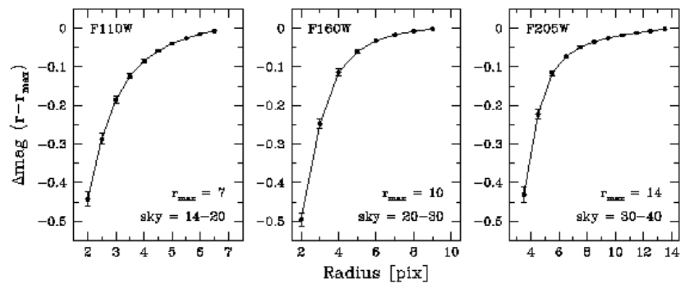
  Fig. 1.—: Cumulative growth curves for the F110W, F160W and F205W bands derived by DAOGROW. Aperture and inner and outer sky radii are listed in each panel and in Table 2. One pixel equals $0\farcs 075$.

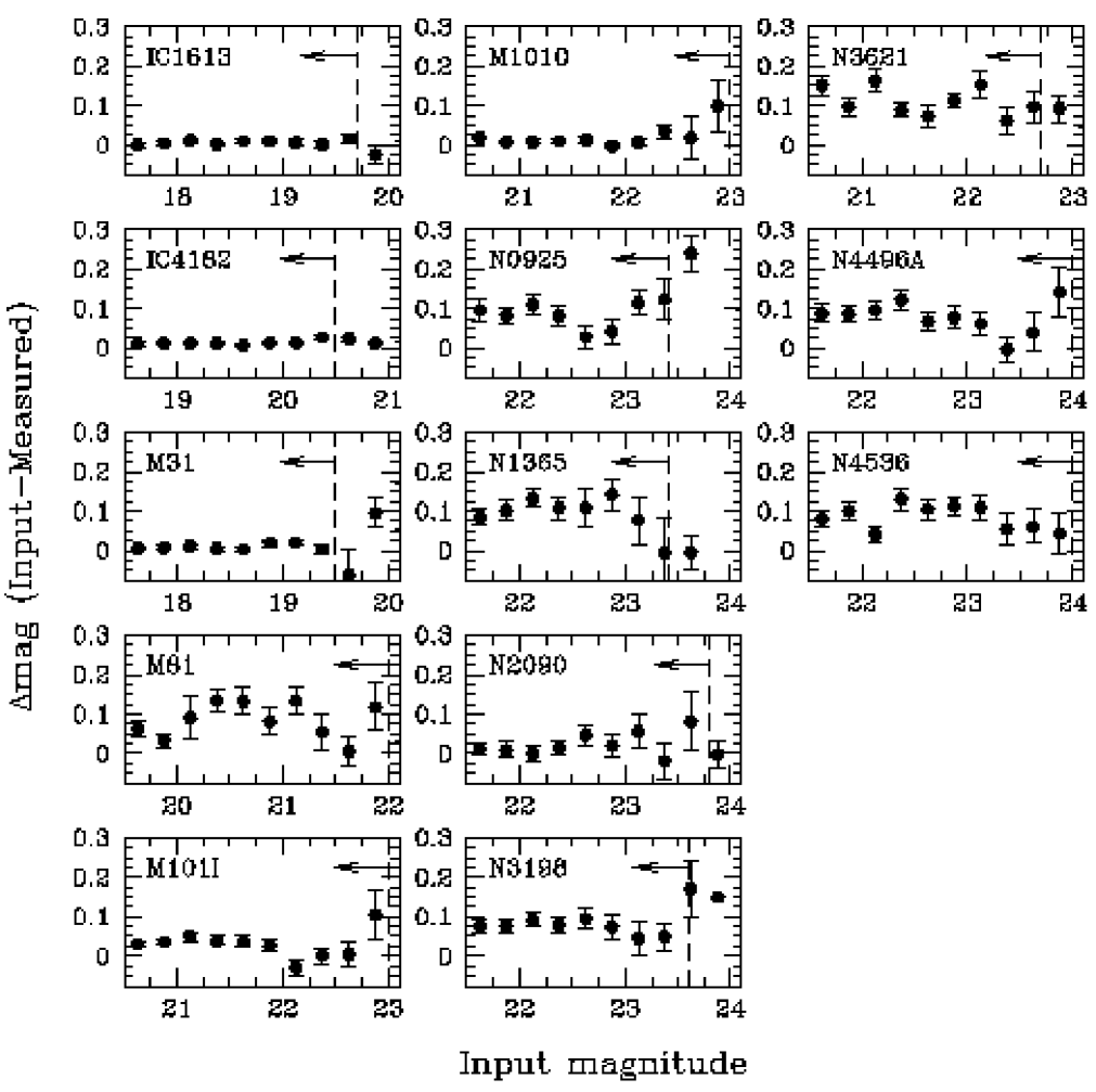
  Fig. 2.—: (a) Results of the photometric recovery tests described in §3.3. Each panel represents one of the field/filter combinations which yielded useful data. Input magnitudes are plotted on the ordinate, while the abscissa shows differences between the input and the recovered magnitudes. Averages over 0.25 mag are plotted using filled circles. The dashed vertical lines mark the faint end of the Cepheid distribution.

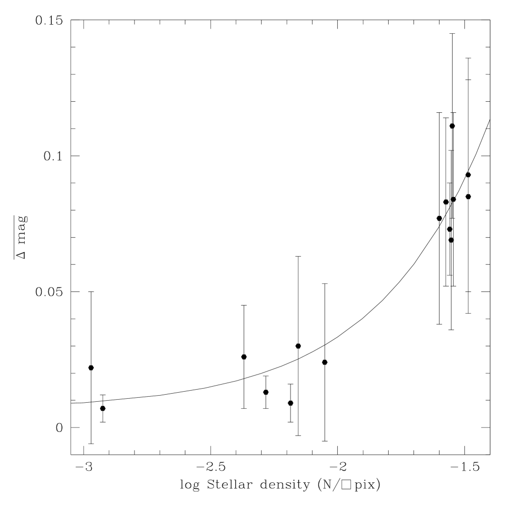
  Fig. 2.—: (b) Results of the photometric recovery tests described in §3.3. Correlation between stellar density and crowding bias; filled circles represent the data found in Table 3. The solid line is derived from a linear least-squares fit to the data.

  Fig. 3.—: Comparison of ground-based and HST $H$-band photometry for bright, isolated stars in the IC 1613 field listed in Table 4. A mean offset of $0.011\pm 0.061$ mag is indicated by solid and dashed lines.

  Fig. 4.—: Histogram of radial distances between predicted positions of our variables and the location of the nearest object in the frame. We rejected 11 candidates whose distance between these two positions was larger than 1.5 pixels.

  Fig. 5.—: (a) Color-color diagram for the 82 candidates which passed the astrometry test. Filled and open symbols indicate the candidates that passed and failed this test, respectively. The solid line is a least-squares fit to a color/color relation with a slope of 1.72 (see text for details).

  Fig. 5.—: (b) Histogram of the deviations from the best-fit line of Fig 5a. We rejected 12 candidates with deviations larger than twice the rms.

  Fig. 6.—: (a) Finding charts for all fields used in this work. The images are full-frame F160W mosaics, spanning $\sim 24\arcsec$. The galaxy name and the STScI-assigned mosaic identification are displayed in each image. Small circles indicate the location of the Cepheids used in this work. The variable names match those of Table 5.

  Fig. 6.—: (b) (continued)

  Fig. 6.—: (c) (continued)

  Fig. 6.—: (d) (continued)

  Fig. 6.—: (e) (continued)

  Fig. 6.—: (f) (continued)

  Fig. 7.—: (a) Individual finding charts for all Cepheids used in this work. Each box is 38 pixels or $\sim 3\arcsec$ on a side. Cepheids are marked by a small circle. The designation of each star is shown in the upper-left corner of each box.

  Fig. 7.—: (b) (continued)

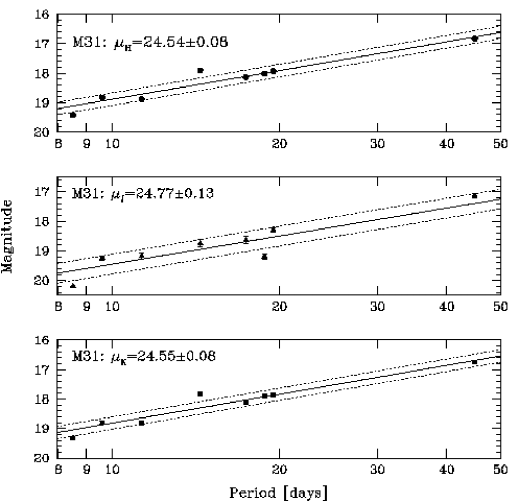
  Fig. 8.—: (a) Near-infrared Period-Luminosity relations for all field/filter combinations. Field name, observed distance modulus and its uncertainty appear in the top-left corner of each panel. Solid lines indicate fitting results while dashed ones indicate the rms uncertainties.

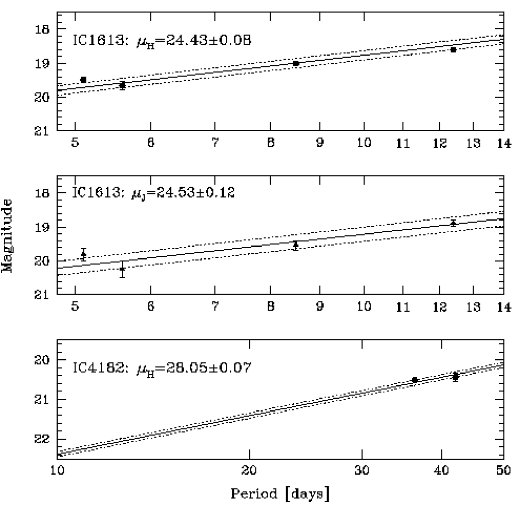
  Fig. 8.—: (b) (continued)

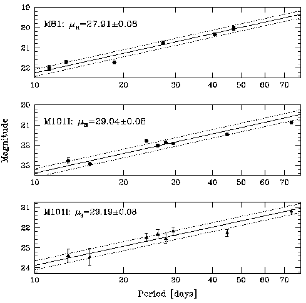
  Fig. 8.—: (c) (continued)

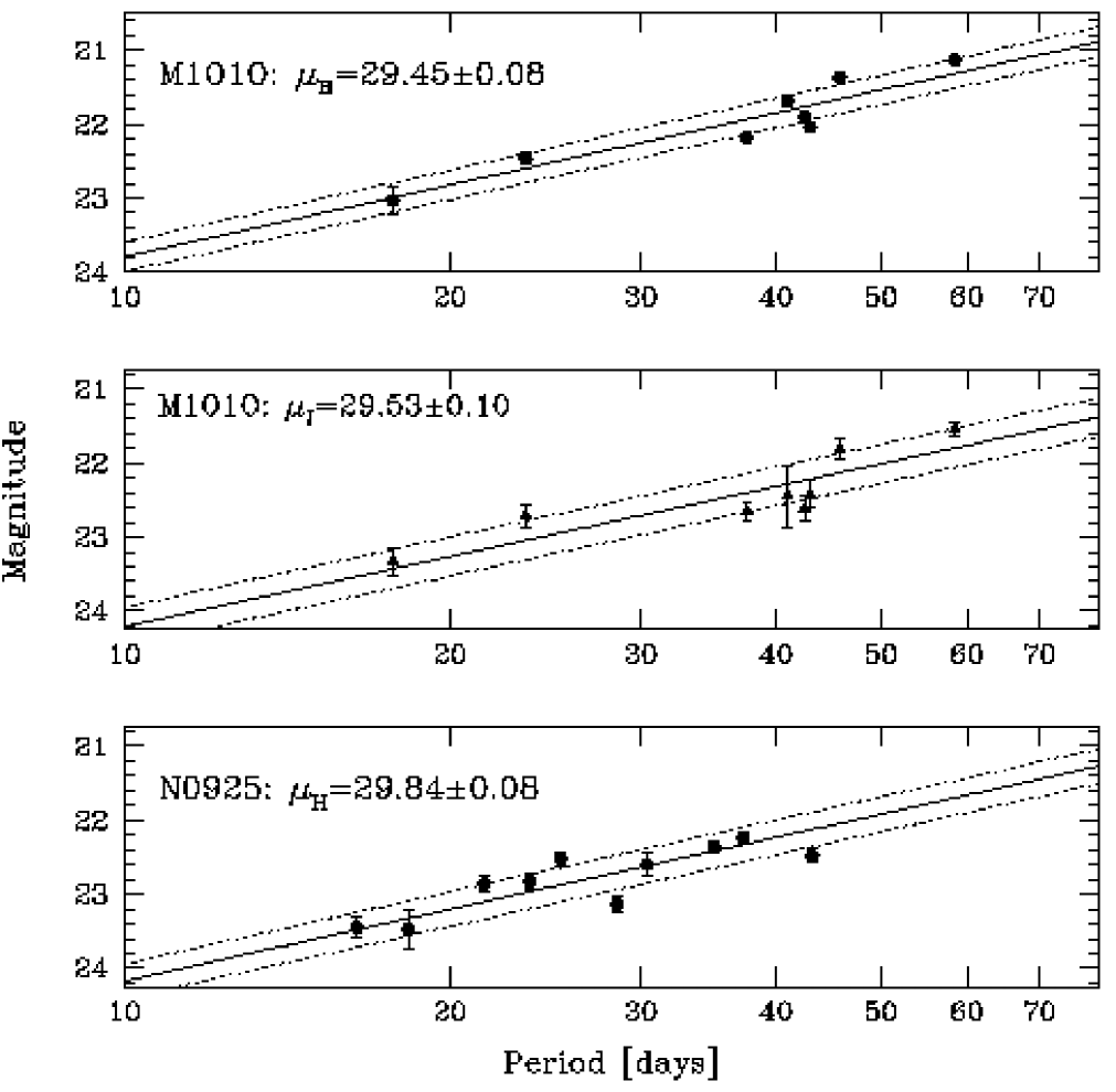
  Fig. 8.—: (d) (continued)

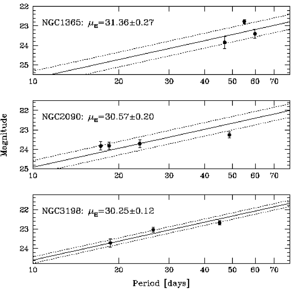
  Fig. 8.—: (e) (continued)

  Fig. 8.—: (f) (continued)

  Fig. 9.—: (a) $V$ and $I$-band Period-Luminosity relations for the fields used in this work. Notation is identical to Figures 8a-f.

  Fig. 9.—: (b) (continued)

  Fig. 9.—: (c) (continued)

  Fig. 9.—: (d) (continued)

  Fig. 9.—: (e) (continued)

  Fig. 10.—: Simulated M101 Inner fields, based on our observations of M31 (right) and M81 (left) fields. These were used to study the effects of blending in our M101 Inner Cepheids.

  Fig. 11.—: Period-Luminosity relations of our simulated M101 Inner fields shown in Figure 10. Filled triangles indicate the input magnitudes of the Cepheids (as observed in our original M31 and M81 fields). Circles represent the recovered magnitudes for the same variables. Filled and open circles are used to indicate whether the recovered Cepheids would have passed or failed the color-color test of §3.1. Dashed and solid lines denote the P-L fits of the input and recovered magnitudes, respectively.

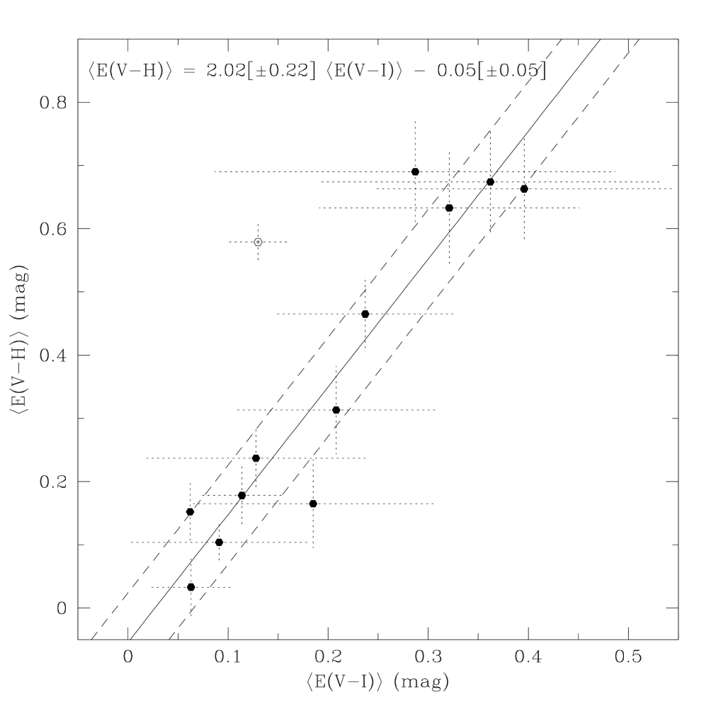
  Fig. 12.—: A test of the correlation between $\langle E(V\!-H)\rangle$ and $\langle E(V\!-I)\rangle$ for our fields. Filled circles represent the crowding-corrected color excesses for our fields. The open circle corresponds to NGC 3198, which was rejected from the fit. The solid line is a least-squares fit to the data, while the dashed lines indicate the rms uncertainty of the fit.

References

- Baade & Swope (1965) Baade, W. & Swope, H.H. 1965, AJ, 70, 212
- Cardelli et al. (1989) Cardelli, J.A., Clayton, G.C. & Mathis, J.S. 1989, ApJ, 345, 245
- Freedman (1988) Freedman, W.L. 1988, ApJ, 326, 691
- Freedman & Madore (1990) Freedman, W.L. & Madore, B.F. 1990, ApJ, 365, 186
- Freedman et al. (1994) Freedman, W.L. et al. 1994, ApJ, 427, 628
- Freedman et al. (2001a) Freedman, W.L., et al. 2001, ApJ, in press
- Freedman et al. (2001b) Freedman, W.L., et al. 2001, in preparation
- Gibson et al. (2000) Gibson, B.K., et al. 2000, ApJ, 529, 723
- Kelson et al. (1996) Kelson, D.D., et al. 1996, ApJ, 463, 26
- Kelson et al. (1999) Kelson, D.D., et al. 1999, ApJ, 514, 614
- Kennicutt et al. (1998) Kennicutt, R.C., et al. 1998, ApJ, 498, 181
- Kochanek (1997) Kochanek, C.S. 1997, ApJ, 491, 13
- Mochejska et al. (2000) Mochejska, B.J., Macri, L.M., Sasselov, D.D. & Stanek, K.Z. 2000, AJ, 120, 810
- Mochejska et al. (2001) Mochejska, B.J., Macri, L.M., Sasselov, D.D. & Stanek, K.Z. 2001, in preparation
- Mould et al. (2000) Mould, J.R., et al. 2000, ApJ, 529, 786
- Persson et al. (1992) Persson, S.E., et al. 1992, PASP, 104, 204
- Persson et al. (1998) Persson, S.E., et al. 1998, AJ, 116, 2475
- Persson et al. (2001) Persson, S.E., et al. 2001, in preparation
- Phelps et al. (1998) Phelps, R.L., et al. 1998, ApJ, 500, 763
- Rawson et al. (1997) Rawson, D.M., et al. 1997, ApJ, 490, 517
- Saha et al. (1994) Saha, A., et al. 1994, ApJ, 425, 14
- Saha et al. (1996) Saha, A., et al. 1996, ApJ, 466, 55
- Saha et al. (1999) Saha, A., et al. 1999, ApJ, 522, 802
- Silbermann et al. (1996) Silbermann, N.A., et al. 1996, ApJ, 470, 1
- Silbermann et al. (1999) Silbermann, N.A., et al. 1999, ApJ, 515, 1
- Stetson (1990) Stetson, P.B. 1990, PASP, 102, 932
- Stetson (1994) Stetson, P.B. 1994, PASP, 106, 250
- Stetson (1998) Stetson, P.B. 1998, PASP, 110, 1448
- Stetson et al. (1998) Stetson, P.B., et al. 1998, ApJ, 508, 491
- Thompson (1993) Thompson, R.I. 1993, Advances in Space Research,vol. 13, no. 12, p. 509
- Udalski et al. (1999) Udalski, A., et al. 1999, Ac.A., 49, 223