The far-infrared–submm spectral energy distribution of high-redshift quasars

Abstract

We combine photometric observations of high-redshift ($z>4$) quasars, obtained at submillimetre (submm) to millimetre wavelengths, to obtain a mean far-infrared (FIR) (rest-frame) spectral energy distribution (SED) of the thermal emission from dust, parameterised by a single temperature ($T$) and power-law emissivity index ($\beta$). Best-fit values are $T=41\pm 5{\rm\thinspace K}$, $\beta=1.95\pm 0.3$. Our method exploits the redshift spread of this set of quasars, which allows us to sample the SED at a larger number of rest wavelengths than is possible for a single object: the wavelength range extends down to $\sim 60$ $\mu$m, and therefore samples the turnover in the greybody curve for these temperatures. This parameterisation is of use to any studies that extrapolate from a flux at a single wavelength, for example to infer dust masses and FIR luminosities.

We interpret the cool, submm component as arising from dust heated by star-formation in the quasar’s host galaxy, although we do not exclude the presence of dust heated directly by the AGN. Applying the mean SED to the data, we derive consistent star-formation rates $\sim$1000$\hbox{$\rm\thinspace M_{\odot}$}{\rm\thinspace yr}^{-1}\,$and dust masses $\sim 10^{9}\hbox{$\rm\thinspace M_{\odot}$}$, and investigate a simple scheme of AGN and host-galaxy coevolution to account for these quantities. The timescale for formation of the host galaxy is 0.5–1Gyr, and the luminous quasar phase occurs towards the end of this period, just before the reservoir of cold gas is depleted. Given the youth of the Universe at $z=4$ (1.6Gyr), the coexistence of a massive black hole and a luminous starburst at high redshifts is a powerful constraint on models of quasar host-galaxy formation.

1 INTRODUCTION

Cosmological studies at FIR–submm wavelengths are an essential complement to optical investigations, in that the dust that extinguishes the optical/UV light from AGN or massive stars is that which thereby shines in the infrared. This effect should not be underestimated: the integrated energy density in each of the FIR and optical extragalactic background light is comparable (Puget et al. 1996; Hauser et al. 1998). It has been suggested that cosmological submm sources are high-redshift equivalents of ULIRGs, their luminosity deriving from bursts of dust-obscured star-formation accompanying the assembly of massive elliptical galaxies, in the course either of gas-rich hierarchical major-mergers or ab initio monolithic collapse (Barger, Cowie & Sanders, 1999, and references therein). However, such speculations are difficult to confirm via direct optical follow-up, because of the large beam-sizes of current submm telescopes, and because the dust obscuration necessarily makes the sources optically faint.

An alternative approach is to study the submm properties of well-characterised classes of objects, whose precisely-known positions and redshifts, physical properties and population statistics, facilitate follow-up observations and interpretation. To this end, we have been studying dust continuum and CO emission from luminous ($M_{B}\la-27.5$), high-redshift ($z\ga 4$) quasars. At low redshifts, the hosts of luminous quasars are invariably massive elliptical galaxies (Bahcall et al. , 1997; McLure et al. , 1999). In the local Universe, massive black holes, fossil remnants of AGN now starved of fuel, are found in the cores of most galactic bulges; moreover, their mass is correlated with the stellar mass of the surrounding spheroid, $M_{\rm bh}=6\times 10^{-3}M_{\rm sph}$ (Magorrian et al. , 1998). This correlation hints at a deep connection between black-hole build-up through accretion and star-formation in the host galaxy. Attributing the submm-luminosity of high-redshift quasars to star-formation therefore accords with the speculations about the origins of the submm sources.

Before one can estimate physical quantities, such as dust temperature and star-formation rate, it is necessary to characterise the form of the dust-emission spectrum of these objects. It is also important to quantify variations of the SED with object class, luminosity or redshift, otherwise, if one adopts a single template for all sources, it is not legitimate to adopt more than one derived parameter as an indicator of physical status. In fitting thermal SEDs, however, we are constrained by the paucity of photometric data, and often it is inappropriate to fit both the emissivity and the temperature as free parameters, when we have only three or four photometric points per source. Previous work, which considered object-by-object temperature fits, adopted an assumed value for the emissivity index (Buffey et al. , in prep.). In contrast, the purposes of this Letter are, first, to investigate the possibility of co-adding data from a sample of luminous, $z\ga 4$ quasars, to find a self-consistent, overall best-fit temperature and emissivity; and to characterise the uncertainties involved in doing so, whether they are due to experimental errors or to physical differences. Finally, we discuss applications of the mean SED, and try to justify the inferred parameters in terms of a simple evolutionary model.

Throughout, we assume a $\Lambda$-dominated cosmology $\Omega_{M}$=0.3, $\Omega_{\Lambda}$=0.7, $H_{0}$=65${\rm\thinspace km}{\rm\thinspace s}^{-1}\,$ Mpc^-1.

2 MEAN ISOTHERMAL SPECTRUM

2.1 Data

The $z>4$ datasets are from our work with IRAM (1.25 mm) and JCMT (SCUBA 850 $\mu$m, 750 $\mu$m, 450 $\mu$m and 350 $\mu$m; UKT14 800 $\mu$m) as described in companion papers (Isaak et al. 1994; Omont et al. , 1996a; Buffey et al. , in prep.); and 350 $\mu$m CSO photometry is from Benford et al. (1999). Additionally, we include the $z=3.91$ quasar APM08279$+$5255 (Lewis et al. 1998). All the sources have been detected at least four different wavelengths. An important caveat is that the quoted statistical uncertainties do not reflect the systematic errors due to flux calibration. Therefore, we assume calibration errors, combined in quadrature with the random uncertainties, of 20 percent.

Table 1: Summary of SED parameters used by other authors

Authors	Sample	$\frac{\overline{L_{\rm fir}}}{\hbox{$\rm\thinspace L_{\odot}$}}$	$\overline{T}$	$\overline{\beta}$
Dunne et al.	SLUGS	1011	36	1.3
Carico et al.	LIRGs	1011.5	32	1.6
Lisenfeld et al.	LIRGs	1011.5	38	1.6
Benford et al.	High-$z$ objects	1013	52	1.5†
Hughes et al.	High-$z$ objects	1013	50†	1.5†
McMahon et al.	$z>4$ quasars	1013	50†	1.5†
This work	$z>4$ quasars	1013	42	1.9

^† values presumed, not determined

2.2 Assumptions

The rest-frame far-infrared (FIR) SED can be described by a modified blackbody spectrum, assuming that the grains are in equilibrium with the radiation field and that the dust cloud is optically-thin at submm wavelengths: $S_{\nu}\propto\frac{\nu^{3+\beta}}{e^{\frac{h\nu}{kT}}-1}.$ Note, however, that some ultraluminous starbursts (such as Arp220; Rowan-Robinson & Efstathiou, 1993) are optically thick at the shortest rest-wavelengths sampled by the present data (60$\mu$m). This method determines the most effective isothermal parameterisation of the long-wavelength emission, a simple, convenient description that is frequently adopted (e.g. Benford et al., 1999; Lisenfeld, Isaak & Hills, 2000; Dunne et al., 2000), though in reality, a distribution of dust temperatures is likely. Shorter wavelength radiation, in the near-to-mid infrared region ($\sim$10 $\mu$m rest-frame), is likely to be contaminated by the hotter dust that absorbs the harder continuum due to the AGN itself (e.g. Rowan-Robinson, 1995). The contribution from star formation, on the other hand, emerges in the submillimetre region. To assess the contamination of the submillimetre luminosity due to the AGN component requires better mid-infrared constraints than exist for all but a few high-redshift quasars (see, for example, Rowan-Robinson, 2000). We therefore simply assume that the component extracted by our fitting procedure is appropriate for the extrapolation of a far-infared luminosity ($L_{\rm FIR}$) from which a star formation rate is to be calculated. We caution, however, that the unforeseen presence of a hot component could skew the fit to higher temperatures, leading us to overestimate the star formation rate.

2.3 Method

Adopting $T$ and $\beta$ as free parameters, we employ a $\chi^{2}$-minimisation procedure to determine the best single-component fit to the data, which is coadded in a self-consistent way. A subtlety arises because for a given observed wavelength, the range of objects’ redshifts causes us to sample their spectra at different rest wavelengths. Therefore, if we choose to normalise the data at a given rest wavelength, a spectrum must be assumed so that an extrapolation to this reference from the nearest observed data point can be performed. The best-fit spectrum thus determined then itself becomes the template for the extrapolation, and the process is iterated. In practice, this procedure converges to a solution rapidly (i.e. without roaming around parameter space) so for these datasets at least, we conclude that the overall $\chi^{2}$-minimised fit is, indeed, the best self-consistent solution.

Figure 1: Contours of $\chi^{2}$, in $\beta-T$ space, for our combined photometry of $z>4$ quasars. The star-shaped symbol indicates the best-fit position, and both 1– and 2–$\sigma$ contours are plotted (solid). For comparison, the best-fit and 1– and 2–$\sigma$ contours for local LIRGs (from Lisenfeld, Isaak & Hills, 1999) (asterisk and dashed), and for local galaxies (from Dunne et al. , 2000) (cross and dotted), are also shown. The dot–dashed line is a locus of constant luminosity derived from the best-fit $T$ and $\beta$, for constant 850 $\mu$m flux at $z=4.5$.

Figure 2: The best-fit, rest-frame SED, with renormalised data points. Each separate symbol denotes a different quasar: BR1202$-$0725 (filled circles), APM08279$+$5255 (open circles), BRI1335$-$0417 (squares), BR1117$-$1329 (stars), BRI0952$-$0115 (upright triangles), BR1033$-$0327 (inverted triangles), BR1144$-$0723 (diamonds). The solid line corresponds to $T=41{\rm\thinspace K}$, $\beta=1.95$, the $\chi^{2}$-minimised best fit to these points, while the dashed and dotted lines represent the best fits to the data of Lisenfeld et al. and Dunne et al. (as in Figure 2). The dot–dashed line is the starburst model of Rowan-Robinson & Efstathiou (1993). The curves are normalised at 850 $\mu$m/(1+4.5).

Figure 3: Ratio of observed flux at 850 $\mu$m to that at 1250 $\mu$m— i.e. , the conversion between typical observations made with JCMT/SCUBA and with IRAM respectively. The solid lines are best fit (centre) and $\pm$1– and 2–$\sigma$ . The apparent convergence at $z\sim 6$ is due to the tight bunch of data points near rest-frame 150 $\mu$m (see Figure 2). The dashed and dotted lines correspond, as in Figures 1 and 2, to the best-fits for the Lisenfeld et al. and Dunne et al. samples, whilst the dot–dashed line depicts Arp220.

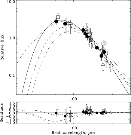
2.4 Results

The $\chi^{2}$ contours are shown in Figure 1, while the renormalised data and best-fit SED are plotted in Figure 2. The best self-consistent fit corresponds to $\beta=1.95\pm 0.3$, $T=41\pm 5{\rm\thinspace K}$ (1$\sigma$ errors). A similar procedure applied to the low-redshift, less-lumimous samples of LIRGs (Lisenfeld, Isaak & Hills, 1999) and local galaxies (Dunne et al. , 2000) gives results inconsistent at the $>2\sigma$ level (Figure 1).

We can use the $\chi^{2}$ contours to predict the outcome of curve-fitting in which $\beta$ is held fixed, while the temperature is varied. For other studies of high-redshift quasar SEDs, the $\beta=1.5$ adopted by Benford et al. (1999) and Buffey et al. (in prep.) would give $T$=50 K as mean best-fit, which is indeed close to that found by those authors, and consistent with the $T$=50 K assumed by McMahon et al. (1999). Variation in luminosities (hence, eventually, star-formation rates) estimated from such best-fits do not vary substantially, because $L_{\rm FIR}\propto(3+\beta)!\times T^{4+\beta}$, whilst the best-fit $T$ is monotonically decreasing with $\beta$: the dot–dashed line in Figure 1, a locus of constant luminosity, illustrates this. This is to be expected, since luminosity is an integral under the curve defined by the data points. On the other hand, using best fits to the datasets consisting of other objects (listed in Table 1), would give a discrepancy in luminosity of up to a factor three at the redshifts of our quasars.

3 APPLICATIONS

In this section, we discuss some applications for observation, and implications for interpretation, of this mean SED.

3.1 Millimetre–submillimetre spectral index

The steep slope of cool, thermal SEDs over the mm–submm range makes knowledge of the precise spectral shape important, when comparing data obtained with different instruments operating at different wavelengths. Consider, for example, the spectral index between 850 $\mu$m and 1.25mm, appropriate for converting between JCMT/SCUBA and IRAM data, respectively. The ratio of fluxes as a function of redshift for our best fit to $z>4$ quasars, together with the fits to LIRGs and local galaxies, is shown in Figure 3. For ease of reference, a linear approximation to the ratio for our best fit, good out to $z\sim 7$, is $R(\frac{850}{1250})\approx 3.7-z/4$.

Table 2: $z>4$ sources used in the fit, from Omont et al. (1996), with measured and extrapolated properties based upon the 850 $\mu$m fluxes of Buffey et al. (in prep.)

Object	$z$	$M_{B}$	$M_{\rm bh}$	$L_{\rm FIR}$	$M_{\rm d}$	$M_{\rm H_{2}}$	$M_{\rm sph}$	$SFR$	$\tau_{\rm sph}$	$z_{\rm max}$	$z_{\rm min}$
			$10^{9}\hbox{$\rm\thinspace M_{\odot}$}$	$10^{13}\hbox{$\rm\thinspace L_{\odot}$}$	$10^{9}\hbox{$\rm\thinspace M_{\odot}$}$	$10^{11}\hbox{$\rm\thinspace M_{\odot}$}$	$10^{11}\hbox{$\rm\thinspace M_{\odot}$}$	$10^{3}\frac{\hbox{$\rm\thinspace M_{\odot}$}}{\rm yr}$	$10^{9}{\rm\thinspace yr}$
BRI0952$-$0115	4.43	$-$28.0	5.5	2.0	1.7	1.4	9.1	1.2	0.9	9.5	2.9
BR1202$-$0725	4.69	$-$28.8	11	5.8	5.0	4.1	19	3.5	0.7	7.9	3.3
BR1335$-$0417	4.40	$-$27.6	3.8	2.0	1.7	4.3	6.3	1.2	0.6	6.9	3.2
BR1033$-$0327	4.50	$-$27.9	5.0	1.0	0.8	$<$0.9†	8.3	0.6	1.7	$\infty$	2.3
BR1117$-$1329	3.96	$-$28.2	6.6	1.9	1.7	$<$1.2†	11	1.1	1.2	10	2.5
BR1144$-$0723	4.14	$-$27.7	4.1	1.0	0.9	$<$1.3†	6.9	0.6	1.4	20	2.4
Median Quasar‡	4.5	$-$28.0	5	2	2	1.5	8	1.2	0.7	7.4	3.2

Note: All derivations assume $\Omega_{M}=0.3$, $\Omega_{\Lambda}=0.7$, $H_{0}=65\hbox{${\rm\thinspace km}{\rm\thinspace s}^{-1}\,$}{\rm\thinspace Mpc}^{-1}$

^† 3$\sigma$ upper limits

^‡ represents median of the observed quasars, consistent with an object having $S_{850}\approx 15$mJy and $M_{B}=-28.0$.

3.2 Physical characteristics

Table 2 lists physical properties inferred for each of the quasars contributing to the fit. Dust masses ($M_{\rm d}$) and far-infrared luminosities ($L_{\rm FIR}$) are calculated as in McMahon et al. (1999), though with our new $T$ and $\beta$. The final stellar mass of the host spheroid ($M_{\rm sph}$) is estimated using the local relation between bulge and black hole mass (Magorrian et al. , 1998), with the latter calculated from the absolute $B$-band magnitude ($M_{B}$) via simple assumptions about accretion (Section 3.3), and a bolometric correction of 12 after Elvis et al. (1994). Molecular gas masses ($M_{\rm H_{2}}$) are calculated from observed CO emission-line luminosities (Omont et al. 1996b; Guilloteau et al. 1997, 1998), using a conversion factor $M_{\rm H_{2}}/L^{\prime}_{\rm CO}=4.5\hbox{$\rm\thinspace M_{\odot}$}({\rm\thinspace K}\hbox{${\rm\thinspace km}{\rm\thinspace s}^{-1}\,$}{\rm\thinspace pc}^{2})^{-1}$ (Solomon, Downes & Radford, 1992); though we caution that a calibration as much as five times smaller than this has been reported to be more appropriate for some ULIRGs (Downes & Solomon, 1998).

The substantial star-formation rates and far-infrared luminosities might cause us some concern: $L_{\rm fir}\sim L_{B}$, so we should consider whether the AGN itself is an important contributor to the cool dust luminosity. Of course, the equally-substantial quantities of of cool molecular gas ($M_{H_{2}}>10^{11}\hbox{$\rm\thinspace M_{\odot}$}$) make ideal nests for hatching young stars; and stars are required to manufacture the large mass of dust that is observed ($M_{\rm d}>10^{9}\hbox{$\rm\thinspace M_{\odot}$}$). Moreover, the CO(5–4)/1.35mm-continuum of BR1202$-$0725 has been resolved into two components (Omont et al. , 1996), only one of which coincides with the quasar, the other showing no sign of AGN activity. Yun et al. (2000) have detected the three CO-luminous quasars at 1.4  GHz: the reported fluxes are consistent with synchrotron emission from supernova remnants, and imply star-formation rates $\sim$1000$\hbox{$\rm\thinspace M_{\odot}$}{\rm\thinspace yr}^{-1}\,$, in agreement with the submm predictions (Section 3.3, and Table 2). Therefore, although we do not exclude the possibility that some of the submm flux is due to AGN-heating, here we shall explore the hypothesis that it derives wholly from star-formation.

This leaves us with somewhat extraordinary objects, which are not only undergoing intense bursts of dust-obscured star formation, but simultaneously hosting powerful quasars. The age of the Universe at $z=4$ is 1.6 Gyr: this lack of time imposes severe constraints upon the processes governing both central black-hole growth (Turner 1993) and the chemical evolution necessary to supply the large observed dust masses (Edmunds & Eales 1998). The statistics are, currently, very poor (only three $z>4$ objects with CO-detections, biased towards the most luminous objects), nevertheless we assume that the Median Quasar of Table 2 epitomises its class, to guide our quest for a consistent hypothesis.

3.3 Quasar and host galaxy coevolution

The far-infrared luminosity ($L_{\rm FIR}$) can be used to estimate the current star-formation rate, given a stellar Initial Mass Function (IMF) and a prior star-formation history: $SFR/\hbox{$\hbox{$\rm\thinspace M_{\odot}$}{\rm\thinspace yr}^{-1}\,$}=\Psi L_{\rm FIR}/10^{10}\hbox{$\rm\thinspace L_{\odot}$}$. To estimate $\Psi$, we use the stellar population synthesis model of Leitherer et al. (1999), STARBURST99, assuming a constant star-formation rate and that $L_{\rm FIR}=L_{\rm bol}$. A significant cause of uncertainty is due to the choice of IMF: introducing faint, low-mass stars has the effect of increasing the total mass while hardly affecting the luminosity, therefore one must infer a higher star-formation rate for a given $L_{\rm bol}$. We adopt a Salpeter IMF ($\phi(m)\propto m^{-2.35}$, Salpeter 1955) within the mass range $1\hbox{$\rm\thinspace M_{\odot}$}<m<100\hbox{$\rm\thinspace M_{\odot}$}$. $\Psi$ depends much more weakly upon metallicity, and upon the age of the burst for lifetimes longer than $\sim 10^{7}{\rm\thinspace yr}$. We take $\Psi=0.6$, which corresponds to a metallicity $Z=Z_{\odot}$ and an age $t\approx 0.5{\rm\thinspace Gyr}$. Another source of uncertainty is the fraction of starlight that is intercepted by dust; here we make the simplifying assumption that this fraction is unity. Star-formation rates thus derived are presented in Table 2.

The spheroid-formation timescales in Table 2 correspond to the total time required to convert the inferred spheroid masses from gas into stars, at constant star-formation rate; not forgetting gaseous material expelled, from massive stars, as winds and supernovae (we assume a return fraction of $\approx$20 percent). It is through this outflow process that the interstellar medium (ISM) becomes chemically enriched: if half the mass in metals condenses into dust, then chemical yields derived from stellar evolution models (e.g. Maeder, 1992) predict that $\sim$1 percent of the mass processed through stars (for our IMF) is returned to the ISM in the form of dust— neglecting however the intricacies of dust-destruction and -dispersion by supernovae. Thus, after 0.5 Gyr, the stellar mass of the Median Quasar would be $\approx$6$\times 10^{11}\hbox{$\rm\thinspace M_{\odot}$}$, its gas mass is $\approx$2$\times 10^{11}\hbox{$\rm\thinspace M_{\odot}$}$, and its dust mass is $\approx$3$\times 10^{9}\hbox{$\rm\thinspace M_{\odot}$}$— near the maximum it can attain for these parameters, before becoming recycled into long-lived stellar remnants (Edmunds & Eales, 1998).

Meanwhile, to describe the evolution of the AGN, we adopt the simplest assumptions about accretion onto a massive black hole (Rees, 1984): that the mass flow $\dot{M}_{\rm acc}$ is regulated by radiation pressure— i.e. accretion occurs at the Eddington rate— and that the accretion efficiency $\epsilon\sim 0.1$, so

$$L_{\rm bol}=\epsilon\dot{M}_{\rm acc}c^{2}=\frac{4\pi Gm_{\rm p}cM_{\rm bh}}{\sigma_{\rm T}}=3\times 10^{13}\frac{M_{\rm bh}}{10^{9}\hbox{$\rm\thinspace M_{\odot}$}}\hbox{$\rm\thinspace L_{\odot}$},$$ (1)

where $\sigma_{\rm T}=6.65\times 10^{-25}{\rm\thinspace cm}^{2}$ is the Thomson cross-section, and $m_{\rm p}=1.67\times 10^{-24}{\rm\thinspace g}$ is the proton mass. The accretion rate is $\dot{M}_{\rm acc}=\frac{22}{\epsilon/0.1}\frac{M_{\rm bh}}{10^{9}\hbox{$\rm\thinspace M_{\odot}$}}\hbox{$\hbox{$\rm\thinspace M_{\odot}$}{\rm\thinspace yr}^{-1}\,$}$ and the mass $e$-folding time for the growth of the black hole is $\tau_{\rm bh}=\frac{\epsilon M_{\rm bh}c^{2}}{L_{\rm bol}}=\frac{\epsilon}{0.1}\times 4.5\times 10^{7}$ yr. Supposing that Eddington-limited accretion starts to apply above a seed black hole mass of about $10^{6}\hbox{$\rm\thinspace M_{\odot}$}$ (Haehnelt, Natarajan & Rees, 1998), it would take $\sim$0.5 Gyr to build the required quasars— close to the star-forming lifetime of the host galaxy, discussed above.

The total (baryonic) mass of the galaxy has been inferred from the black hole mass by taking the local remnant black hole–bulge correlation (Magorrian et al. . 1998). Critics may object that we do not measure the final mass of the black hole, because we observe it while it is still actively accreting. However, by the time the black hole’s mass is $5\times 10^{9}\hbox{$\rm\thinspace M_{\odot}$}$, its Eddington accretion rate is 100$\hbox{$\rm\thinspace M_{\odot}$}{\rm\thinspace yr}^{-1}\,$and rising, and it is competing with star-formation ($\sim$1000$\hbox{$\rm\thinspace M_{\odot}$}{\rm\thinspace yr}^{-1}\,$) for the rapidly-diminishing supply of cold gas. In the absence of inflow, this cannot be sustained for long. Therefore, we obtain one consistent scheme by assuming that the black holes’ masses do not grow much greater than the values deduced from the quasar light. This is in accord with the measurements of remnant black hole masses in the local Universe, which give at most $10^{9.5}\hbox{$\rm\thinspace M_{\odot}$}$.

The quantities $z_{\rm max}$ and $z_{\rm min}$ in Table 2 bracket the redshift range over which the quasars are forming stars, based upon the inferred spheroid mass and constant star-formation rate. The severity of the time constraint at high redshifts is dramatically illustrated, especially for BR1033$-$0327, which has a star-forming lifetime longer than the age of the Universe at its redshift. In this case, we could resolve the dilemma by invoking a different IMF and star-formation/accretion histories: for example, exponential gas-consumption and a phase of super-Eddington accretion, or more low-mass stars leading to a higher star-formation rate, would give rather shorter lifetimes. We refrain from investigating this here, however, for lack of space and data-volume, but we shall examine the problem in later papers.

4 CONCLUSIONS

We have constructed a mean SED, over the rest-frame wavelength range 60–300 $\mu$m, for luminous $z>4$ quasars, assuming an isothermal dust spectrum. We consider applications of this SED, such as the conversion between commonly-used submm/mm wavebands, and the estimation of star-formation rates and dust masses. Using the observed local remnant black hole to bulge mass relation to estimate the initial gas mass, we deduce star-formation timescales and sketch a simple evolutionary scenario.

Estimation of star-formation rate and dust and gas masses obtained through submm–mm observations are potentially important constraints on models of quasar–host-galaxy coevolution. However, the correct interpretation of such information requires detailed knowledge of the SED and its variation with parameters such as redshift and luminosity. Otherwise, it is misleading to treat, as independent, quantities whose derivation follows from a single data point. Although we have here determined a “mean” SED, we do not suggest that all high-redshift quasars possess a unique dust temperature: much of the scatter about the mean is very likely real. The data are not yet extensive enough to justify a more detailed treatment, particularly since only the most luminous objects are suitable for multi-wavelength photometry.

We emphasise, too, that it is important to justify the large derived star-formation rates and dust masses in terms of the evolution of stellar populations and chemical abundances: the simple treatments frequently adopted are not necessarily misleading, but neither are they immune to justified criticism. Employing a skeletal evolutionary scheme, a consistent account emerges, within the many uncertainties, if we identify submm-luminous, high-redshift quasars with an early, gas-rich phase in the formation of massive galaxies, at about the time when the dust mass reaches its maximum, after the AGN has grown sufficiently luminous for it to be identified as a bright quasar and just before star-formation has depleted the fuel-supply upon which it subsists. We estimate that this quasar–starburst phase is short, lasting for little longer than 0.5 Gyr, though by changing our assumptions— for example, regarding the IMF or early accretion and star-formation history—, further consistent models could be constructed. Forthcoming observational results (Isaak et al. , in prep.) will improve statistics and permit refinement of these speculations.

References

- [Bahcall et al. 1997] Bahcall J.N., Kirhakos S., Saxe D.H., Schneider D.P., 1997, ApJ, 479, 642
- [Barger, Cowie & Sanders 1999] Barger A.J., Cowie L.L., Sanders D.B., 1999, ApJ, 518, L5
- [Downes & Solomon 1998] Downes D. & Solomon P.M., 1998, ApJ, 507, 615
- [Dunne et al. 2000] Dunne L., Eales S., Edmunds M., Ivison R., Alexander P., Clements D.L., 2000, MNRAS, 315, 115
- [Edmunds & Eales1998] Edmunds M.G, Eales S.A., 1998, MNRAS 299, L29
- [Elvis et al. 1994] Elvis M. et al., 1994, ApJS, 95, 1
- [Guilloteau et al. 1997] Guilloteau S., Omont A., McMahon R.G., Cox P., Petitjean P., 1997, A&A, 328, L1
- [Guilloteau et al. 1997] Guilloteau S., Omont A., Cox P., McMahon R.G., Petitjean P., 1999, A&A, 349, 363
- [Haehnelt, Natarajan & Rees1998] Haehnelt M.G., Natarajan P., Rees M.J., 1998, MNRAS, 300, 817
- [Hauser et al. 1998] Hauser M.G. et al., 1998, ApJ, 508, 25
- [Hughes, Dunlop & Rawlings 1997] Hughes D.H., Dunlop J.S., Rawlings S., 1997, MNRAS, 289, 766
- [Isaak et al. 1994] Isaak K.G., McMahon R.G., Hills R.E., Withington S., 1994, MNRAS, 269, L28
- [Leitherer et al. 1999] Leitherer C. et al. , 1999, ApJS, 123, 3
- [Lewis et al. 1998] Lewis G.F., Chapman S.C., Ibata R.A., Irwin M.J., Totten E.J., 1998, ApJL, 505, 1
- [Lisenfeld, Isaak & Hills 2000] Lisenfeld U., Isaak K.G., Hills R., 2000, MNRAS, 312, 433
- [Maeder1992] Maeder A., 1992, A&A, 264, 105
- [Magorrian et al. 1998] Magorrian J. et al. , 1998, AJ, 115, 2285
- [McLure et al. 1999] McLure R.J., Kukula M.J, Dunlop J.S., Baum S.A., O’Dea C.P., Hughes D.H., 1999, MNRAS, 308, 377
- [McMahon et al. 1994] McMahon R.G., Omont A., Bergeron J., Kreysa E., Haslam C.G.T., 1994, MNRAS, 267, L9
- [McMahon et al. 1999] McMahon R.G., Priddey R.S., Omont A., Snellen I., Withington S., 1999, MNRAS 309, L1
- [Omont et al. 1996a] Omont A., McMahon R.G., Cox P., Kreysa E., Bergeron J., Pajot F., Storrie-Lombardi L.J., 1996a, A&A, 315, 1
- [Omont et al. 1996b] Omont A., Petitjean P., Guilloteau S., McMahon R.G., Solomon P.M., Pécontal, E., 1996b, Nature, 382, 428
- [Puget et al. 1996] Puget J.-L. et al., 1996, A&A, 308, L5
- [Rees1984] Rees M.J., 1984, ARA&A, 22, 471
- [Rowan-Robinson1995] Rowan-Robinson M., 1995, MNRAS, 272, 737
- [Rowan-Robinson2000] Rowan-Robinson M., 2000, MNRAS, 316, 885
- [Rowan-Robinson & Efstathiou1993] Rowan-Robinson M. & Efstathiou A., 1993, MNRAS, 263, 675
- [Salpeter1955] Salpeter E.E., 1955, ApJ, 121, 161
- [Yun et al. 2000] Yun M.S., Carilli C.L., Kawabe R., Tutui Y., Kohno K., Ohta K., 2000, ApJ, 528, 171