Gravitational Memory ?
— a Perturbative Approach —

Abstract

It has been pointed out that the value of the gravitational “constant” in the early universe may be different from that at present. In that case, it was conjectured that primordial black holes may “remember” the value of the gravitational constant in the early universe. The present analysis shows that this is not the case, at least in certain contexts.

Department of Physics, Waseda University,
Shinjuku, Tokyo 169-8555, Japan

Astronomy Unit, Queen Mary and Westfield College,
University of London, London E1 4NS, England

1 Introduction

In the early universe, black holes may have been formed due to inhomogeneous initial conditions, phase transitions, or other mechanisms. They are called primordial black holes (PBHs). The mass of the PBHs is of order the mass contained within the Hubble horizon at the formation epoch. Hawking [1] discovered that black holes emit radiation due to the quantum effects of the curved spacetime. PBHs therefore lose mass and those lighter than $\sim 10^{15}\mbox{g}$ may contribute to the cosmic gamma-ray background and spoil the success of the big bang nucleosysthesis scenario. PBHs heavier than that may dominate the density of the universe at present. Therefore the fraction $\beta$ of the universe which may have gone into PBHs can be constrained from various cosmological observations (Carr [2]).

It has been pointed out that gravity in the early universe may have been dilatonic, since this arises naturally as a low-energy limit of string theory. In such theories, the gravitational “constant” is given by a function of a scalar field which couples non-minimally with gravity. In particular, the gravitational constant in the early universe may have been different from that at the present epoch. The Brans-Dicke theory is the simplest such theory of gravity. Barrow [3] considered PBHs in Brans-Dicke theory and proposed two scenarios. In scenario A, the gravitational constant at the black hole event horizon is always the same as that at the cosmological particle horizon, i.e., $G_{EH}(t)=G_{PH}(t)$. In scenario B, the gravitational constant at the black hole event horizon is constant with time and therefore always the same as that at the formation epoch, i.e., $G_{EH}(t)=G_{EH}(t_{f})=G_{PH}(t_{f})$. Scenario B corresponds to what is called the gravitational memory, while scenario (A) entails no gravitational memory.

Barrow and Carr [4] obtained observational constraints on $\beta$ in both scenarios. They assumed that the energy emission due to the Hawking radiation is determined by the temperature $T_{H}=(8\pi G_{EH}(t)M)^{-1}$, so that the mass loss rate is $\dot{M}\simeq-(G_{EH}(t)M)^{-2}$. The results for the two scenarios can be significantly different. Subsequently, Carr and Goymer [5] argued that the true situation may be intermediate between Scenario A and Scenario B and this allows other possibilities. Therefore, in order to deduce the history of the early universe from the present observations, it is very important to examine which scenario is realized.

Recently, Jacobson [6] has argued that there is no gravitational memory for a Schwarzschild black hole with a time-varying boundary condition which mimics the cosmological evolution of a scalar field. However, this argument applies only if the black hole is much smaller than the particle horizon, so we must consider more general situations. The purpose of this article is to solve the problem self-consistently for a Friedmann-Robertson-Walker (FRW) background.

2 Basic Equations

The field equations in Brans-Dicke theory are given by

$$R_{\mu\nu}-\frac{1}{2}g_{\mu\nu}R=\frac{8\pi}{\phi}T_{\mu\nu}+\frac{\omega}{\phi^{2}}\left(\phi_{,\mu}\phi_{,\nu}-\frac{1}{2}g_{\mu\nu}\phi_{,\alpha}\phi^{,\alpha}\right)+\frac{1}{\phi}\left(\nabla_{\mu}\nabla_{\nu}\phi-g_{\mu\nu}\Box\phi\right),$$ (1)

$$\nabla_{\mu}T^{\mu\nu}=0,$$ (2)

$$\Box\phi=\frac{8\pi}{3+2\omega}T^{\mu}_{\quad\mu},$$ (3)

where the constant $\omega$ is the Brans-Dicke parameter and $\phi$ is the Brans-Dicke scalar field, which is related to the gravitational constant by $G\sim\phi^{-1}$. In the limit $\omega\to\infty$, the theory goes to general relativity with a minimally coupled scalar field. The constraint $\omega\mathrel{\mathchoice{\lower 3.0pt\vbox{\halign{$\m@th\displaystyle\hfill#\hfil$\cr>\crcr\sim\crcr}}}{\lower 3.0pt\vbox{\halign{$\m@th\textstyle\hfill#\hfil$\cr>\crcr\sim\crcr}}}{\lower 3.0pt\vbox{\halign{$\m@th\scriptstyle\hfill#\hfil$\cr>\crcr\sim\crcr}}}{\lower 3.0pt\vbox{\halign{$\m@th\scriptscriptstyle\hfill#\hfil$\cr>\crcr\sim\crcr}}}}3300$ is required by recent observations of light deflection [7]. However, if we consider more general scalar-tensor theories, $\omega$ also becomes a function of $\phi$. In this case, $\omega$ may have been small in the early universe, even though it is large today.

Here we calculate the time evolution of the gravitational constant by using the following post-general-relativistic expansion. First we assume that the scalar field is constant, i.e., $\phi=\phi_{0}$. Then we find the general relativistic solution $(g_{GR},T_{GR})$ which satisfies Eqs. (1) and (2) with $G=\phi_{0}^{-1}$. Next we put $(g,T)=(g_{GR},T_{GR})$ in Eq. (3) and assume that $\delta\phi=\phi-\phi_{0}$ is of order $\omega^{-1}$ for $\omega\gg 1$. We can then obtain $\phi$ to this order, denoting it as $\phi^{(1)}$, by solving the following equation:

$$\Box_{GR}\phi^{(1)}=\frac{8\pi}{3+2\omega}{T_{GR}}^{\mu}_{~{}~{}\mu},$$ (4)

where $\Box_{GR}$ denotes the d’Alembertian in the geometry given by $g_{GR}$. Substituting the solution $\phi^{(1)}$ of Eq. (4) into the right-hand side of Eq. (1), we can then determine $g^{(1)}$ and $T^{(1)}$ by solving Eqs. (1) and (2). Then, $\phi^{(2)}$, which is the solution up to $O(\omega^{-2})$, is determined by solving Eq. (3) for the background $(g^{(1)},T^{(1)})$. Repeating this process, we can construct the Brans-Dicke solution from the general relativity solution order by order.

Here we truncate the expansion for the scalar field at $O(\omega^{-1})$. This implies that we only have to solve Eq. (4) and we can neglect the effect of the scalar field on the background curvature. This approximation was shown to be very good for the generation and propagation of gravitational waves from the collapse to a black hole in asymptotically flat spacetime for Brans-Dicke theory with $\omega\mathrel{\mathchoice{\lower 3.0pt\vbox{\halign{$\m@th\displaystyle\hfill#\hfil$\cr>\crcr\sim\crcr}}}{\lower 3.0pt\vbox{\halign{$\m@th\textstyle\hfill#\hfil$\cr>\crcr\sim\crcr}}}{\lower 3.0pt\vbox{\halign{$\m@th\scriptstyle\hfill#\hfil$\cr>\crcr\sim\crcr}}}{\lower 3.0pt\vbox{\halign{$\m@th\scriptscriptstyle\hfill#\hfil$\cr>\crcr\sim\crcr}}}}4$ [8].

3 Lemaitre-Tolman-Bondi solution

We adopt the Lemaitre-Tolman-Bondi model as the background solution $(g_{GR},T_{GR})$ in which the scalar field evolves. This model is an exact solution of general relativity which describes a spherically symmetric inhomogeneous universe with dust. The line element in the synchronous comoving coordinates is given by

$$ds^{2}=-dt^{2}+A^{2}(t,r)dr^{2}+R^{2}(t,r)d\Omega^{2},$$ (5)

where

$$d\Omega^{2}=d\theta^{2}+\sin^{2}\theta d\phi^{2}.$$ (6)

The function $R(t,r)$ is given by

$$R=\left(\frac{9F(r)}{4}\right)^{1/3}(t-t_{s}(r))^{2/3}\quad\mbox{for}\quad f=0,$$ (7)

$$\left\{\begin{array}[]{l}R=\displaystyle{\frac{F(r)}{2f(r)}}(\cosh\eta-1)\\ t-t_{s}(r)=\displaystyle{\frac{F(r)}{2f^{3/2}(r)}}(\sinh\eta-1)\end{array}\right.\quad\mbox{for}\quad f>0,$$ (10)

$$\left\{\begin{array}[]{l}R=\displaystyle{\frac{F(r)}{2(-f)(r)}}(1-\cos\eta)\\ t-t_{s}(r)=\displaystyle{\frac{F(r)}{2(-f)^{3/2}(r)}}(\eta-\sin\eta)\end{array}\right.\quad\mbox{for}\quad f<0,$$ (13)

where the prime and dot denote the derivatives with respect to $r$ and $t$, respectively. The function $A(t,r)$ is given by

$$A^{2}(t,r)=\frac{(R^{\prime})^{2}}{1+f(r)}.$$ (14)

The functions $t_{s}(r)$, $f(r)>-1$ and $F(r)\geq 0$ are arbitrary and one of them corresponds to the gauge freedom. The first two relate to the big bang time and the total energy per unit mass for the shell at radius $r$. The third relates to the mass within radius $r$, the density of the dust being given by

$$\rho=\frac{F^{\prime}}{8\pi R^{2}R^{\prime}}.$$ (15)

4 Method

We are interested in the behavior of the scalar field long after the black hole has formed. In this case, the characteristic method is suitable. This method was first applied to the Lemaitre-Tolman-Bondi background by Iguchi, Nakao and Harada [9]. If we introduce the retarded time $u$, the line element becomes

$$ds^{2}=-\alpha(u,\bar{r})du^{2}-2\alpha(u,\bar{\alpha})A(u,\bar{r})dud\bar{r}+R^{2}(u,\bar{r})d\Omega^{2},$$ (16)

where $\alpha$ must satisfy

$$\frac{\partial}{\partial\bar{r}}\alpha=\dot{A}\alpha.$$ (17)

In terms of the derivatives, $d/du$ and $\partial/\partial\bar{r}$, the d’Alembertian is given by

$$\Box\phi = -\frac{2}{\alpha AR}\frac{d\varphi}{du}-\frac{A^{\prime}}{A^{3}R}\varphi+\frac{1}{AR}\left[(A\dot{R})^{\cdot}-\left(\frac{R^{\prime}}{A}\right)^{\prime}\right]\phi,$$ (18)

$$\varphi = \frac{\partial}{\partial\bar{r}}(R\phi).$$ (19)

We can then integrate Eq. (4) along the characteristic curves, i.e., null geodesics. With this choice of coordinate system, we can calculate the behavior of the scalar field long after black hole formation without having to impose boundary conditions on the event horizon.

5 Models

As we have seen, the Lemaitre-Tolman-Bondi solution has three arbitrary functions. We want to obtain models which describe a PBH in a flat FRW universe by fixing these functions appropriately. Here we adopt the following assumptions: the big bang occurs at the same time everywhere; the model is asymptotically flat FRW, which requires the overdense region to be compensated by a surrounding underdense region; the model is free from naked singularities. In order to satisfy these assumptions, we first choose

$$t_{s}(r)=0,$$ (20)

and

$$f(r)=\left\{\begin{array}[]{l}-\left(\displaystyle{\frac{r}{r_{c}}}\right)^{2}\quad\mbox{for}\quad r<r_{w}\\ -\left(\displaystyle{\frac{r}{r_{c}}}\right)^{2}\exp\left[-\left(\displaystyle{\frac{r-r_{w}}{r_{w}}}\right)^{4}\right]\quad\mbox{for}\quad r\geq r_{w}\end{array}\right.,$$ (21)

where $r_{c}$ and $r_{w}$ are the curvature scale and the size of the overdense region. Using the arbitrary function $F(r)$, we then set the radial coordinate $r$ to be

$$r=R(t_{0},r)$$ (22)

where $t=t_{0}$ is the initial time.

Before integrating Eq. (4), we have to fix the initial data for $\phi$, so we choose the cosmological homogeneous solution given by

$$\phi=\phi_{0}\left(1+\frac{1}{3+2\omega}\frac{4}{3}\ln\frac{t}{t_{0}}\right).$$ (23)

We set the initial null hypersurface as the null cone whose vertex is at $(t,r)=(t_{0},0)$ and regard the cosmological solution as the initial data on this hypersurface. Although the value of the scalar field at the cosmological particle horizon must be given by this solution, the value in the perturbed region may be different from this. We have therefore examined the effects of other initial data which are different from the cosmological solution in the perturbed region. However, the results are not changed much.

6 Results

We adopt units in which the asymptotic value of the Hubble parameter at $t=t_{0}$ is unity. We set the parameters which specify the initial data as $r_{c}=2$ and $r_{w}=1$, while the Brans-Dicke parameter is chosen as $\omega=5$. It is noted that $r_{c}$ must satisfy $r_{c}\mathrel{\mathchoice{\lower 3.0pt\vbox{\halign{$\m@th\displaystyle\hfill#\hfil$\cr>\crcr\sim\crcr}}}{\lower 3.0pt\vbox{\halign{$\m@th\textstyle\hfill#\hfil$\cr>\crcr\sim\crcr}}}{\lower 3.0pt\vbox{\halign{$\m@th\scriptstyle\hfill#\hfil$\cr>\crcr\sim\crcr}}}{\lower 3.0pt\vbox{\halign{$\m@th\scriptscriptstyle\hfill#\hfil$\cr>\crcr\sim\crcr}}}}r_{w}$, else the overdense region is isolated from the rest of the universe, as Carr and Hawking [10] pointed out.

The results are shown in Figs. 1-3. In Figs. 1 (a) and (b), a set of initial data for the background geometry is shown. The initial density perturbation $\delta$ is defined as

$$\delta(t,r)\equiv\frac{\rho(t,r)-\rho(t,\infty)}{\rho(t,\infty)}.$$ (24)

(a)

(b)

Figure 1: (a) Specific energy $f(r)$ and (b) initial density perturbation $\delta$ at $t=t_{0}$.

In Fig. 2, the trajectories of outgoing light rays in this background geometry are shown. It is shown that the event horizon is formed at $R\simeq 10$.

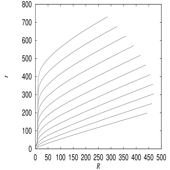
Figure 2: Trajectories of outgoing light rays in the background geometry.

The results of integrating Eq. (4) are shown in Figs. 3(a) and (b), where $\Delta\phi$ is defined as

$$\Delta\phi\equiv\frac{\phi(t,r)-\phi_{0}}{\phi_{0}}.$$ (25)

It is found that the value of the scalar field around the black hole is slightly smaller than the asymptotic value because of the underdensity of the surrounding region. Nevertheless, the scalar field as a whole is almost spatially homogeneous at each moment, in spite of the existence of the black hole. The evolution of the scalar field near the event horizon is well described by the cosmological homogeneous solution.

(a)

(b)

Figure 3: $\Delta\phi\equiv(\phi-\phi_{0})/\phi_{0}$ (a) along the world lines $R=\mbox{const}$ and on the hypersurfaces $t=\mbox{const}$.

7 Summary

We have calculated the evolution of the Brans-Dicke scalar field in the presence of a primordial black hole formed in a flat FRW universe. We have found that the value of the scalar field at the event horizon almost maintains the cosmological value at each moment. This suggests that primordial black holes “forget” the value of the gravitational constant at their formation epoch. However, it should be stressed that this result has only been demonstrated for a dust universe in which the scalar field does not appreciably affect the background curvature. It remains to be seen whether the same conclusion applies when these assumptions are dropped.

We are grateful to T. Nakamura for helpful discussions and useful comments.

References

- [1] S.W. Hawking, Commun. Math. Phys. 43, 199 (1975).
- [2] B.J. Carr, Astrophys. J. 201, 1 (1975).
- [3] J.D. Barrow, Phys. Rev. D 46, 3227 (1992).
- [4] J.D. Barrow and B.J. Carr, Phys. Rev. D 54, 3920 (1996).
- [5] B.J. Carr and C.A. Goymer, Prog. Theor. Phys. 136, 321 (1999); C.A. Goymer and B.J.Carr, Phys. Rev. D., in press.
- [6] T. Jacobson, Phys. Rev. Lett. 83, 2699 (1999).
- [7] T.M. Eubanks et al., Bull. Am. Phys. Soc., Abstract #K 11.05 (1997); C.M. Will, gr-qc/9811036.
- [8] T. Harada, T. Chiba, K. Nakao and T. Nakamura, Phys. Rev. D 55, 2024 (1997).
- [9] H. Iguchi, K. Nakao and T. Harada, Phys. Rev. D 57, 7262 (1998); H. Iguchi, T. Harada and K. Nakao, Prog. Theor. Phys. 101, 1235 (1999); Prog. Theor. Phys. 103, 53 (2000).
- [10] B.J. Carr and S.W. Hawking, MNRAS 168, 399 (1974).