X-ray reflection by photoionized accretion discs

Abstract

Calculations of X-ray reflection spectra from ionized, optically-thick material are an important tool in investigations of accretion flows surrounding compact objects. We present the results of reflection calculations that treat the relevant physics with a minimum of assumptions. The temperature and ionization structure of the top five Thomson depths of an illuminated disc are calculated while also demanding that the atmosphere is in hydrostatic equilibrium. In agreement with Nayakshin, Kazanas & Kallman, we find that there is a rapid transition from hot to cold material in the illuminated layer. However, the transition is usually not sharp so that often we find a small but finite region in Thomson depth where there is a stable temperature zone at $T\sim 2\times 10^{6}$ K due to photoelectric heating from recombining ions. As a result, the reflection spectra often exhibit strong features from partially-ionized material, including helium-like Fe K lines and edges. The reflection spectra, when added to the illuminating spectra, were fit by the publicly available constant density models (i.e., pexriv, pexrav and the models of Ross & Fabian). We find that due to the highly ionized features in the spectra these models have difficulty correctly parameterizing the new reflection spectra. There is evidence for a spurious $R-\Gamma$ correlation in the ASCA energy range, where $R$ is the reflection fraction for a power-law continuum of index $\Gamma$, confirming the suggestion of Done & Nayakshin that at least part of the $R-\Gamma$ correlation reported by Zdziarski, Lubiński & Smith for Seyfert galaxies and X-ray binaries might be due to ionization effects. However, large uncertainties in the fit parameters prevent confirmation of the correlation in the 3–20 keV energy range. Although many of the reflection spectra show strong ionized features, these are not typically observed in most Seyfert and quasar X-ray spectra. However, the data are not yet good enough to place constraints on the illumination properties of discs, as instrumental and/or relativistic effects could mask the ionized features predicted by the models.

1 Introduction

The X-ray spectra from luminous accreting black holes, both of stellar mass and in the nuclei of galaxies, generally consist of a thermal component attributed to viscous dissipation in a thin dense disc and a harder power-law component attributed to an optically-thin corona above the disc. Irradiation of the thin disc by the corona yields another component, termed the reflection spectrum. The spectral shape of this component depends in detail upon the incident coronal emission as well as the ionization state of the surface layers of the disc. Hydrogen and helium are of course highly ionized, but heavier elements such as oxygen, silicon and particularly iron may not be completely stripped of electrons and so can impart characteristic spectral features, lines and edges, into the observed spectrum. Such features can be of great importance since they carry information about the disc material, such as its ionization state and composition, as well as its motion and depth in the gravitational well of the black hole.

Initial studies of such photoionized discs have commonly assumed that the surface density is constant with depth (Ross & Fabian 1993; Matt, Fabian & Ross 1993a,b; Życki et al. 1994; Ross, Fabian & Young 1999). Constant density may be an appropriate approximation for the bulk of a radiation-pressure-supported disc. Recently, Nayakshin and colleagues (Nayakshin, Kazanas & Kallman 2000; Nayakshin & Kallman 2001; Done & Nayakshin 2001; Nayakshin 2000) have studied the situation in which the number density decreases with height in accord with hydrostatic equilibrium. Their results often show significant differences with those from the constant density calculations: the reflection spectrum in the 2–20 keV band consists mostly of a featureless spectrum from reflection by highly ionized outer gas, and a weak low ionization component from deeper recombined gas. This major difference is attributed to a thermal instability (e.g., Krolik, McKee & Tarter 1981) that can cause a sharp transition in the density and temperature profiles. However, Nayakshin et al. (2000) artificially vary the relative strength of gravity on the atmosphere (parameterized by their $A$ parameter; eq. 9) in an attempt to account for any effects by a local outflow due to heating by magnetic flares above the disc.

Here we report on our study of the reflection spectra from disc atmospheres in hydrostatic equilibrium, using the code of Ross (1978). This is a modified version of the one with which we studied constant density atmospheres (Ross & Fabian 1993). We take a complementary approach to Nayakshin et al. (2000), and investigate the response of the reflection spectrum to changes in the disc and illumination parameters. These models will be more appropriate to fit to forthcoming XMM-Newton and Chandra data. We find that the gas temperature does drop rapidly at some point within the surface, but generally the outer, more highly ionized gas just above that point emits strong lines from hydrogenic and helium-like iron. Reflection from the outer, most highly ionized gas does add a featureless component to the spectrum. Our results approximately resemble a dilute version of the constant density spectra.

The paper is organized as follows. In Section 2, we outline the changes we made to the Ross & Fabian (1993) code to include hydrostatic equilibrium. The following section (§ 3) presents the results of the calculations. In Section 4 we illustrate how the new calculations differ from earlier constant density ones. We fit simulated spectra comprised from the new models with the older constant density models in Section 5. Section 6 contains a discussion on the limitations of the code as it now stands. We discuss the implications of our results in Sect. 7, and summarize the conclusions in Section 8.

2 Computations

We model the uppermost layer of an accretion disc that is illuminated directly from above, as by local magnetic flares. This atmosphere is treated down to a Thomson depth $\tau_{\rm T}=5$, so that little of the X-ray illumination reaches the bottom of this layer without first interacting with the gas. The external illumination is assumed to have the form of a power-law spectrum with photon index $\Gamma$ (i.e., photon flux $\propto E^{-\Gamma}$) and extends from 1 eV to a sharp cutoff at 100 keV. The radiation entering the atmosphere from the disc below is in the form of an effective blackbody spectrum with total flux given by the Newtonian value [1973],

$$F_{\rm disc}=\frac{3GM\dot{M}}{8\pi R^{3}}\left[1-\left(\frac{3R_{\rm S}}{R}\right)^{1/2}\right],$$ (1)

where $M$ is the mass of the central black hole, $\dot{M}$ is the accretion rate, $R$ is the radial distance away from the black hole, and $R_{\rm S}$ is the Schwarzschild radius. (For an accretion disc extending down to $3R_{\rm S}$, the resulting efficiency is $\eta\equiv L/\dot{M}c^{2}=1/12$.) The base of the atmosphere is fixed at a vertical height above the midplane of the disc equal to the expected half-thickness of a gas-pressure dominated disc with $\alpha=0.1$ [2000],

$$H=(8.33\times 10^{3}{\rm\thinspace cm})\dot{m}^{1/5}m^{9/10}r^{21/20}\left(1-\sqrt{\frac{3}{r}}\right)^{1/5},$$ (2)

where $m=M/M_{\odot}$, $r=R/R_{\rm S}$, and $\dot{m}=\dot{M}/\dot{M}_{\rm Edd}$ ($\dot{M}_{\rm Edd}=4\pi Gm_{p}M/\eta\sigma_{\rm T}c$, where $m_{p}$ is the proton mass, is the Eddington accretion rate).

The method of treating the radiative transfer has been described by Ross & Fabian (1993). The penetration of X-rays from the external illumination is treated analytically in a one-stream approximation. The diffuse radiation in the atmosphere resulting from the impingement of the disc flux, Compton scattering of the illuminating radiation, and emission within the gas is treated using the Fokker-Planck/diffusion method of Ross, Weaver & McCray [1978] in plane-parallel geometry. The local temperature and ionization state of the gas is found by solving the equations of thermal and ionization equilibrium, so that they are consistent with the local radiation field. Hydrogen and helium are assumed to be fully ionized, while the following ionization stages of the most abundant metals are treated: C v–vii, O v–ix, Mg ix–xiii, Si xi–xv, and Fe xvi–xxvii.

The density of the gas is found from the condition for hydrostatic equilibrium. Let us denote the net upward spectral flux at height $z$ above the midplane of the disc by

$${\cal F}_{\nu}(z)=F_{\nu}(z)-X_{\nu}(z),$$ (3)

where $F_{\nu}$ is the contribution due to diffuse radiation and $X_{\nu}$ is the magnitude of the contribution due to direct inward penetration of the external illumination. In the thin-disc approximation, the equation of hydrostatic equilibrium in the vertical direction is

$$-\frac{dP_{\rm gas}}{dz}+\int_{0}^{\infty}\rho\kappa_{\nu}\frac{F_{\nu}}{c}d\nu-\int_{0}^{\infty}\rho\kappa_{\nu}\frac{X_{\nu}}{c}d\nu=\frac{GM\rho}{R^{3}}z,$$ (4)

where $P_{\rm gas}$ is the gas pressure, $\rho$ is the gas density, and $\kappa_{\nu}$ is the opacity. At interior points, the diffuse flux is given by

$$F_{\nu}=-\frac{c}{3\rho\kappa_{\nu}}\frac{du_{\nu}}{dz},$$ (5)

where $u_{\nu}$ is the spectral energy density. Therefore, except at the boundaries of the atmosphere, equation (4) simplifies to

$$-\frac{dP_{\rm gas}}{dz}-\frac{1}{3}\frac{du}{dz}-\int_{0}^{\infty}\rho\kappa_{\nu}\frac{X_{\nu}}{c}d\nu=\frac{GM\rho}{R^{3}}z,$$ (6)

where $u$ is the total energy density in diffuse radiation. Dividing through by $n_{\rm e}\sigma_{\rm T}$, where $n_{\rm e}$ is the number density of free electrons and $\sigma_{\rm T}$ is the Thomson cross section, equation (6) gives

$$\frac{dP_{\rm gas}}{d\tau_{\rm T}}+\frac{1}{3}\frac{du}{d\tau_{\rm T}}-\int_{0}^{\infty}\frac{\rho\kappa_{\nu}}{n_{\rm e}\sigma_{\rm T}}\frac{X_{\nu}}{c}d\nu=\frac{GM\rho}{n_{\rm e}\sigma_{\rm T}R^{3}}z,$$ (7)

where $\tau_{\rm T}$ is the Thomson depth inward from the surface. With helium at one-tenth the number abundance of hydrogen, the relations $P_{\rm gas}=2.3n_{\rm H}kT$, $\rho=1.4n_{\rm H}m_{\rm H}$, and $n_{\rm e}=1.2n_{\rm H}$ are used to make the dependent variable $n_{\rm H}$, the number density of hydrogen.

We use the following procedure to model the illuminated atmosphere. The solution is sought over a grid of 110 zones in Thomson depth $\tau_{\rm T}$ by 210 bins in photon energy $E$. The initial density distribution is taken to be a Gaussian with scale height equal to the half-thickness of the disc below,

$$n_{\rm H}(z)=n_{0}\exp\left[-\frac{(z-H)^{2}}{H^{2}}\right],$$ (8)

with base density $n_{0}$ chosen so that the atmosphere has the desired total Thomson depth. With the density structure fixed, the temperature structure and radiation field throughout the gas are determined as described by Ross & Fabian (1993).

This temperature structure and radiation field are then used to find an implied density structure. Starting at the current estimate for the top height of the atmosphere and assuming that the gas pressure is negligibly small above it, equation (4) is used to find the value of $n_{\rm H}$ in the uppermost zone. This density and the desired value of $\tau_{\rm T}$ at the base of the uppermost zone then establishes the height ($z$) there. Working inward through the atmosphere, equation (7) is used to find the value of $n_{\rm H}$ and the base height for subsequent zones. When the bottom zone is reached, the height implied for the base of the atmosphere, $z_{\rm base}$, is compared with the desired height $H$. The estimate for the top height of the atmosphere is adjusted and the integration inward is repeated until the proper base height, $z_{\rm base}=H$, is achieved.

With a new estimation of the density structure established, the temperature structure and radiation field throughout the gas are recalculated. The procedures for finding the density structure, the temperature structure, and the radiation field are repeated until the model converges. Our convergence condition was that all of the following must be true: a) at least 15 iterations must have been completed (this guarantees that the various ionization and recombination fronts have had time to propagate through the model), b) the fractional change in the top height from the previous iteration is less than 10^-4, c) the fractional change in the surface temperature is less than 10^-3, and d) the fractional change in the surface density is less than 10^-3. In almost all cases, the models did not require many more iterations than the 15 they were originally allocated.

3 Results

Our models require six input parameters: three describing properties of the disc, and three describing properties of the illuminating radiation. The three disc properties are the black hole mass $m$, the accretion rate $\dot{m}$, and the radius along the accretion disc $r$. The three parameters that describe the incident radiation are the photon-index of the illuminating power-law $\Gamma$, the flux $F_{x}$ (in erg cm^-2 s^-1), and the incidence angle $i$ (measured from the normal). In the following subsections we will show the results of the models varying each of the parameters in turn, deferring a detailed quantitative discussion of the results to later sections. Our canonical model, from which all variations were originated, had the following parameters: $m=10^{8}$, $\dot{m}=0.001$, $r=9$, $\Gamma=1.9$, $F_{x}=10^{15}$, and $i=\cos^{-1}(1/\sqrt{3})=54\aas@@fstack{\circ}7$.

To facilitate comparison with the results of Nayakshin et al. (2000), we also calculate their parameter $A$, where

$$A={GM\rho Hc\over R^{3}\sigma_{\rm T}n_{\rm e}F_{x}}={5.42\times 10^{20}H\over m^{2}r^{3}F_{x}}.$$ (9)

For our canonical model, $A=0.0207$. We have summarized all the models presented in this section, along with their $A$ values, in Table 1.

Table 1: A summary of the parameters used to calculate the models presented in Section 3.

Type of	$\Gamma$	$F_{x}$	$i$	$r$	$m$	$\dot{m}$	$A$	$F_{x}/F_{\rm disc}$
Model		(erg cm-2 s-1)	(degrees)
Canonical	1.9	1015	54.7	9	108	0.001	0.0207	144
Vary $\Gamma$	2.2	–	–	–	–	–	–	–
	2.1	–	–	–	–	–	–	–
	2.0	–	–	–	–	–	–	–
	1.8	–	–	–	–	–	–	–
	1.7	–	–	–	–	–	–	–
	1.6	–	–	–	–	–	–	–
Vary $F_{x}$	1.9	1016‡	–	–	–	–	0.0021	1442
	–	$5\times 10^{15{\ddagger}}$	–	–	–	–	0.0041	721
	–	$5\times 10^{14}$	–	–	–	–	0.0414	72
	–	1014	–	–	–	–	0.2068	14
Vary $i$	–	1015	20	–	–	–	0.0207	144
	–	–	80	–	–	–	–	–
Vary $r$	–	–	54.7	4	–	–	0.0799	40
	–	–	–	6	–	–	0.0424	62
	–	–	–	8	–	–	0.0256	110
	–	–	–	10	–	–	0.0171	185
	–	–	–	12	–	–	0.0122	289
	–	–	–	16	–	–	0.0071	604
	–	–	–	18‡	–	–	0.0057	824
Vary $m$	–	–	–	9	109‡	–	0.0016	1442
	–	–	–	–	107	–	0.2604	14
Vary $\dot{m}$	–	–	–	–	108	0.1†	0.8428	1.4
	–	–	–	–	–	0.05†	0.4214	2.9
	–	–	–	–	–	0.01	0.0328	14
	–	–	–	–	–	0.005	0.0285	29
	–	–	–	–	–	0.0025	0.0248	58
	–	–	–	–	–	0.0005	0.0180	288

^† utilized radiation pressure boundary conditions

^‡ calculated with a $\tau_{T}=10$ deep atmosphere

3.1 Varying the photon index

In the top panel of Figure 1, we present our calculated reflection spectra for six values of the photon index $\Gamma$.

Figure 1: Top: Reflection spectra for models where the photon-index of the illuminating power-law has been varied. All the other parameters have the same values as in the canonical model, so all these models have the value of $A=0.0207$. The spectra have been offset vertically for clarity. The dotted curve shows the spectrum from the disc that is incident on the base of the atmosphere. Bottom: The temperature of the atmosphere as a function of Thomson depth for three different values of $\Gamma$. The harder the spectrum, the deeper into the atmosphere it ionized, and the sharper the thermal transition.

The bottom panel shows how the temperature of the atmosphere varies with Thomson depth for three different values of $\Gamma$. The harder spectra ionize further into the slab than the softer ones, and have a sharper thermal transition. This results in a highly ionized and reflective spectrum as is seen in the top panel in Figure 1. The softer illuminating spectra result in a much more complex reflection spectrum, exhibiting features from a variety of ionization states.

To emphasize the properties of the Fe K$\alpha$ line, we present in Figure 2 the reflection spectra plotted between 1 and 10 keV.

Figure 2: The same reflection spectra as shown in Fig. 1, but plotted between 1 and 10 keV to emphasize the features of the Fe K$\alpha$ line. Again, the spectra have been offset vertically for ease of presentation. The dotted vertical lines show the positions of the iron lines at 6.4, 6.7 and 7.0 keV. The ionized Fe lines at 6.7 and 7.0 keV are found in the reflection spectra, irrespective of the photon-index of the illuminating continuum.

The Fe K$\alpha$ line is only barely visible when the illuminating spectrum is very hard, and then becomes more pronounced as the incident power-law softens. However, we find that when the disc is highly illuminated (as it is in all our models) at no point does a neutral Fe line at 6.4 keV become prominent. The Fe line complex is made up almost entirely from the ionized lines at 6.7 and 7.0 keV.

3.2 Varying the illuminating flux

Next, we consider models where the illuminating flux is varied over two orders of magnitude. Figure 3 shows the reflection spectra and the temperature structure for some of these models.

Figure 3: Top: Reflection spectra for models where the illuminating flux has been varied. All the other parameters have the same values as in the canonical model. The spectra have been offset vertically for clarity. The dotted curve shows the spectrum from the disc that is incident on the base of the atmosphere. Since the models with $F_{x}=10^{16}$ and $5\times 10^{15}$ erg cm^-2 s^-1 ionize through 5 Thomson depths, they were calculated with the atmosphere extending down to $\tau_{\rm T}=10$. The reflection spectrum for the least intense illuminating flux is the only one with many ionized features. Bottom: The temperature of the atmosphere as a function of Thomson depth for three different values of $F_{x}$. The least intense radiation field has hardly any mid-temperature shoulder and does not ionize very far into the atmosphere. In all cases, the units of $F_{x}$ are erg cm^-2 s^-1.

The illuminating radiation fields with $F_{x}=10^{16}$ and $5\times 10^{15}$ erg cm^-2 s^-1 ionize through five Thomson depths so these models were calculated with the atmosphere extending down to $\tau_{\rm T}=10$. As the illuminating flux is wound down, the temperature transition becomes much sharper, and moves closer to the surface of the atmosphere. Indeed, the reflection spectrum for the model with $F_{x}=10^{14}$ erg cm^-2 s^-1, is the only one out of the four to show many ionized lines.

3.3 Varying the incidence angle

Our canonical model assumes as a crude approximation to isotropic radiation that the incident photons are striking the atmosphere at an incidence angle of $i=54\aas@@fstack{\circ}7$, such that $\mu=\cos i=1/\sqrt{3}$. Figure 4 shows the results when we change the angle of incidence to 20^∘ and to 80^∘. The incidence angle is measured with respect to the normal, so that large angles correspond to grazing incidence.

Figure 4: Top: Reflection spectra for models where the incidence angle of the radiation has been varied. All the other parameters have the same values as in the canonical model. The spectra have been offset vertically for clarity. The dotted curve shows the spectrum from the disc that is incident on the base of the atmosphere. Bottom: The temperature of the atmosphere as a function of Thomson depth for three different values of $i$. The most direct radiation ionizes deeper into the atmosphere.

The results are not surprising. The radiation that is more directly illuminating the atmosphere ionizes deeper into the slab than the radiation that has a grazing incidence. However, at these high flux levels there is little effect on the emergent reflection spectrum.

3.4 Varying the radius

In Figure 5 we have plotted the reflection spectra and the temperature structure for models at different radii along the accretion disc, but with all other parameters held at their canonical values (e.g., $F_{x}=10^{15}$ erg cm^-2 s^-1).

Figure 5: Top: Reflection spectra for models where the radius at which the illumination occurs has been varied. All the other parameters have the same values as in the canonical model. The spectra have been offset vertically for clarity. The dotted curve shows the spectrum from the disc (when $r=4$) that is incident on the base of the atmosphere. The model with $r=18$ ionizes through five Thomson depths, so a thicker atmosphere with $\tau_{\rm T}=10$ was used for this model. The spectra are more ionized as the radius increases, reflecting the decreasing the density of the disc (which is a result of the increasing height). Bottom: The temperature of the atmosphere as a function of Thomson depth for three different values of $r$.

As the radius increases, the height of the disc increases (eq. 2) which drops the density, and the amount of soft flux emitted by the disc decreases (eq. 1). As a result of the decreasing density, the atmosphere is more ionized as the radius increases. In fact, when $r=18$ the radiation ionized through 5 Thomson depths, and so a $\tau_{\rm T}=10$ layer was used for this model.

3.5 Varying the black hole mass

In Figure 6 we plot reflection spectra for the cases when the black hole mass has been increased to 10⁹ M_⊙ and decreased to 10⁷ M_⊙.

Figure 6: Top: Reflection spectra for models where the black hole mass has been changed. All the other parameters have the same values as in the canonical model. The spectra have been offset vertically for clarity. The dotted curve shows the spectrum from the disc (when $m=10^{7}$) that is incident on the base of the atmosphere. When $m=10^{9}$, the density of the disc was so low that the incident radiation ionized through 5 Thomson depths, and so a deeper layer with $\tau_{\rm T}=10$ was used for this model. These reflection spectra show the differences of the changing density with black hole mass. Bottom: The temperature of the atmosphere as a function of Thomson depth for three different values of $m$.

The model with the lowest black hole mass is not able to ionize as far into the atmosphere as compared with the ones with larger masses. This is because the disc becomes thinner as the black hole mass decreases (see eq. 2), so the top layer of the atmosphere is actually much denser in the low $m$ cases than in the high $m$ cases. Specifically, in the $m=10^{9}$ model, we find the density at the top of the atmosphere to be $\sim 10^{8}$ cm^-3, while in the $m=10^{7}$ model, this density has increased to $\sim 6\times 10^{9}$ cm^-3. Therefore, the exact same ionizing spectrum cannot penetrate as far into the layer. Furthermore, the larger density will increase the cooling rates which will contribute to the temperature transition occurring closer to the surface. As a result, the reflection spectrum for the smaller black hole masses show stronger features from neutral reflection (but still show ionized Fe K$\alpha$ lines). For the $m=10^{9}$ model an atmosphere with $\tau_{\rm T}=10$ had to be used to fully realize this situation.

As is discussed in Sect. 6, our code has difficulty if the thermal transition occurs at a Thomson depth $\la 0.2$. As the black hole mass decreases, the disc becomes denser, so the same amount of ionizing flux will not penetrate as far. Therefore, we cannot model systems with black hole masses much smaller than 10⁷ M_⊙ without ramping up the illuminating flux. In this section we are only interested in comparing the results when one parameter is varied at a time, so using $F_{x}=10^{15}$ erg cm^-2 s^-1 restricts us to a limited range of black hole mass.

3.6 Varying the accretion rate

We have varied the accretion rate over three orders of magnitude, and the results are displayed in Figure 7. As the accretion rate is increased, the amount of soft disc radiation increases. However, our boundary condition, the height $H$ of the base of the atmosphere, is appropriate for only a gas-pressure dominated disc, and so it does not rise as rapidly with $\dot{m}$ as is needed to compensate for the increasing radiation pressure. Indeed, increasing the accretion rate much beyond $\dot{m}=0.01$ results in a large density inversion in the lower regions of the atmosphere, as the gas has to push downwards to assist the weak gravity (due to low $z/r$) and balance the strong radiation pressure from the thermal disc emission. Therefore, for $\dot{m}=0.05$ and 0.1 radiation pressure boundary conditions from Merloni et al. (2000) were used instead of the gas pressure dominated ones.

Figure 7: Top: Reflection spectra for models where the accretion rate has been varied. All the other parameters have the same values as in the canonical model. The spectra have been offset vertically for clarity. The dotted curve shows the spectrum from the disc (when $\dot{m}=0.005$) that is incident on the base of the atmosphere. The spectra for $\dot{m}=0.05$ and 0.10 were calculated with the radiation pressure dominated boundary conditions from Merloni et al. (2000). Bottom: The temperature of the atmosphere as a function of Thomson depth for three different values of $\dot{m}$. The small temperature increase at high Thomson depth in the $\dot{m}=0.05$ model is a result of the large soft flux emanating from the disc.

We find that there is not much difference between the reflection spectra as the accretion rate varies. This result indicates that, aside from the height of the disc, the internal structure of the atmosphere is not greatly affected by changing the accretion rate. However, the soft flux from the disc does increase with $\dot{m}$ and becomes comparable to the illuminating flux when $\dot{m}\approx 0.05$. At this point, a strong O v recombination line at about 0.05 keV is observed in the spectra. Also, the bremsstrahlung flux between 0.01 and 0.1 keV increases with $\dot{m}$, as the strong soft disc radiation is thermalized by the ionized gas. However, the hard X-ray spectra above 1 keV displays little variation as the accretion rate is changed.

4 Comparison with previous work

Previous studies of accretion disc atmospheres that incorporated hydrostatic balance have been carried out by Raymond (1993), Ko & Kallman (1994), Różańska & Czerny (1996), and Różańska (1999). The first two papers dealt with the ultraviolet and soft X-ray emission from Low-Mass X-ray Binaries, while the next two, although dealing with active galactic nuclei (AGN), did not include detailed calculations of the radiative transfer of spectral features. Therefore, it is not possible to compare our results with these earlier papers.

Recently, Nayakshin et al. (2000) have calculated the X-ray reflection spectrum from an ionized AGN accretion disc atmosphere. Their calculations included a comparable amount of physics as ours, so in principle a comparison between the two approaches could be made. However, the reflection spectra presented in their paper were calculated by artificially varying the $A$ parameter while keeping all the other parameters fixed. This was done to try to account for local dynamical effects that might occur if the disc was illuminated by bright magnetic flares (e.g., Galeev, Rosner & Vaiana 1979; Haardt, Maraschi & Ghisellini 1994; Svensson 1996). In our calculations, $A$ is fixed once we have chosen all the parameters. As a result, there are no common calculations between the two approaches and a comparison cannot be made at this time.

The results of these new calculations are more complicated to interpret than earlier constant density ones where the reflection spectrum depends only on the ionization parameter of the gas. Here, the ionization parameter changes with depth as the density changes. Therefore, different regions of the reflection spectrum will arise from different depths within the layer. The temperature and ionization structures of our canonical model, plus the strengths of the processes which setup those structure, are shown in Figure 8. The top panel plots the heating and cooling rates for various processes over the transition region for the canonical model (see the caption for identification of the various curves). The bottom panel plots both the Fe ionization structure and the Compton temperature over the same region.

Figure 8: Top: (H)eating and (C)ooling rates for various processes in the canonical model plotted versus the range of Thomson depth that covers the transition region. The solid black curve denotes the gas temperature. The rates are denoted as follows: red curves=heating processes, blue curves=cooling processes, dotted=Compton processes, short dash=bremsstrahlung, long dash=recombination, dot-short dash=photoelectric heating/line cooling, and dot-long dash=three-body. Bottom: The dark solid line plots the Compton temperature versus Thomson depth. The other curves illustrate the Fe ionization structure over this region. The long dashed curve denotes completely ionized iron, the solid curve closer to the surface shows hydrogenic iron, the short dashed line plots helium-like iron, the dotted curves correspond to Fe xvii–xxv, and the solid curve near the bottom of the transition zone plots “neutral” Fe xvi.

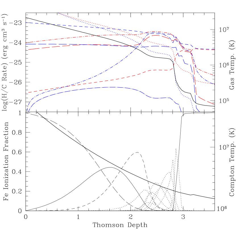
At the top of the atmosphere, Compton heating and cooling are the dominant processes, Fe is completely ionized, and the gas temperature is comparable to the Compton temperature. However, as we move into the layer, the Compton temperature immediately starts dropping since ionizing photons are being reflected by the ionized top and are not making it further into the layer. Hydrogenic iron begins to build up and is the dominant species at a Thomson depth of about 1.4. Note that the temperature plateau has not yet been reached, but the gas is hotter then the Compton temperature. At this point Compton cooling is surpassed by bremsstrahlung cooling because of the increasing density. This cooling quickly exceeds the Compton heating rate, and the gas temperature takes its first sharp turn downwards. Helium-like Fe quickly builds up to be the dominant species (it is the line at 6.7 keV from this species that is the most prominent line in the reflection spectrum) just before $\tau_{\rm T}=2.2$. The plateau is still not reached yet, but photoelectric heating from the quickly recombining ions has become the dominant form of heating. Free-free cooling is still dominating the cooling, but line cooling is quickly gaining and dominates just past a Thomson depth of 2.3. This is when the stable temperature plateau is found. It is kept stable by the balance of photoelectric heating of the various ionization states of Fe and its subsequent line cooling plus free-free cooling. Finally, the ionizing photon density drops to the point where everything can recombine and we are left with neutral material with free-free heating and cooling dominating.

5 Fitting the new models with constant density ones

Previous fits to X-ray spectra that employed reflection models were limited to ones where the density was assumed to be constant within the atmosphere. The most widely used publicly available models have been the pexriv (for ionized reflection) and pexrav (for neutral reflection) models of Magdziarz & Zdziarski (1995) that are included as part of the xspec spectral fitting package. The constant density models of Ross & Fabian (1993) have also been used to fit X-ray spectra (e.g., Ballantyne, Iwasawa & Fabian 2001). Now that variable density models are available, it is instructive to fit them with the older, constant density ones. This exercise will illustrate the differences between the variable density models and constant density ones. It will also point out possible errors in analysis that could have been made as a result of fitting constant density models to spectral data. To isolate these effects, we have not added any further spectral complexity (i.e., warm absorbers, soft excess, or neutral absorption) to the model spectra.

We begin by generating simulated spectra using the results of the calculations. This is accomplished by first adding the reflection spectrum to the illuminating spectrum (so that the reflection fraction, $R$, is unity), and then using the ‘fakeit’ command in xspec v.11 to create simulated spectra with a certain exposure time. To examine the results of fitting the models over different energy ranges, we used the RXTE and the ASCA SIS0 response matrices from our study of Ark 564 (Ballantyne et al. 2001) to produce two different versions of each simulated spectrum. The normalization of the models and the exposure times for each spectrum-response matrix pair are shown in Table 2, and were chosen so that there were at least 20 counts per bin (which allows the use of the $\chi^{2}$ statistic as a goodness of fit parameter). The normalizations are so small because the model predicts flux in units of emitting area. The values chosen here are typical of ones that are obtained when fitting real data.

Table 2: Normalizations and exposure times assumed for the simulated spectra that are analyzed in this section.

	RXTE		ASCA
$\Gamma/F_{x}^{a}$	$\log$(Norm.b)	Exp. Timec	$\log$(Norm.b)	Exp. Timec
2.2	$-27$	200	$-25$	175
2.1	$-27$	175	$-25$	150
2.0	$-27$	100	$-25$	100
1.9	$-27$	100	$-25$	100
1.8	$-27$	100	$-25$	100
1.7	$-27$	100	$-25$	100
1.6	$-27$	100	$-25$	100
$10^{16}$	$-27$	100	$-26$	100
$5\times 10^{15}$	$-27$	100	$-25$	100
$5\times 10^{14}$	$-26$	100	$-25$	400
$10^{14}$	$-26$	100	$-24$	200

^a units of erg cm^-2 s^-1

^b units of photons cm^-2 s^-1

^c units of kiloseconds

We then fit the spectra using the chosen model over three different energy ranges: 3–20 keV (using the RXTE response matrix), 0.5–10 keV and 1–10 keV (using the ASCA SIS0 response matrix). It is worth pointing out that because of the randomness in generating these simulated spectra (since ‘fakeit’ includes random photon noise in each spectrum), the actual numerical values of the fits are not solid results. However, trends in the fits and whether or not a spectrum is fit ‘well’ or fit ‘poorly’ are valid results, and can be used to draw conclusions.

We first fit the pexriv and pexrav models to our variable density models which have had the photon index varied from 2.2 to 1.6 (the other model parameters are the same as the canonical model; see Table 1). As seen in Fig. 1, these spectra cover the range from highly ionized and featureless ($\Gamma=1.6$), to ones which have more pronounced spectral features ($\Gamma=2.2$). Since pexriv and pexrav do not include any line emission, each fit included a Gaussian to model the Fe K$\alpha$ line. The central energy of the Gaussian was fixed at 6.7 keV  which is the energy of the Fe K$\alpha$ line in our model spectra, the width was fixed at 0.5 keV, and the normalization was allowed to vary. It is worth pointing out that in these models there is no physical connection between the strength and energy of the Fe K$\alpha$ line and the edge that appears in the continuum. This is one of the chief weaknesses of using the pexriv+gauss or pexrav+gauss models to fit data which includes an Fe K$\alpha$ line. The continuum parameters were set as follows: cutoff energy of power-law=400 keV, inclination angle=30^∘, abundances=solar, and (pexriv only) temperature of disc=10⁶ K. The results of these fits are shown in Table 3.

Table 3: Results of fitting the pexriv and pexrav models to our new models (incident+reflected). These models were computed with $m=10^{8}$, $\dot{m}$=0.001, $F_{x}=10^{15}$ erg cm^-2 s^-1, $r=9$, $i=54\aas@@fstack{\circ}7$, and had the photon index varied from 2.2 to 1.6. A Gaussian line was included in all fits to model the Fe K$\alpha$ complex. The energy of the line was fixed at 6.7 keV and the intrinsic width was fixed at 0.5 keV; however, the normalization was free to vary. Further details on the parameters are discussed in the text.

	RXTE (3–20 keV)						ASCA (0.5–10 keV)						ASCA (1.0–10 keV)
	pexriv- 40 dof			pexrav- 41 dof			pexriv- 642 dof			pexrav- 643 dof			pexriv- 608 dof			pexrav- 609 dof
$\Gamma_{model}$	$R$	$\Gamma$	$\chi^{2}$	$R$	$\Gamma$	$\chi^{2}$	$R$	$\Gamma$	$\chi^{2}$	$R$	$\Gamma$	$\chi^{2}$	$R$	$\Gamma$	$\chi^{2}$	$R$	$\Gamma$	$\chi^{2}$
2.2	0.04	2.21	50	0.0	2.20	50	1.63	2.39	770	1.75	2.39	771	1.38	2.41	628	3.27	2.43	628
2.1	0.0	2.21	44	0.0	2.20	44	0.52	2.22	744	0.70	2.22	746	0.96	2.24	673	1.1	2.23	677
2.0	0.0	2.00	42	0.0	1.99	42	0.88	2.13	671	1.3	2.13	672	0.68	2.12	588	2.1	2.16	611
1.9	0.0	1.93	40	0.0	1.93	40	0.24	1.99	681	0.31	1.99	683	0.17	1.98	615	0.47	2.00	621
1.8	0.17	1.82	55	0.16	1.83	56	0.39	1.90	644	0.69	1.91	652	0.56	1.92	595	0.70	1.90	605
1.7	0.06	1.70	35	0.01	1.68	35	0.0	1.80	826	0.0	1.80	826	0.11	1.81	788	0.0	1.80	788
1.6	0.0	1.61	41	0.0	1.60	41	0.24	1.71	701	0.06	1.70	705	0.0	1.68	651	0.0	1.68	651

The first noticeable result from the fits is that, in almost all cases, the pexriv and pexrav models do a good job fitting the spectra in the 3–20 keV range: the $\chi^{2}$ of the fit is low and the derived value of the photon index is close to the true value. This is due to the fact that, aside from the Fe K$\alpha$ line and its associated edge, the spectra are relatively smooth and featureless in this region. Of course, the model can fit both the line and the edge, so that the $\chi^{2}$ is quite low. Even though the pexrav model is appropriate only for neutral reflection, it still provides a good fit to the simulated data. This might be because the resolution of RXTE is poor enough that the difference between a neutral and an ionized Fe edge cannot be distinguished in noisy data, or the Fe K$\alpha$ normalization was adjusted to help in the fitting. Also, the fits tend to give much lower reflection fractions than the true value of $R$ (which is unity). Furthermore, the 1-$\sigma$ errors on the derived reflection fraction are quite large, which suggests that the lack of features in this spectral region, combined with the poor resolution of RXTE, makes it difficult to constrain the amount of reflection in a spectrum (this is also true for the Ross & Fabian (1993) models; see Table 5).

Moving to the ASCA energy ranges, we find that both the pexriv and the pexrav models have greater difficulty providing adequate fits to the data in the 0.5–10 keV energy range: often the value of $\Gamma$ is highly overestimated. This behaviour also persists in the 1–10 keV region. Fig. 1 shows that below about 2 keV the reflection spectrum begins to steepen. The pexriv and pexrav models do not have enough spectral curvature to account for this change and therefore must steepen the power-law in order to fit these low energy data. As a result the model will underestimate the spectrum at the high energy end, and must increase the amount of reflection to increase the quality of the fit. The ionization state of the reflection spectrum increases as $\Gamma$ decreases and therefore the amount of reflection the model requires in order to obtain a best-fit will decrease. Ignoring the data below 1 keV will remove some of the steepening, and the results obtained from pexriv and pexrav improve slightly. The above results show that pexriv and pexrav cannot adequately describe a reflection spectrum that arises from a highly ionized disc.

We then proceeded to fit the simulated spectra with the constant density models of Ross & Fabian (1993). These models, of course, contain the same atomic and ionization physics as the ones presented in this paper. Along with the models with the different values of $\Gamma$, we also fit simulated spectra for the models with differing amounts of illuminating flux (and $\Gamma=1.9$). The spectra were fit two different times: first, with the reflection fraction of the model fixed at unity (to investigate the dependence on the ionization parameter $\xi=4\pi F_{x}/n_{\rm H}$), and, second, when the reflection fraction was allowed to be fit. The results of the fits are presented in Tables 4 and 5, respectively.

Table 4: Results of fitting the constant models of Ross & Fabian (1993) to our new models (incident+reflected). The models in the top part of the table were computed with $m=10^{8}$, $\dot{m}$=0.001, $F_{x}=10^{15}$ erg cm^-2 s^-1, $r=9$, $i=54\aas@@fstack{\circ}7$, and had the photon index varied from 2.2 to 1.6. The models in the bottom part of the table were computed with $\Gamma=1.9$, and had the illuminating flux varied (all other parameters were unchanged). The reflection fraction in the constant density models was fixed at unity. For more details see the text.

	RXTE (3–20 keV)			ASCA (0.5–10 keV)			ASCA (1.0–10 keV)
$\Gamma_{model}/F_{x}^{a}$	$\log\xi$	$\Gamma$	$\chi^{2}/42$	$\log\xi$	$\Gamma$	$\chi^{2}/644$	$\log\xi$	$\Gamma$	$\chi^{2}/610$
2.2	3.80	2.11	51	4.50	2.26	804	3.83	2.23	629
2.1	4.17	2.11	47	4.70	2.12	757	4.28	2.13	673
2.0	3.91	1.91	46	6.0	1.99	671	3.94	2.02	598
1.9	3.99	1.86	44	4.90	1.85	678	4.29	1.89	613
1.8	4.10	1.72	54	4.51	1.71	650	4.05	1.75	606
1.7	3.73	1.59	37	4.59	1.58	851	4.72	1.58	815
1.6	4.11	1.51	44	4.71	1.50	898	5.02	1.50	717
$10^{16}$	4.47	1.86	40	5.12	1.81	660	4.20	1.86	628
$5\times 10^{15}$	4.21	1.84	42	4.83	1.86	812	4.05	1.89	703
$5\times 10^{14}$	3.92	1.80	38	4.97	1.87	770	4.05	1.91	675
$10^{14}$	3.72	1.77	34	4.36	1.92	887	3.67	1.93	729

^a units of erg cm^-2 s^-1

Turning our attention to the fits where the reflection fraction, $R$, was fixed at its true value of one, we find some interesting results. First, as with the pexriv and pexrav model, the best fits in a statistical sense were found in the 3–20 keV RXTE energy range. As before, in this region there are only a few spectral features, so it easier for models to fit the data. Note that this is quite a general result. To differentiate between different models, or be confident about the model parameters, it is preferable to fit data over an energy range where there will be spectral features to fit against. In the three different energy ranges considered in this experiment, we often find quite different values for $\xi$. This is an important point to keep in mind when doing spectral fitting. However, while the fits may be acceptable in a $\chi^{2}$ sense in the RXTE energy range, the derived values of the photon index are consistently low. The fits are quite poor in the 0.5–10 keV energy range, but do improve in the 1–10 keV band. The computed values of $\Gamma$ are closer to the true values, but still show erratic behaviour.

These results drive home the point that the new hydrostatic models are comprised of emission from regions with different ionization parameters. The ionization parameters that are found are, broadly speaking, fairly high and quite variable. Therefore, trying to fit the spectra with a model that has only one ionization parameter will generally lead to an average value of $\xi$ or one which is from the dominant component in the spectrum. In these models, the most significant spectral feature is from the Fe K$\alpha$ line of helium-like Fe xxv at 6.7 keV but it is weakened and broadened due to Compton scattering of the line photons. This line is prominent in constant density models at values of $\xi$ above a few thousand (Ross et al. 1999). Since this line is also prominent in the simulated spectra, values of $\xi$ greater than a few thousand are typically found by the fits. This illustrates the difficulty in fitting a single ionization parameter model to a situation which has a mixture of ionization states.

Table 5: Same as Table 4, but allowing the reflection fraction to be fit.

	RXTE (3–20 keV)				ASCA (0.5–10 keV)				ASCA (1.0–10 keV)
$\Gamma_{model}/F_{x}^{a}$	$\log\xi$	$\Gamma$	$R$	$\chi^{2}/41$	$\log\xi$	$\Gamma$	$R$	$\chi^{2}/643$	$\log\xi$	$\Gamma$	$R$	$\chi^{2}/609$
2.2	3.50	2.17	0.53	50	3.05	2.23	0.26	669	3.23	2.24	0.35	596
2.1	3.71	2.18	0.29	45	3.02	2.13	0.15	695	3.05	2.14	0.17	655
2.0	3.60	1.97	0.32	45	4.96	1.90	9.9	653	4.14	1.95	9.9	587
1.9	3.21	1.94	0.14	41	4.92	1.85	0.93	678	4.26	1.90	0.78	612
1.8	4.19	1.63	9.8	54	4.54	1.78	0.49	646	4.00	1.81	0.46	599
1.7	3.09	1.69	0.15	35	5.03	1.75	0.13	828	3.40	1.78	0.05	791
1.6	3.80	1.62	0.03	43	2.65	1.67	0.03	700	2.70	1.67	0.02	655
$10^{16}$	4.47	1.86	1.06	40	6.0	1.87	0.33	653	4.10	1.93	0.22	615
$5\times 10^{15}$	4.25	1.83	1.33	42	4.56	1.75	4.5	766	4.15	1.86	1.7	696
$5\times 10^{14}$	3.58	1.86	0.26	36	4.52	1.73	9.9	734	2.65	1.95	0.20	637
$10^{14}$	3.03	1.86	0.21	29	4.40	1.80	9.9	841	2.65	1.96	0.31	619

^a units of erg cm^-2 s^-1

When the reflection fraction is allowed to vary, the quality of the fits increases significantly. In the ASCA energy band, a similar relationship between $R$ and $\Gamma$ to the one seen using the pexriv and pexrav model is observed. Finally, this exercise emphasizes that the new hydrostatic reflection models can be qualitatively described as diluted versions of the constant density ones.

5.1 The $\mn@boldsymbol{R}$–$\mn@boldsymbol{\Gamma}$ correlation

Zdziarski, Lubiński & Smith (1999) have fit Ginga spectra of Seyfert galaxies and X-ray binaries with the pexrav model, and found that the amount of reflection correlated with the photon index. While this was initially interpreted as a possible physical correlation due to disc-corona feedback effects, it now seems likely that much of this correlation is a result of systematic errors in the standard data fitting procedures (e.g., Vaughan & Edelson 2001; Chiang et al. 2001; Nandra et al. 2000). However, recent work by Done & Nayakshin (2001) suggested that ionization effects might also contribute to the observed correlation. This may be expected as it is difficult to distinguish in data the difference between a highly-ionized disc which is strongly reflective and a disc which is more neutral but weakly reflective. Done & Nayakshin (2001) employed a Ginga response matrix, and found a $R$–$\Gamma$ correlation when fitting the models of Nayakshin et al. (2000) with pexriv.

Although there is some scatter we find similar trends in the ASCA bands when using all three constant density models. The reason for this was explained in the previous section and of course was due to ionization effects. Therefore, we can conclude that perhaps part of the $R$–$\Gamma$ correlation is due to the effects of ionized features in the reflection spectrum.

6 Limitations of current models

The greatest uncertainty in the calculations presented in this paper is the choice for the lower boundary condition of the layer. We have chosen to match the bottom height of the atmosphere to the expected thickness of a gas-dominated disc. Alternatively, Nayakshin et al. (2000) matched the total pressure at the bottom of the atmosphere, but had to assume the pressure followed a Gaussian drop-off from the disc midplane. Both choices are equally valid (or equally invalid), as the true physical structure and extent of accretion discs are not well constrained. The choice of a gas-dominated boundary condition limits the applicability of the models to systems with $\dot{m}\approx 0.001$ at small radii, or with higher accretion rates at larger radii. These limits can be increased if we let a large amount of accretion power be dissipated in the corona (Svensson & Zdziarski 1994).

The significant computational limitation with our current code is that the illuminating radiation must have a certain amount of ionizing power. In the context of the $A$ parameter of Nayakshin et al. (2000), this limitation translates into a maximum $A$ value ($\approx 1$). The difficulties are due to the thermal transition occurring too close to the surface of the atmosphere (say, $\tau_{\rm T}\la 0.2$). When this situation arises, the majority of the gas in the atmosphere is either fully or partially recombined, and, as the model relaxes, a weak ionization front propagates inwards. It is difficult for the code to get radiation out past the front since the optical depth is so high (it is much easier when the gas is mostly ionized and the gas recombines from the inside outwards). Moreover, in these situations, the transition zone occurs in an optically-thin region, and our diffusion treatment for radiative transfer becomes inappropriate. In these cases, it is likely that the reflection spectrum will be dominated by mainly neutral reflection features (much like the ones produced by constant density models with low ionization parameters).

7 Discussion

The reflection spectra presented in Sect. 3 show that, for highly illuminated discs, ionized features are quite common over a wide range of parameters. However, analyses of ASCA data of samples of Seyfert 1 galaxies (Nandra et al. 1997a) and quasars (George et al. 2000) show that ionized Fe K$\alpha$ lines are unusual, if not rare (but see Reeves & Turner 2000). Typical values of $\Gamma$ for these objects are around 1.9 or 2.0, and, by Fig. 1, we see that ionized Fe lines are predicted by the models for these values of the photon index. There are a number of possible explanations for this discrepancy. One important consideration is that because of low signal-to-noise data (especially for distant quasars), there is usually a significant uncertainty in measuring the energy of the Fe K$\alpha$ line. Often it is difficult to rule out an ionized line. Second, if the line emission is originating from material within a dozen or so Schwarzschild radii from the central black hole, then gravitational redshifting will be important, and an ionized line could be shifted so that it would appear neutral. There are also possible physical explanations for this result. Perhaps most discs are weakly illuminated, denser, or they are being irradiated at large incidence angles. In these cases, it is more likely that purely neutral reflection will occur. We will have to await high signal-to-noise spectral data in the region around the Fe K$\alpha$ line before these possible explanations can be tested.

Another interesting result from the calculations is that highly ionized, featureless reflection spectra arise only when the photon index of the illuminating power-law is less than 1.7. If simple constant density reflection models are fit to such a spectrum (when it has been added to the power-law component), they will lead to an underestimate in the strength of the reflection component in the sum. This is a possible explanation for the low reflection fractions that have been observed in Galactic Black Hole Candidates (GBHCs), when they are in their low/hard states (Gierliński et al. 1997; Done & Życki 1999). In this case, there would be no need to appeal to a two-phase accretion flow to explain the observations.

Nayakshin & Kallman (2001) and Nayakshin (2000) presented evidence that X-ray reflection results from reprocessing of radiation from magnetic flares in the corona. The basis for this conclusion was that the models of Nayakshin et al. (2000) predict that the equivalent width of the neutral Fe K$\alpha$ line decreases as the illuminating flux increases (as long as $F_{x}\gg F_{\rm disc}$, a requirement for the magnetic coronal models). They compare this result to the observed trend of decreasing Fe K$\alpha$ equivalent width with X-ray luminosity (the “X-ray Baldwin effect”; Iwasawa & Taniguchi 1993; Nandra et al. 1997b; Reeves & Turner 2000), and conclude that this is strong evidence for the magnetic flare model as compared to the lamppost model, which did not show this trend (since $F_{x}\ll F_{\rm disc}$). Again, these coronal models had the relative strength of gravity on the atmosphere artificially increased by a certain factor. From Fig. 3, we see that, as we increase $F_{x}$ over two orders of magnitude (the same range as Nayakshin 2000), the equivalent width of the Fe K$\alpha$ line drops slightly. However, it does not go to zero, and it is unclear whether the line would disappear if the illuminating flux continued to increase. We do not disagree that magnetic flares are a good model for the origin of the hard X-ray emission in AGN, but the X-ray Baldwin effect is not a good test for such a model. The Fe K$\alpha$ equivalent width is observed to drop once the 2–10 keV luminosity surpasses $\sim 10^{45}$ erg s^-1 (e.g., Nandra et al. 1997b). If these high luminosity objects have similar black hole masses as their lower luminosity cousins, then their higher luminosity might be caused by a higher accretion rate (perhaps above $\dot{M}_{\rm Edd}$). At such high rates, the accretion disc will be puffed up significantly due to the large radiation pressure from within. In these cases, it is likely there will not be an optically-thick surface for X-ray reprocessing, and the Fe K$\alpha$ line will not appear in an X-ray spectrum.

Narrow-Line Seyfert 1 Galaxies (NLS1s; Osterbrock & Pogge 1985) are an interesting sub-class of AGN with unusual X-ray properties (Brandt 1999; Leighly 1999a; Leighly 1999b; Vaughan et al. 1999b). These objects exhibit extreme X-ray variability, a strong soft excess, and steep spectra in both the soft and hard X-ray bands. There are indications from ASCA data that some of these object show ionized features in their spectra (Turner, George & Nandra 1998; Vaughan et al. 1999a; Ballantyne et al. 2001). As discussed in Sect. 6, our code has difficulty computing the structure of a weakly ionized atmosphere (such as one would get when $\Gamma\ga 2.3$) without increasing the illuminating flux to compensate for the lack of ionizing photons. In Figure 9 we show the reflection spectrum and the temperature structure for a canonical-like model with $\Gamma=2.5$ and with the illuminating flux increased to $3\times 10^{15}$ erg cm^-2 s^-1.

Figure 9: Top: Reflection spectrum of a model with $\Gamma=2.5$ and $F_{x}$ increased to $3\times 10^{15}$ erg cm^-2 s^-1. All the other parameters are the same as the canonical model. The dashed line shows the illuminating continuum, and the dotted line denotes the soft disc flux incident on the bottom of the atmosphere. The reflection spectrum shows a strong He-like Fe line at 6.7 keV. Bottom: The temperature of the atmosphere as a function of Thomson depth for the $\Gamma=2.5$ model. The temperature increase over the first 0.1 of a Thomson depth is due to photoelectric heating from the copious amounts of recombined Fe.

The temperature structure of the model shows that the atmosphere is relatively cool and barely heats up to just over a million degrees (due to photoelectric heating of the recombined Fe ions), before actually dropping to just under a 10⁶ K at the surface. The illuminating spectrum has little ionizing power, so that the Compton temperature is low enough that the thermal instability is completely skipped and the temperature falls smoothly with depth. As a result, the reflection spectrum shows plenty of features from gas at a number of different ionization states including a strong He-like Fe line at 6.7 keV. These results show that our models predict ionized spectra for steep continua and can be used for fitting the observations of NLS1s.

8 Conclusions

Calculations of X-ray reflection spectra from ionized, optically-thick material are an important tool for investigations of accretion flows around compact objects. In this paper we have presented the results of reflection calculations that have attempted to treat the relevant physics with a minimum of assumptions. We find that the transition from hot, highly ionized gas to cold, neutral gas occurs over a small but finite region in Thomson depth, and there is often a stable temperature zone at $T\sim 2\times 10^{6}$ K due to photoelectric heating from recombining ions. As a consequence, our reflection spectra often show features from partially ionized material, including ionized Fe K$\alpha$ lines and edges. Then can be qualitatively described by dilute versions of the older constant density reflection models.

Reflection models have great potential to constrain the properties of accretion discs around luminous X-ray sources. The true test of our models will come by fitting them to high signal-to-noise X-ray spectral data of AGNs and GBHCs. Only by a comprehensive comparison between models and data will real progress be made in understanding the complex physics of accretion flows.

References

- [Ballantyne, Iwasawa & Fabian(2001)] Ballantyne D.R., Iwasawa K., Fabian A.C., 2001, MNRAS, 323, 506
- [Brandt(1999)] Brandt W.N. 1999, in Poutanen J., Svensson R., eds, ASP Conference Series Vol. 161, High Energy Processes in Accreting Black Holes, Astron. Soc. Pac. San Francisco, p. 166
- [Chiang et al.(2000)] Chiang J., Reynolds C.S., Blaes O.M., Nowak M.A., Murray N., Madajski G., Marshall H.L., Magdziarz P., 2000, ApJ, 528, 292
- [Done & Życki(1999)] Done C., Życki P.T., 1999, MNRAS, 305, 457
- [Done & Nayakshin(2001)] Done C., Nayakshin S., 2001, ApJ, 546, 419
- [Galeev, Rosner & Vaiana(1979)] Galeev A.A., Rosner R., Vaiana G.S., 1979, ApJ, 229, 318
- [George et al.(2000)] George I.M., Turner T.J., Yaqoob T., Netzer H., Laor A., Mushotzky R.F., Nandra K., Takahashi T., 2000, ApJ, 531, 52
- [Gierliński et al. (1997)] Gierliński M., Zdziarski A.A., Done C., Johnson W.N., Ebisawa K., Ueda Y., Haardt F., Phlips F., 1997, MNRAS, 288, 958
- [Haardt, Maraschi & Ghisellini(1994)] Haardt F., Maraschi L., Ghisellini G., 1994, ApJ, 432, L95
- [Iwasawa & Taniguchi (1993)] Iwasawa K., Taniguchi Y., 1993, ApJ, 413, L15
- [Ko & Kallman(1994)] Ko Y.-K., Kallman T.R. 1994, ApJ, 431, 273
- [Krolik et al.(1981)] Krolik J.H., McKee C.F., Tarter C.B., 1981, ApJ, 249, 422
- [Leighly(1999a)] Leighly K.M., 1999a, ApJS, 125, 297
- [Leighly(1999b)] Leighly K.M., 1999b, ApJS, 125, 317
- [Magdziarz & Zdziarski(1995)] Magdziarz P., Zdziarski A.A, 1995 MNRAS, 273, 837
- [Matt et al.(1993a)] Matt G., Fabian A.C., Ross R.R., 1993a, MNRAS, 262, 179
- [Matt et al.(1993b)] Matt G., Fabian A.C., Ross R.R., 1993b, MNRAS, 264, 839
- [2000] Merloni A., Fabian A.C., Ross R.R., 2000, MNRAS, 313, 193
- [Nandra et al.(1997a)] Nandra K., George I.M., Mushotzky R.F., Turner T.J., Yaqoob T., 1997a, ApJ, 477, 602
- [Nandra et al.(1997b)] Nandra K., George I.M., Mushotzky R.F., Turner T.J., Yaqoob T., 1997b, ApJ, 488, L91
- [Nandra et al.(2000)] Nandra K., Le T., George I.M., Edelson R.A., Mushotzky R.F., Peterson B.M., Turner T.J., 2000, ApJ, 544, 734
- [Nayakshin(2000)] Nayakshin S., 2000, ApJ, 540, L37
- [Nayakshin & Kallman(2001)] Nayakshin S., Kallman T.R., 2001, ApJ, 546, 406
- [Nayakshin et al.(2000)] Nayakshin S., Kazanas D., Kallman T.R., 2000, ApJ, 537, 833
- [Osterbrock & Pogge(1985)] Osterbrock D.E., Pogge R., 1985, ApJ, 297, 166
- [Raymond(1993)] Raymond J.C., 1993, ApJ, 412, 267
- [Reeves & Turner(2000)] Reeves J.N., Turner M.J.L., 2000, MNRAS, 316, 234
- [Ross(1978)] Ross R.R., 1978, PhD thesis, University of Colorado
- [Ross & Fabian(1993)] Ross R.R., Fabian A.C., 1993, MNRAS, 261, 74
- [1978] Ross R.R., Weaver R., McCray R., 1978, ApJ, 219, 292
- [Ross et al.(1999)] Ross R.R., Fabian A.C., Young A.J., 1999, MNRAS, 306, 461
- [Różańska(1999)] Różańska A., 1999, MNRAS, 308, 751
- [Różańska & Czerny(1996)] Różańska A., Czerny B., 1996, Acta Astronomica, 46, 233
- [1973] Shakura N.I., Sunyaev R.A., 1973, A&A, 24, 337
- [Svensson(1996)] Svensson R., 1996, A&AS, 120, 475
- [Svensson & Zdziarski(1994)] Svensson R., Zdziarski A.A., 1994, ApJ, 436, 599
- [Turner et al.(1998)] Turner T.J., George I.M., Nandra K., 1998, ApJ, 508, 648
- [Vaughan et al.(1999a)] Vaughan S., Pounds K.A., Reeves J., Warwick R., Edelson R., 1999a, MNRAS, 308, L34.
- [Vaughan et al.(1999b)] Vaughan S., Reeves J., Warwick R., Edelson R., 1999b, MNRAS, 309, 113.
- [Vaughan & Edelson(2001)] Vaughan S., Edelson R., 2001, ApJ, in press, (astro-ph/0010274)
- [Zdziarski, Lubiński & Smith(1999)] Zdziarski A.A., Lubiński P., Smith D.A., 1999, MNRAS, 303, 11
- [Życki et al.(1994)] Życki P.T., Krolik J.H., Zdziarski A.A., Kallman T.R., 1994, ApJ, 437, 597