A wide field survey at the Northern Ecliptic Pole
II. Number counts and galaxy colours in $B_{j}$, $R$, and $K$

We present a medium deep survey carried out in the three filters $B_{j}$, $R$ and $K$. The survey covers homogeneously the central square degree around the Northern Ecliptic Pole (NEP) down to a completeness limit of $24.25$, $23.0$ and $17.5\,\mathrm{mag}$ in $B_{j}$, $R$ and $K$, respectively. While the near infrared data have been presented in the first paper of this series, here we concentrate on the optical data and the results based on the combined $B_{j}RK$-data. The unique combination of area and depth in our survey allows to perform a variety of investigations based on homogeneous material covering more than ten magnitudes in apparent brightness. We analyze the number counts for point-like and extended sources in $B_{j}$ and $R$ to determine the slopes in $\mathrm{d}\log N/\mathrm{d}m$ and to test for possible breaks therein. While we can confirm the slopes found in previous works with a higher statistical significance, the largest uncertainty remaining for the amplitudes is galactic extinction. We determine the colour distributions of galaxies in $B_{j}-R$ and $R-K$ down to $B_{j}=24.0$ and $K=18.0\,\mathrm{mag}$, respectively. The distributions in both colours are modeled using galaxy spectral evolution synthesis. We demonstrate that the standard models of galaxy evolution are unable to reproduce the steady reddening trend in $R-K$ despite flawless fits to the colour distributions in the optical ($B_{j}-R$). The $B_{j}RK$ data collected over a large area provides the opportunity to select rare objects like candidates for high-redshift galaxies and extremely red objects (EROs, $R-K>5.0$) and to determine their surface density. Our EROs are selected at an intermediate magnitude range and contain contribution from both galactic as well as extragalactic sources. At $K<16.5\,\mathrm{mag}$, where a morphological classification is possible, the stellar component dominates the sample.

1 Introduction

Understanding galaxy evolution relies on large and homogeneous sets of data. Inhomogeneities introduced by stacking surveys with different depth to maintain comparable numbers of sources over a large dynamic range are an important limitation in testing those models of galaxy evolution that are designed to reproduce the number counts in different filters. Such models have been developed extensively over the last decade (see Koo & Kron koo92 (1992)). Models incorporating luminosity evolution have been found to explain the number counts down to the faintest levels (Metcalfe et al. metcalfe (1995), Pozzetti et al. pozzetti (1996)). As pointed out by Gardner (gardner98 (1998)) however, the colour distribution contains more information about the state of evolution than the pure number counts, and the modeling of the colour distributions is a good test for the evolution models which explain number counts in individual filters. Up to now such modeling of galaxy colours has mostly been done for bright, nearby samples (Bertin & Dennefeld bertin97 (1997)) or for deep samples with small number statistics (Pozzetti et al. pozzetti (1996), McCracken et al. mccrack (2000)).
We carried out medium-deep surveys in the optical and near-infrared regimes. They cover one square degree and were performed in the optical $B_{j}$- and $R$-bands as well as with a near-infrared $K$ filter. The 95% completeness limits in $B_{j}$, $R$, and $K$ are $24.25\,\mathrm{mag}$, $23.0\,\mathrm{mag}$, and $17.5\,\mathrm{mag}$, respectively. The near-infrared survey and results based exclusively on $K$-data have been presented in Kümmel & Wagner (kuemmel (2000)) (hereafter paper I).

Table 1: The coordinates in the ecliptic, galactic and supergalactic systems and measures of ISM column density towards the NEP

$\alpha_{2000}$:	$18$h$\>00$m$\>00.0$s		$\delta_{2000}$:	$66^{\circ}\>33^{\prime}\>38.6^{\prime\prime}$
$l_{II}$:	$96^{\circ}.38$		$b_{II}$:	$29^{\circ}.81$
$SGL$:	$33^{\circ}.30$		$SGB$:	$38^{\circ}.34$
HI-column-density		$=$	$3.9-4.7\times 10^{20}\,$cm-2
IR-$100$-$\mu$-cirrus		$=$	$1.8-3.0\,$MJy/steradian
$E_{B-V}$		$=$	$0.05\,$mag

The complete coverage of the $K$-survey by the $R$-data, both in depth and in the large area, allows us to study the colour evolution of our $K$-selected as well as optically selected sample with a high statistical significance. We report on tests of the models proposed for galaxy evolution, specifically, we study whether they can reproduce the galaxy colours and their variation with brightness.
One particular field of interest is to determine the surface densities of extremely red objects (EROs) in an intermediate range of magnitudes. EROs are objects with $R-K>5.0\,\mathrm{mag}$ (Cimatti et al. cim (1999), Daddi et al. daddi (2000)) and include galactic and extragalactic populations. While the galactic EROs population are late type stars (M6 or even later, see Leggett leggett (1992) and Wolf et al. wolf (1998)), there is no unique explanation for the extragalactic EROs. Among the different scenarios (possibly all of which contribute on some not yet determined level) are galaxies with an old stellar population at high redshift with a strong $4000\,\mathrm{\AA}$ break. For a redshift of $z>0.85$ this break falls between the $R$- and the $K$- filter bandpasses, resulting in very red colours. Another suggestion for EROs are starburst galaxies or active galactic nuclei at a redshift $1<z<2$. In this case reddening by interstellar dust alters the observed SEDs (Thompson et al. thomps (1999)). A third possibility, which is probably less important in the magnitude range covered in our survey are very distant quasars, where the Lyman break is redshifted to $\lambda>700\,\mathrm{nm}$. In all cases the objects lie at moderate to high redshifts and give important clues on galaxy evolution and their star formation history. Evidence that the largest fraction of the extragalactic component of the EROs-population are high-z ellipticals comes from the high clustering amplitude suggested in recent surveys (Daddi et al. daddi (2000)).
The EROs search in our medium deep and medium wide survey at the NEP bridges the gap between the large area multi colour surveys like DENIS (Epchtein et al. epch (1997)) or 2MASS (Skrutskie, et al. skru (1998)) and the deeper surveys on smaller fields, e.g. CADIS (Thompson et al. thomps (1999), Huang et al. huang (2001)), or Daddi et al. (daddi (2000)). While we can continue the DENIS-search for low mass stars to larger distances (Delfosse et al. delfosse (1999)), we can detect the bright end of the extragalactic EROs population, which are identified in deep surveys like CADIS.
The specific field used for our studies is the Northern Ecliptic Pole (NEP), which is special in having been surveyed intensively by scanning satellites (ROSAT, IRAS). Our deep counts shall be used to identify sources in deep X-ray and far-infrared surveys (Brinkmann et al. brink (1999), Hacking & Houck hack (1987)) and study their broad band energy distribution.

2 Observations and data analysis

2.1 Observations

Two medium deep surveys were carried out with the 3.5-m telescope on Calar Alto, Spain in two observing runs from July 21-25, 1993 and August 6-8, 1994. During both campaigns the telescope was equipped with a TEK CCD (CA #7) in the prime focus. The CCD has $1024\times 1024$ pixels with an image scale of $0.403^{\prime\prime}/\mathrm{pixel}$. The coordinates of the NEP and other field parameters important for survey work are given in Table 1. To cover the central square degree around the NEP with the field of view (FOV) of $6.9\times 6.9\,\mathrm{arcmin}^{2}$, an equally spaced grid of $9\times 9$ and $10\times 10$ exposures was taken in $B_{j}$ and $R$, respectively. The exposure times of the individual frames are $10\,\mathrm{min}$ in $B_{j}$ and $6\,\mathrm{min}$ in $R$. In order to obtain homogeneous photometry over the whole field we carried out a snapshot survey in both bands with short exposure times and a large field of view in photometric conditions. For this purpose we used the 2.2-m telescope on Calar Alto with the focal reducer CAFOS (Meisenheimer meise (1996)). Together with the SITe CCD (CA #1) CAFOS has a circular FOV with $13\,\mathrm{arcmin}$ diameter and $0.531^{\prime\prime}/\mathrm{pixel}$. In each band the snapshot survey was performed on a grid of $4\times 4$ exposures with integration times in $B_{j}$ and $R$ of $3\,\mathrm{min}$ and $2\,\mathrm{min}$, respectively. Although the snapshot survey does not cover the complete field of the deep exposures, there is sufficient overlap with every frame of the deep survey to define a common photometric zeropoint.
All data were obtained using the so-called Röser-BV and Röser-R2 filters. The Röser-BV filter ($\lambda_{center}=497.7\,\mathrm{nm}$ and $\Delta\lambda=155.9\,\mathrm{nm}$) is similar to the B_j filter (see Gullixson et al. gully (1995)). The Röser-R2 (see Röser & Meisenheimer roeser (1991)) avoids the strong OH emission lines at $\lambda>760\,\mathrm{nm}$, which contaminate the standard R filters, with a sharp cutoff at $740\,\mathrm{nm}$.
In both surveys the median value of the full width at half maximum (FWHM) of the point spread function (PSF) is $1.5^{\prime\prime}$.

2.2 Standard reduction

The single raw frames were de-biased and flat-fielded. For every observing run a bias frame was constructed using frames with an integration time of $0\,\mathrm{sec}$, taken with closed CCD-shutter.
A “super-flat-field” in each band was obtained by using all exposures taken in that filter. The de-biased exposures were normalized and the super-flat-field was computed from the median of the data values in every pixel.
Dark-subtraction could be neglected since none of the CCDs displayed significant dark-currents.

2.3 Photometric calibration

Photometric calibration was obtained by observing several standard fields from Christian et al. (chris (1985)) and Odewahn et al. (odewahn (1992)). The $B$-magnitudes of the stars listed there were transformed to $B_{j}$ using the equations given by Gullixson et al. (gully (1995)).
We observed standard fields at different airmasses in all nights when the snapshot survey was carried out. Instead of computing a zeropoint for every exposure of the snapshot survey from the extinction curve individually, we used the large overlap between adjacent frames to enhance the homogeneity of the photometry. In every overlap region bright, unsaturated stars were identified in each pair of neighboring exposures to determine the differential zeropoint between the two exposures. Following the method developed by Glazebrook et al. (glazebrook (1994)) this system of differential zeropoints for every overlap was then transformed to a single differential zeropoint for each exposure. In photometric conditions those differential zeropoints of the exposures originate from different extinction, hence extinction correction is done explicitly. We computed the absolute zeropoint of every exposure by adding a constant value, which was determined from $\chi^{2}$-minimization of the differences between the zeropoints computed differentially and the zeropoints derived from the extinction curve.
The zeropoints from the snapshot survey were then transferred to each field of the deep survey individually, using several stars in each case.
While we did not find a significant colour term for the Röser-R2 filter, the transformation

$$B_{j}=b+0.23*(B_{j}-R)$$ (1)

was applied to convert the instrumental magnitude $b$ to $B_{j}$.

2.4 Object detection and photometry

Object detection, photometry and morphological classification was carried out with FOCAS (Valdes valdes94 (1994), Jarvis & Tyson jarvis (1981)). The reliability of the detection process was extensively tested on simulated images generated with the iraf-package noao.artdata. As in paper I, the threshold parameters were chosen such that only $<1\%$ of the objects found in the artificial images were not real objects, resulting in a reliability of $>99\%$ for the detected objects. This was achieved by setting the FOCAS parameters such that after a convolution with the FOCAS built-in digital filter, at least nine connected pixels are required to have intensities $\geq 2.8\,\sigma$ to be recorded as an object.
Similar to paper I we used the FOCAS-total flux $L_{total}$ and the flux measured in an aperture $L_{lfca}$ for bright and faint sources, respectively (see paper I for a detailed discussion). The transition from $L_{total}$ to $L_{lfca}$ was chosen at an object size $\leq 28\,\mathrm{arcsec}^{2}$. For those objects the flux $L_{lfca}$ was measured in the corresponding aperture of $6^{\prime\prime}$ diameter.

2.5 Morphological classification

The morphological classification into point-like and extended sources was done in both the $B_{j}$- and the $R$ survey. It is based on the FOCAS-resolution classifier (Valdes valdes82 (1982)). This classifier fits a series of templates, which are basically derived by scaling the width of the image PSF to each object. The scale of the best fitting template is then a measure of the resolution of the object and the classification is made from this scale value.
Like every classifier based on the object shape, the FOCAS-resolution classifier does not give reliable results for sources near the completeness limit. Towards lower signal-to-noise ratios the extended parts of galaxies progressively vanish in the background noise. This leads to a misclassification of extended sources as point-like objects. This misclassification affects sources closer than $1.5\,\mathrm{mag}$ to the completeness limit.
Point-like sources are stars, distant quasars, and nuclei of galaxies at low and intermediate redshift which have steep luminosity profiles such that the width of the nuclear profiles down to the level of sky noise is significantly smaller than the PSF. Down to our levels of completeness, the surface density of quasars is about $85\,\mathrm{deg}^{-2}$, which is more than an order of magnitude lower than the density of stars according to the Bahcall-Soneira (Bahcall & Soneira bahcall1 (1980), Bahcall bahcall2 (1986), Mamon & Soneira mamon (1982)) model of the Galaxy. Nucleated dwarf galaxies, such as M32, would be included in our survey out to distances of $200\,\mathrm{Mpc}$. The scale length of the nucleus would be 0.2”, and the surface brightness of the extended emission would be lost in the sky noise. Such nucleated dwarf galaxies would be classified as point-like sources for 90 % of the volume sampled. It is still unlikely, that dwarf galaxies present a significant contribution to the point-like sources, since our survey only includes one major galaxy out to the distance of 200 Mpc. The majority of point-like objects that are not stars are distant galaxies with small angular size. In the Hubble deep fields (HDF, HDFS) 12 % of all extended objects down to $R=23\,\mathrm{mag}$ have scale-length that would render them unresolved at our resolution. At brighter magnitudes this ratio cannot be determined reliably due to small number statistics.
To derive the number counts of extended objects we used a statistical source-classification in the range of unreliable FOCAS-classification. We extrapolate the number-counts of bright point-like sources by assuming $\mathrm{d}\log N/\mathrm{d}m=const$ and compute the number of extended objects by subtracting the expected number of point-like sources from the total number of objects. To test the assumption for the statistical classification we computed the number of stars expected according to the Bahcall-Soneira model in $B_{j}$ and $R$. Figs. 1 and 2 display the number counts of point-like sources in $B_{j}$ and $R$ as open circles. Shown as a solid line are the counts expected for the Bahcall-Soneira model. There is a good agreement between the theoretically expected number of stars and the detected number of point-like sources in the range of reliable classification. We actually detect more point-like sources than expected, confirming a contribution of up to ten percent of unresolved galaxies to the list of point-like objects. For the stars no significant change in $\mathrm{d}\log N/\mathrm{d}m$ down to $B_{j}=24.25\,\mathrm{mag}$ and $R=23.0\,\mathrm{mag}$ is expected in the model. This confirms the validity of the assumption in the range of unreliable FOCAS-classification and justifies our statistical classification. In the following we will treat point-sources as stars, despite the above mentioned contamination.

Table 2: The source counts in $B_{j}$

Filter	mag	Ngal	$\sigma_{N_{gal}}$	Nstar	area
$B_{j}$	14.625	1.00	1.00		1.0
	15.125	1.00	1.00		1.0
	15.625	1.00	1.00		1.0
	16.125	0.00	0.00		1.0
	16.625	5.02	2.25		1.0
	17.125	8.03	2.83		1.0
	17.625	15.07	3.89		1.0
	18.125	32.15	5.67		1.0
	18.625	34.16	5.84	342.58	1.0
	19.125	59.27	7.70	389.80	1.0
	19.625	93.43	9.66	453.09	1.0
	20.125	161.74	12.72	551.54	1.0
	20.625	262.21	16.19	583.69	1.0
	21.125	404.87	20.12	693.20	1.0
	21.625	727.36	26.97	879.05	1.0
	22.125	1273.87	35.70	970.48	1.0
	22.625	2250.38	47.44	1075.96	1.0
	23.125	3885.19	62.33		1.0
	23.625	7286.75	85.36		1.0
	24.000	10775.98	146.80		0.8
	24.250	15936.32	178.52		0.3

Table 3: The source counts in $R$

Filter	mag	Ngal	$\sigma_{N_{gal}}$	Nstar	area
$R$	12.875	0.97	0.97		1.0
	13.375	0.00	0.00		1.0
	13.875	0.97	0.97		1.0
	14.375	0.00	0.00		1.0
	14.875	1.94	1.37		1.0
	15.375	3.88	1.94		1.0
	15.875	11.65	3.37		1.0
	16.375	22.33	4.66	288.70	1.0
	16.875	37.88	6.06	362.09	1.0
	17.375	45.64	6.66	393.30	1.0
	17.875	62.15	7.77	490.41	1.0
	18.375	132.07	13.03	551.59	1.0
	18.875	239.86	15.26	624.42	1.0
	19.375	390.39	19.46	757.47	1.0
	19.875	652.59	25.16	911.88	1.0
	20.375	1028.41	31.60	960.43	1.0
	20.875	1691.10	40.52	1199.05	1.0
	21.375	2460.88	48.88	1386.00	1.0
	21.875	3420.84	57.63		1.0
	22.375	5406.16	72.45		1.0
	22.875	9252.67	94.78		0.6

Table 4: The source counts in $K$

Filter	mag	Ngal	$\sigma_{N_{gal}}$	Nstar	area
$K$	7.25			1.93	0.9
	7.75			1.93	0.9
	8.25			5.78	0.9
	8.75			5.78	0.9
	9.25			6.74	0.9
	9.75			10.59	0.9
	10.25			17.34	0.9
	10.75	0.92	1.02	23.12	0.9
	11.25	0.00	0.00	46.23	0.9
	11.75	1.93	1.44	52.01	0.9
	12.25	2.89	1.76	86.68	0.9
	12.75	2.89	1.76	118.47	0.9
	13.25	15.41	4.07	182.03	0.9
	13.75	20.23	4.66	275.45	0.9
	14.25	34.67	6.11	341.91	0.9
	14.75	86.68	9.65	450.74	0.9
	15.25	112.69	11.01	549.95	0.9
	15.75	265.82	16.91	723.31	0.9
	16.25	488.31	22.91	889.93	0.9
	16.75	911.44	31.65	1093.54	0.9
	17.25	1462.21	48.96	1214.90	0.6

2.6 Completeness

The completeness function $f$ is derived as described in paper I. We fit

$$f(mag)=\left[\exp\left(\frac{mag-mag_{50}}{b}\right)+1\right]^{-1}$$ (2)

to the normalized number counts N$(m)$/Ñ$(m)$ to determine $mag_{50}$, where the number of detected object is half the expected one (as inferred from the normalization). The parameter $b$ was found to be independent within the range of image quality experienced in our survey at $b=0.26$, while $mag_{50}$ varied in both data sets ($B_{j}$ and $R$), reflecting the different image quality for the individual frames. We established the relationship between $mag_{50}$ and the basic parameters of image quality, i.e. background and FWHM of the PSF for the $B_{j}$- and the $R$-data independently, and used this relationship and the corresponding zeropoint to calculate $mag_{50}$ for every survey image. Finally the completeness limit for each image is set at $mag_{compl}=mag_{50}-0.6$. At this level the completeness function is $f(mag_{compl})>0.9$, and the slope-normalized number counts are indistinguishable from 1.0.
As in paper I the completeness function $f(mag)$ was not used to correct number counts fainter than $mag_{compl}$. However objects down to $mag_{50}$ were taken to match the objects found in different filters and to determine the colours of objects. This is justified since those sources in the range $[mag_{compl}-m_{50}]$ which have actually been found, form a statistically selected subsample of sources detected with the high reliability of $99\%$, even if not the entire population is included. Down to $m_{50}$ of the individual fields we detect $58\,500$, $53\,900$ and $13\,000$ sources in the $B_{j}$-, $R$- and $K$-survey, respectively.

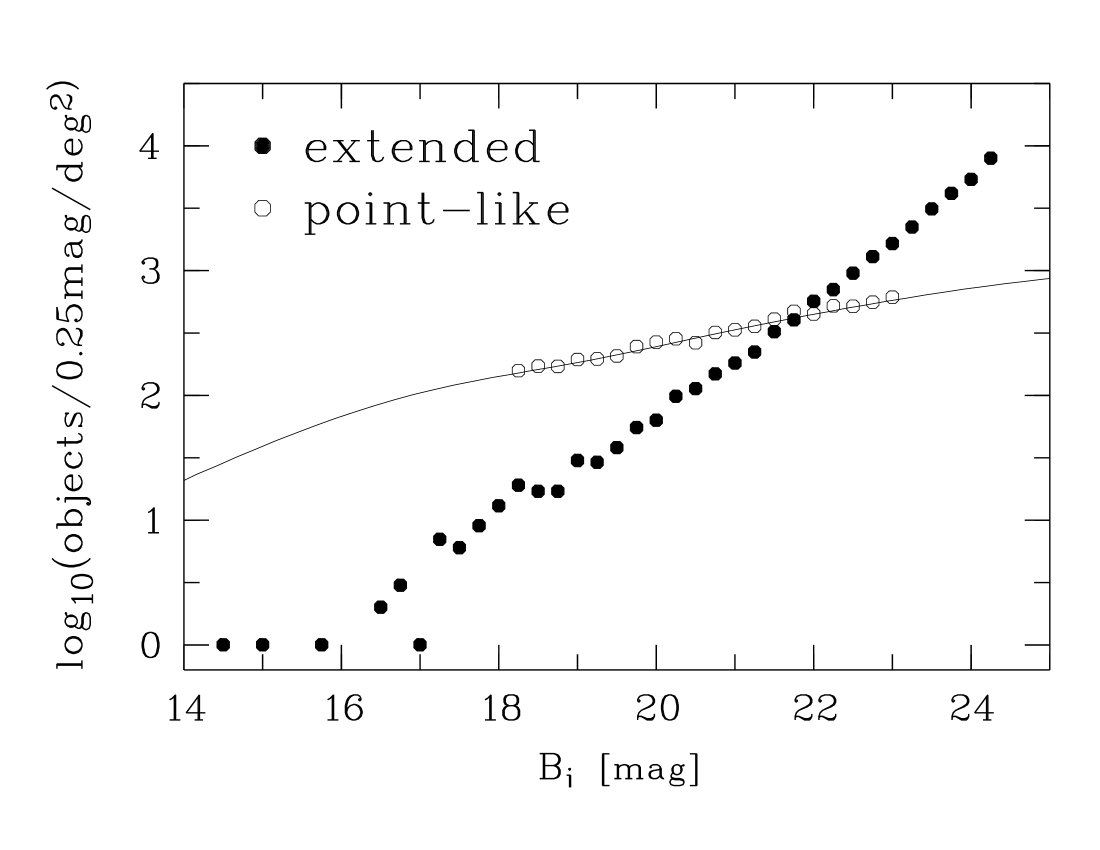
Figure 1: The number counts for extended and point-like sources in $B_{j}$. The solid line is the expected star counts according to the Bahcall-Soneira model

2.7 Astrometry

To obtain a precise absolute astrometry for the detected objects the Guide Star Catalog 1.2 (GSC) was used (Lasker et al. lasker (1990), Russel et al. russel (1990), Jenkner et al. jenkner (1990)). There are 430 GSC-stars in the area covered by our surveys, and the number of GSC-stars per exposures ranges from $1$ to $11$. All GSC-stars except the brightest one (the planetary nebula NGC 6543, $m_{V}=9.8\,\mathrm{mag}$) were taken to establish the astrometry. We identified the GSC-stars on the survey images and determined plate constants for every observing run and filter using gnomonic projection (see Eichhorn eichhorn (1974)). Using the plate constants and the position of the GSC-stars we then computed the equatorial position of every image center, and, finally, the equatorial positions of all objects found on the images.
Because of the different spacing of the exposures the position of an object in $B_{j}$ and $R$ is based on a different set of GSC-stars. The astrometry can therefore considered to be independently derived for the $B_{j}$- and the $R$-survey. We took advantage of this in order to compensate for the variable number of GSC-stars per image and to enhance the overall homogeneity of the astrometry. For every overlap between an individual $B_{j}$-frame B_k and an individual $R$-frame R_l we computed $\Delta\alpha_{kl}$ and $\Delta\delta_{kl}$, the mean offset between the $B_{j}$- and $R$-coordinates of bright stars in right ascension and declination, respectively. Then we derived the corrections $\Delta\alpha_{R_{k}}=\sum_{l}\Delta\alpha_{kl}$ and $\Delta\delta_{R_{k}}=\sum_{l}\Delta\delta_{kl}$ ($\Delta\alpha_{B_{l}}=\sum_{k}(-\Delta\alpha_{kl})$ and $\Delta\delta_{B_{l}}=\sum_{k}(-\Delta\delta_{kl})$ for B_l) and applied them to all positions in the whole frame. This procedure was iterated once to minimize the contribution of a frame with bad astrometry to its overlaps.
We estimated the accuracy of the astrometry using bright stars in the large ($\sim 1^{\prime}$) overlap regions between adjacent fields of the $R$-survey. The accuracy of the object positions was, even for the faintest sources, determined to be $<0.8^{\prime\prime}$ in each coordinate.

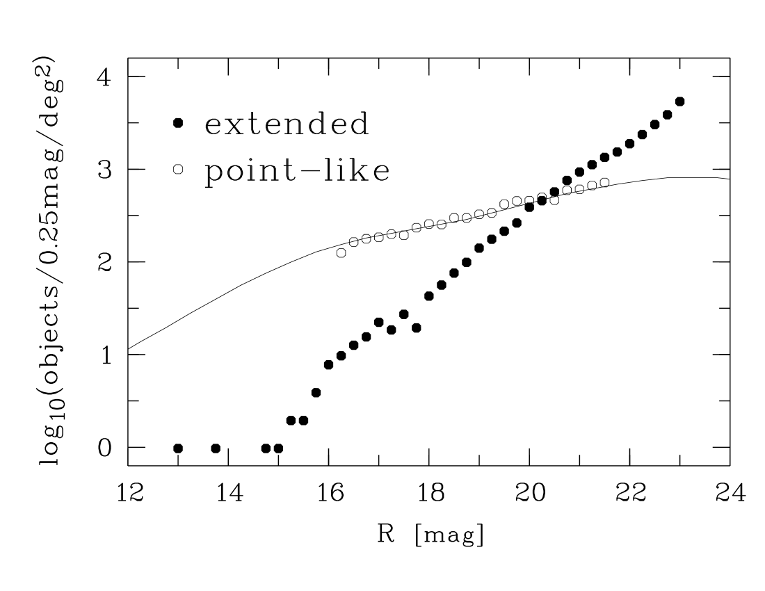
Figure 2: The number counts for extended and point-like sources in $R$. The solid line is the expected star counts according to the Bahcall-Soneira model

2.8 Removal of cosmic ray objects

Since most of the survey area is covered only by one frame, the usual approach to remove cosmics with weighting maps or masks (Nonino et al. nonino (1999), Arnouts et al. arnouts (1999)) could not be followed. Instead we identified sources caused by cosmic ray events and removed them from the object lists.
The criterion whether an object is real or just a cosmic ray hit is the concentration of the brightness distribution

$$conc=2.5*\log((Lc/9.0-ispht)/(ssbr/3.0))+mag$$ (3)

The PSF sets an upper limit in the brightness concentration for real objects. Cosmic ray hits usually have higher values of $conc$, since their shape is not determined by the PSF and a cosmic ray event usually affects only a few pixels. $Conc$ is easily derived from the FOCAS-parameters $Lc$ (core luminosity), $ispht$ (isophotal brightness) and $ssbr$ (sky-noise) together with the object brightness $mag$ (the nomenclature of the FOCAS-parameters follows Valdes valdes82 (1982)).
Looking at the $conc$-$mag$ distribution of all objects from an individual image the locus of cosmic ray objects could be identified easily and the objects could then be removed from the lists.

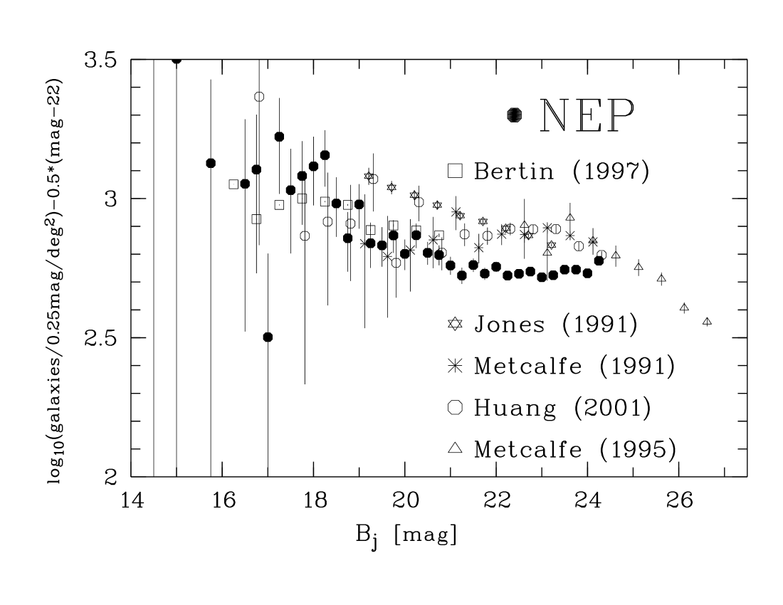
Figure 3: The galaxy counts in $B_{j}$ from the NEP compared to counts from various other surveys

3 Object counts

3.1 Extended and point-like sources in $B_{j}$ and $R$

Figs. 1 and 2 display the object counts in $B_{j}$ and $R$, respectively. In both figures the counts of point-like sources are marked with open circles, the counts for extended sources are denoted with the filled symbols. We made no attempt to correct the counts beyond the incompletentness of the individual frames. The counts were only derived from fields complete to the specific magnitude. Tables 2 and 3 give the number counts (in $objects/0.5\mathrm{mag}/\mathrm{deg}^{2}$) $B_{j}$ and $R$, respectively. The counts for extended objects are listed in column $3$ and counts for point-like objects in column $5$. The fourth column reflects pure Poissonian error of the counts for extended objects. The last column gives the area of the sub-survey complete to the specified depths. To complete the information concerning number counts in our surveys we added the corresponding data for the $K$-survey in Table 4.
The point-like sources in Figs. 1, 2 and in Tables 2-4 are only given down to the magnitude of reliable classification. The deeper counts of extended objects have been derived by subtracting the expected number of point-like objects from the counts of all objects (see Sect. 2.5 and below). No number densities can be given at the bright end of the point-like sources because the objects saturated the CCD. The solid line in Figs. 1 and 2 shows the theoretically expected stellar counts according to the Bahcall-Soneira model (Bahcall & Soneira bahcall1 (1980), Bahcall bahcall2 (1986)). To calculate the model counts in $B_{j}$ we transferred the original $V$-counts with the model $B-V$-colours and equations given by Gullixson et al. (gully (1995)). For the $R$-counts we changed the code according to Mamon & Soneira (mamon (1982)). No attempts were made to improve the fit to our data by changing the parameters of the model. This is justified by the good agreement between our counts and the model.
The Bahcall-Soneira model does not take into account the so called thick disc introduced by Gilmore & Reid (gilmore (1983)). However, the scope of the comparison done in this paper is not to test a particular model of the Galaxy. The agreement between the counts for point-like objects and the Bahcall-Soneira model is taken as confirmation of the statistical classification applied to the total counts to derive the fraction of extended objects (see chap. 2.5).

3.2 Number densities of galaxies

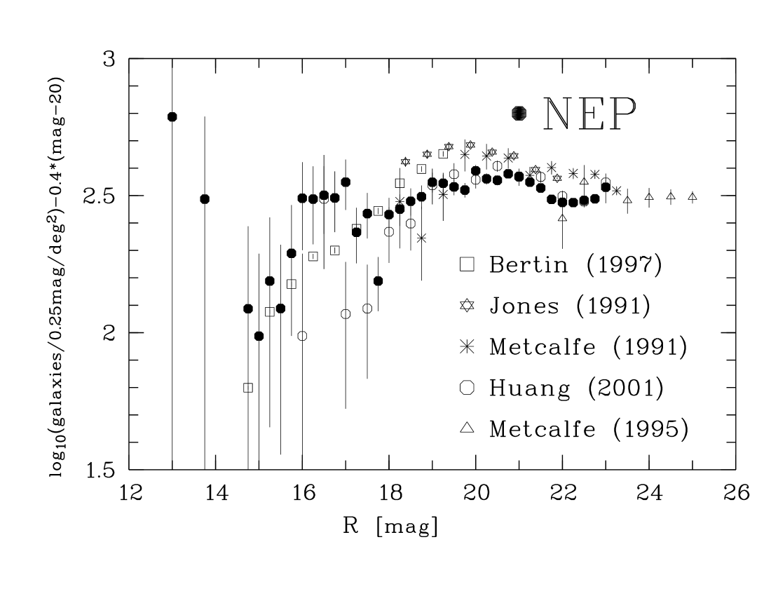
Figure 4: The galaxy counts in $R$ from the NEP compared to counts from various other surveys

In Figs. 3 and 4 we compare counts of galaxies at the NEP with published counts from other surveys in $B_{j}$ and $R$, respectively. The reference data are from Bertin & Dennefeld (bertin97 (1997)), Jones et al. (jones (1991)), Huang et al. (huang (2001)) and Metcalfe et al. (metcalfe91 (1991), metcalfe (1995)). All $B_{j}$-counts except Huang et al. (huang (2001)) were either performed in a $B_{j}$-filter or transformed to $B_{j}$ using equations given by the authors. To the Huang et al. (huang (2001)) photometry we applied the transformation $B_{j}=B-0.19\,\mathrm{mag}$, according to Bertin & Dennefeld (bertin97 (1997)) for $B-R=1.0\,\mathrm{mag}$. In the Figs. 3 and 4 the slope $0.5$ and $0.4$ is subtracted from the logarithm of the counts to expand the ordinate and to make differences between the counts clearly visible. In order to do a quantitative comparison we fitted power-laws of the form

$$N(mag)=a*10^{b*(mag-c)}$$ (4)

to the data. Tables 5 and 6 show the results of those fits. Both Tables give the literature reference and the survey area, respectively, (in deg²) in the first two columns. The next columns show the slope $b$, amplitude $a$ and the magnitude range in which the fits were done. In $B_{j}$ and $R$ the fits were done for $c=22.0\,\mathrm{mag}$ and $20.0\,\mathrm{mag}$, respectively. The faintest magnitude bins are not included in the fit. The numbers in those bins might be affected by Eddington-bias (Eddington eddi (1913)), and could influence the fits presented in Tables 5 and 6 significantly since their high values are associated with small (relative) errors.
We fitted different power-laws above and below $19.4\,\mathrm{mag}$ to the $R$-band data from the NEP, since there is a clear break in the number counts at this level. While the slope is almost $0.5$ for the bright magnitudes, it flattens by more than $0.1$ towards fainter magnitudes.
The slopes in $B_{j}$ are in good agreement with other surveys with the exception of Metcalfe et al. (metcalfe (1995)). As can be seen in Fig. 3, the change in slope at $B\sim 24$ (Arnouts et al. arnouts (1999), Williams et al. williams (1996)) flattens the slope in the deep surveys of Metcalfe et al. (metcalfe (1995)). While the slope of the NEP-counts in $B_{j}$ is comparable to the slope of other surveys to the same limiting magnitudes, the amplitude is at $a=566$ very low compared to the others, which show values around $720$.
In $R$ the NEP-counts clearly resolve the break in the slope at $19.0\,\mathrm{mag}$ leading from $0.5$ at the bright counts to $0.37$ at the faint end. As is the case in $B_{j}$ the slopes at the NEP agree well with the other surveys, but the amplitudes are lower.
The main reason for the low amplitudes in both the $B_{j}$- and the $R$-filters can be attributed to the low galactic latitude and therefore high extinction value. While typical extragalactic survey fields used e.g. in Metcalfe et al. (metcalfe (1995)) have $E_{B-V}=0.02$ the extinction at the NEP is $E_{B-V}=0.05$. This can be translated into a fading of $0.12\,\mathrm{mag}$ and $0.07\,\mathrm{mag}$ (Schmidt-Kaler schmika (1982)) of the NEP-sources with respect to sources from other surveys in $B_{j}$ and $R$, respectively. This is supported by the fact that at the longest wavelength $K$ there is no such effect (see paper I) while the difference in the amplitude is strongest in $B_{j}$, the shortest wavelength.
Assuming all of the offset is due to extinction, would lead us to shift our $B_{j}$- and $R$-counts by $\Delta B_{j}=0.2$ and $\Delta R=0.15\,\mathrm{mag}$, respectively, corresponding to an extinction of $\Delta E_{B-V}=0.05$ more than those adopted for the fields observed e.g.  by Metcalfe et al. (metcalfe (1995)). The extinction at the NEP then would have to be $E_{B-V}=0.07$, $0.02$ higher than the values from Schlegel et al. (schlegel (1998)) (see Table 1), or the extinction towards the Metcalfe et al. (metcalfe (1995)) fields would have to be negligibly small. If the extinction given by Schlegel et al. (schlegel (1998)) is taken into account, the difference between the counts at the NEP and other surveys reduces to an acceptable amount of $\sim 10\%$.

Table 5: A quantitative comparison of galaxy counts in different $B_{j}$-surveys

survey	area	slope	amplitude	range
Bertin	$140$	$0.464\pm 0.001$	$663\pm 5$	16.0-21.0
Jones	$2.1$	$0.442\pm 0.003$	$801\pm 5$	18.96-23.46
NEP	$1.0$	$0.479\pm 0.005$	$566\pm 7$	14.38-23.63
Metc.91	$0.079$	$0.491\pm 0.009$	$748\pm 27$	18.88-24.38
Huang	$0.19$	$0.473\pm 0.006$	$764\pm 18$	16.75-24.75
Metc.95	$0.005$	$0.396\pm 0.001$	$1125\pm 143$	22.37-26.87

Table 6: A quantitative comparison of galaxy counts in different $R$-surveys

survey	area	slope	amplitude	range
Bertin	$140$	$0.537\pm 0.001$	$579\pm 3$	14.5-19.5
NEPa	$1.0$	$0.480\pm 0.020$	$397\pm 30$	14.13-19.38
NEPb	$1.0$	$0.498\pm 0.044$	$424\pm 54$	17.88-19.38
Jones	$3.0$	$0.360\pm 0.002$	$448\pm 4$	18.13-22.13
NEPc	$1.0$	$0.368\pm 0.006$	$368\pm 5$	18.88-22.38
Metc.91	$0.079$	$0.370\pm 0.008$	$432\pm 21$	19.0-23.5
Huang	$0.19$	$0.357\pm 0.009$	$397\pm 14$	19.25-22.75
Metc.95	$0.006$	$0.399\pm 0.017$	$315\pm 55$	21.75-25.25

4 Galaxy colours

Changing slopes in number counts can lead to identifications of additional components contributing to the entire sample of objects, but it is impossible to constrain the nature of such additional components from number counts alone. Surveys in multiple colours provide further insight.

4.1 Matching of the $B_{j}$-, $R$- and $K$-catalogs

The colours of objects are derived by matching the independently produced catalogs in $B_{j}$, $R$ and $K$. For every entry in the $R$-catalog we searched the $B_{j}$-catalog for an object closer than $2^{\prime\prime}$ to the $R$-position. If there exists such an entry in $B_{j}$, The $R$ and the $B_{j}$ object are considered to be identical, and an entry in the $B_{j}-R$-colour catalog is made. The same procedure was applied to the $K$ and $R$ catalogs to assemble the $R-K$-colour catalog. Finally, we matched the $B_{j}$ catalog with the colour catalog in $R-K$ to get the full colour information of all objects. Since the magnitudes derived as outlined in Sect. 2.4 are “total” magnitudes, the colours were calculated as the difference between the magnitudes in each passband.
We took $2^{\prime\prime}$ as the largest distance for the identification of objects in two catalogs. At distances $>2^{\prime\prime}$ an increasing number of object pairs would enter the colour-catalogs which are just a positional coincidence by chance of two individual objects in the catalogs of each passband.

4.2 The colour-magnitude diagram in $B_{j}-R$ and $R-K$

Figs. 5 and 6 show the colour-magnitude diagrams of extended objects in $B_{j}-R$ and $R-K$, respectively. In those diagrams the morphological classification is based on the FOCAS-classifier in one filter. For $B_{j}-R$ we took the classification in $B_{j}$, and for $R-K$ the classification in $R$, since the PSF of the $K$-images is grossly undersampled (see paper I). Obviously the statistical extension of the FOCAS-classification for the number counts (see Sect 3 and paper I) could not be applied to the individual entries in Figs. 5 and 6.
Because of the misclassification at the faint end $m_{B_{j}}>23.5\,\mathrm{mag}$ (see Sect. 2.5) some actually extended objects in $B_{j}-R$ were marked as point-like sources. Those sources are not represented in Fig. 5 and the true population is underestimated there. In $R-K$ this effect starts at $R>22.5\,\mathrm{mag}$ and affects only the red faint end in Fig. 5 to a rather negligible degree.
As already argued in Sect. 2.6 sources with magnitudes down to $mag_{50}$ in $B_{j}$, $R$ and $K$ enter the colour-magnitude diagrams. The sharp cutoffs in Fig. 5 at the right (faint end) and lower right (blue-faint end) reflect the limited depth of the $B_{j}$- and $R$-exposures. Because of the colour-term in the transformation of the instrumental- to the $B_{j}$-magnitudes (see Equ. 1) the cutoff at the faint end is not parallel to the ordinate. Due to the large difference in the limiting depth of the $R$- and $K$-survey the $R$-cutoff in Fig 6 is almost unrecognizable in the sparsely populated faint red end of the colour-magnitude diagram.
Objects with unusual colours were individually inspected for errors in the reduction or matching process. Whenever a problem was detected, e.g. a different splitting of neighboring objects in the two passbands or a problem in the determination of the background near bright stars, the objects were excluded from the colour-catalogs. In $B_{j}-R$ and $R-K$ the numbers of removed objects is 30 and 20, respectively. Therefore all objects in Figs. 5 and 6, even if isolated in colour, are real objects with good photometry and colours. There are $23\,000$ and $4\,900$ points in the colour-magnitude diagrams Fig. 5 and 6, respectively.

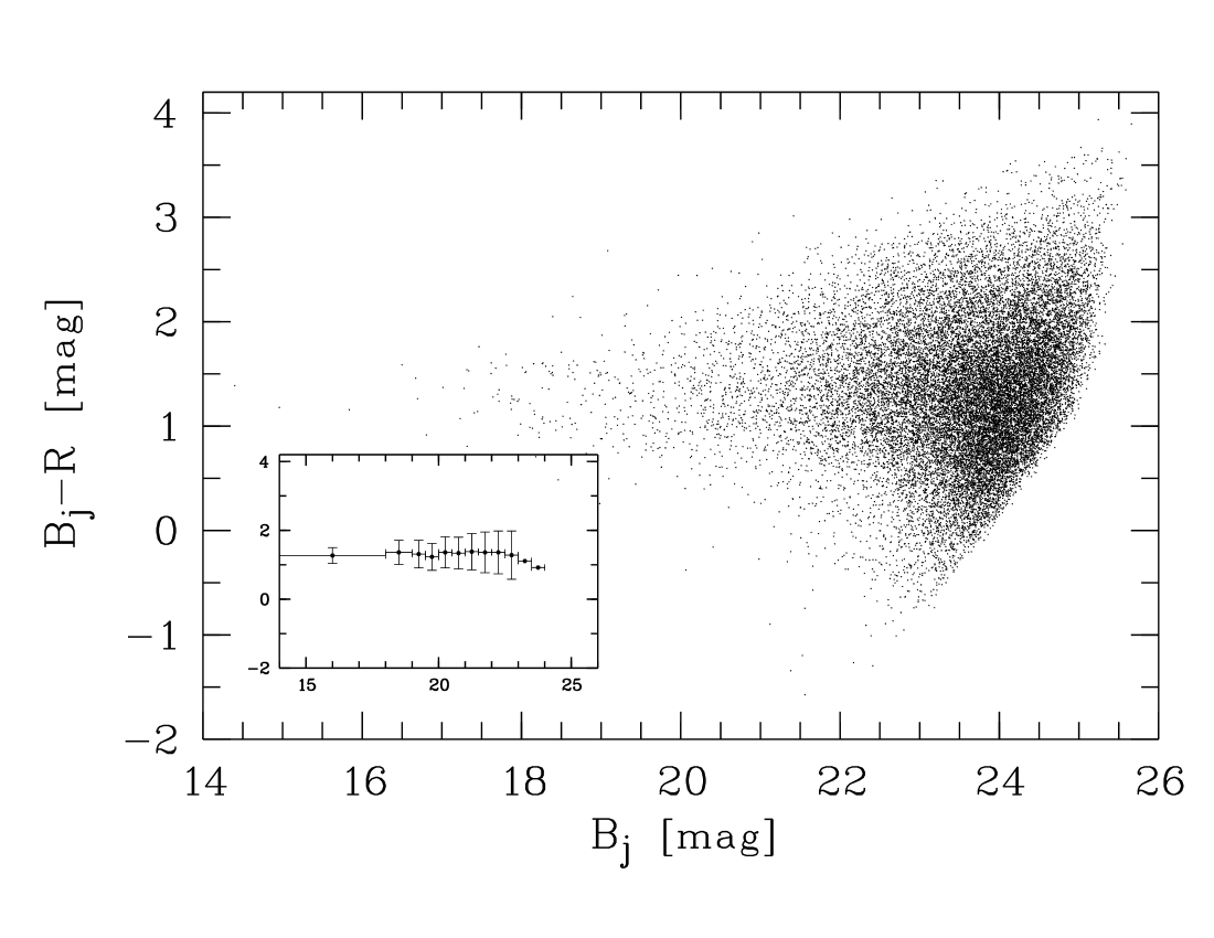
Figure 5: The colour-magnitude diagram of extended sources in $B_{j}-R$. In the inset median colours and standard deviations for magnitude bins indicated by the horizontal bars are plotted.

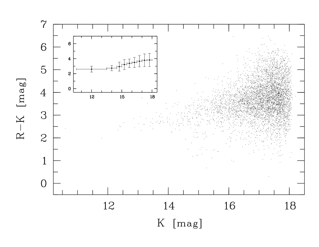
Figure 6: The colour-magnitude diagram of extended sources in $R-K$. In the inset median colours and standard deviations for magnitude bins indicated by the horizontal bars are plotted.

4.3 The two-colour diagram

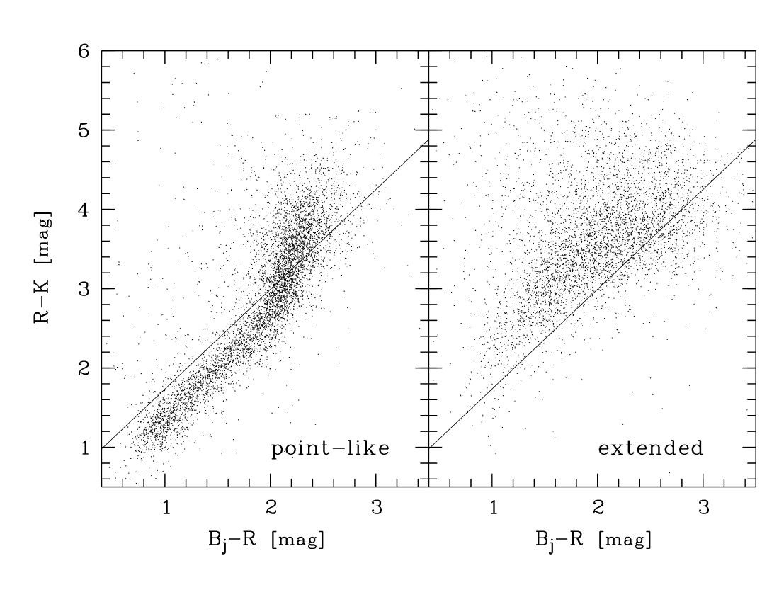
Figure 7: The two colour diagram for extended (right) and point-like (left) sources The line drawn in both panels divides point-like and extended objects in the region $B_{j}-R<1.9$.

Fig. 7 shows the two-colour diagram $B_{j}-R$ vs. $R-K$ with the point-like and extended objects in the left and right panels, respectively. As in Figs. 5 and 6 the classification into point-like (5 300 objects) and extended sources (4 200 sources) in Fig. 7 is based on the FOCAS-classification in the $R$-band. As in the colour-magnitude diagrams, only objects brighter than $mag_{50}$ in $B_{j}$, $R$, and $K$ were matched and plotted in Fig. 7.
Most of the point-like objects in the left part of Fig. 7 are concentrated along a well defined line of $\sim 0.3\,\mathrm{mag}$ width. While the blue objects are assumed to be halo stars several kpc above the galactic disc, the red objects can be identified as faint M-dwarfs within the disc, in immediate vicinity of the sun (Bahcall bahcall2 (1986), Robin & Crézé robin (1986), Baraffe et al. baraffe (1998)). The two populations are not well separated but are connected with a less densely populated regime at $B_{j}-R\sim 1.7\,\mathrm{mag}$.
Compared to point-like objects the distribution of extended objects in the two-colour diagram is much broader. Furthermore, the extended objects usually have a redder $R-K$ colour. Following Huang et al. (huang97 (1997)) this allows a separation of point-like and extended objects based on colours alone in the blue part to $B_{j}-R<1.6\,\mathrm{mag}$ at both sides of the line drawn in Fig. 7. In the red part such a colour based separation is no longer possible, since the locus of the point-like objects then lies above the separating line in the colour region populated by extended objects. Most of the 10 % contamination of unresolved galaxies in our list of point-like objects are likely to have the same distribution in the two-colour diagram as the objects classified as extended. They would hence be the dominant contribution in the sparsely populated regime with blue B_j-R and red R-K colours.

4.4 Colour trends in $B_{j}-R$ and $R-K$

In order to study the colour evolution we derived the median colour and its standard deviation in bins of apparent magnitude. The values are given in Table 7 and displayed in the insets of Figs. 5 and 6. The horizontal bars mark the widths of the bins in magnitude. For the last two bins in Fig. 5 a standard deviation could not be determined, since a significant population of blue objects are beyond the depth of the $R$-survey. In a similar way the last bin in Fig. 6 is affected by very red objects being missed in the $R$-survey. Nevertheless it is possible to put those $B_{j}$-objects without $R$-counterparts at the blue end of the colour distribution to compute the median displayed in Fig. 5.
The median $B_{j}-R$ colour of the galaxies remains constant at $\langle B_{j}-R\rangle=1.36$ from the brightest objects down to $m_{B_{j}}=22.3\,\mathrm{mag}$. Then follows a rapid evolution to bluer colours, reaching $\langle B_{j}-R\rangle=0.92$ at the faintest bin. This evolution is triggered by the onset of the population of faint blue galaxies, with $m_{B_{j}}>22.5\,\mathrm{mag}$ and $\langle B_{j}-R\rangle<0\,\mathrm{mag}$. While the full population is present down to $m_{B_{j}}>23\,\mathrm{mag}$, only its reddest part can be seen in Fig. 5 at fainter magnitudes, because the bluer ones have no counterparts in the $R$-survey.
In $R-K$ there is a steady trend to redder colours towards fainter magnitudes. The median of $\langle R-K\rangle=2.60\,\mathrm{mag}$ at the bright end changes to $\langle R-K\rangle=3.82\,\mathrm{mag}$ at $K=17.8\,\mathrm{mag}$. In the last two bins the evolution to red colours seems to level off with the median colour remaining almost constant.

Table 7: The median colours ($med_{B_{j}R,RK}$) and standard deviations ($\sigma_{B_{j}R,RK}$) in $B_{j}-R$ and $R-K$ for magnitudes slices in $B_{j}$ and $K$, respectively

$B_{j}$-range	$med_{B_{j}R}$	$\sigma_{B_{j}R}$	$K_{j}$-range	$med_{RK}$	$\sigma_{RK}$
16.0-18.0	1.27	0.23	10.5-13.5	2.60	0.39
18.0-19.0	1.36	0.35	13.5-14.5	2.74	0.35
19.0-19.5	1.31	0.40	14.5-15.0	2.94	0.60
19.5-20.0	1.23	0.39	15.0-15.5	3.22	0.67
20.0-20.5	1.36	0.45	15.5-16.0	3.38	0.57
20.5-21.0	1.34	0.46	16.0-16.5	3.50	0.66
21.0-21.5	1.38	0.53	16.5-17.0	3.66	0.75
21.5-22.0	1.36	0.59	17.0-17.5	3.79	0.85
22.0-22.5	1.36	0.62	17.5-18.0	3.82	0.87
22.5-23.0	1.28	0.70
23.0-23.5	1.11
23.5-24.0	0.92

4.5 An upper limit to $B_{j}$ dropouts

An obvious aim for wide-angle surveys is the derivation of number densities of rare classes of objects. Cosmologically important targets are highly redshifted targets which can be identified as drop-out objects when the Lyman edge is redshifted to long wavelengths, out of the bandpass of individual filters. We determine limits to the surface density of candidates for high redshifted objects. This allows constraints on the bright end of the luminosity function of highly redshifted sources. The $K$-band limits are not faint enough to include $R-K$ colour as selection criterion, and we are confined to the $B_{j}-R$ index, which does not provide a unique identification of highly redshifted sources. Nevertheless, it is interesting for deep wide-angle surveys to determine the surface density of candidate sources. All $R$-band sources above the completeness limit of our sample have a counterpart in the $B_{j}$ catalog. The only exceptions to this are a small number of faint sources close to very bright stars, where the decomposition of faint sources and halo has different efficiency in the two bands (see section 4.2). There are no true drop-outs in our sample. The amount of the decrement at the Lyman break is discussed controversially. For non-active galaxies without Lyman $\alpha$ lines of high EW, a break of about $2.6\,\mathrm{mag}_{AB}$ magnitudes has been determined (Steidel et al. steidel (1999)). In the filter-system used in our survey, the Lyman $\alpha$-break is between $B_{j}$ and $R$ for objects with $z\sim 3.8$. Thus all objects with $B_{j}-R>2.6\,\mathrm{mag}$ can be regarded as candidates for $z\geq 3.8$ galaxies. In Table 8 we give the surface density of those candidates in subsurveys with different depth in $B_{j}$. The last column of Table 8 gives the upper limit in absolute magnitude for an object with $R=R_{lim}$ at $z=3.8$. The two values refer to the cosmologies $(q_{0},\lambda_{0})=(0.5,0.0)$ and $(0.1,0.0)$; $H_{0}=50\,\mathrm{km}/\mathrm{sec}/\mathrm{Mpc}$, respectively. Out of the $9464$ point-like as well as extended sources down to $R=21.0\,\mathrm{mag}$ we detected no $B_{j}$-band dropout over the entire $1\,\mathrm{deg}^{2}$ field. The reddest objects are at $B_{j}-R\sim 3.5\,\mathrm{mag}$. According to Steidel et al. (steidel (1999)) Lyman-break colours $G-R>3.6\,\mathrm{mag}$ for redshifts $z>4.15-4.45$, depending on the extinction. Transforming this criterion to our filter set, we expect colours $B_{j}-R>3.6\,\mathrm{mag}$ for objects with $z>4.35-4.65$. Using the formulas given in Steidel et al.( steidel (1999)) we can compute from the limit in apparent $R$-magnitude an upper limit for the absolute magnitude of objects at $z\sim 4.5$. Depending on cosmology, there are no objects with $M_{AB}(1280\,\AA)<-25.0,-26.2\,\mathrm{mag}$ for $(q_{0},\lambda_{0})=(0.5,0.0),(0.1,0.0);H_{0}=50\,\mathrm{km}/\mathrm{sec}/\mathrm{Mpc}$ respectively.

Table 8: The density of high redshift candidates from the $Ly_{\alpha}$ decrement in the $B_{j}-R$-colour

$B_{j_{lim}}$	$R_{lim}$	area	$N_{cand}$	$\rho_{cand}^{\ast}$	$M_{AB}(1350\AA)$
$<24.375$	$<21.775$	$0.3$	$131$	$451$	-24.00,-25.08
$<24.125$	$<21.525$	$0.8$	$312$	$371$	-24.25,-25.33
$<23.875$	$<21.275$	$1.0$	$287$	$287$	-24.50,-25.58

• The densities are given in $N\mathrm{deg}^{-2}$.

5 Extremely red objects

5.1 The sample of EROs

Starting from the colour-magnitude diagram Fig. 6 we selected the population of extremely red objects or EROs. To give a very conservative estimate of the surface density of those objects, we applied additional selection criteria to candidates from Fig. 6. With $K<K_{compl}$ we avoid any kind of false or spurious detection in the $K$-band. Only matches with a separation less than 1 arcsecond from $K$- and $R$-band objects are accepted for EROs (as compared to $2^{\prime\prime}$ for Fig. 6). This criterion rejects matches between one object from close, but resolved, object pairs in $R$ and their combined, unresolved counterparts in $K$. Such constellations are caused by the large pixel size and resolution in $K$ and redden the objects systematically. Since the merged $K$-object has a different position with respect to both single objects in $R$, the stronger criterion concerning separation efficiently removes such mismatches. In $R$ we accepted for the EROs every object as counterpart, in contrast to Fig. 6 where only sources with $mag<mag_{50}$ were considered. While this might result in matches with non-existing sources in $R$, no false EROs are produced since the $R-K$ colour of a solid detection in $K$ can only become bluer. Finally, both authors individually checked the ERO candidates for signs of errors in detection, photometry and matching of the counterparts in $R$ and $K$. Only objects confirmed by both authors are considered as EROs. As $R$-dropouts, objects which only have a lower limit in their $R-K$-colour we considered only objects with $K<K_{compl}$. To test for errors the objects were individually checked on the $K$-images.

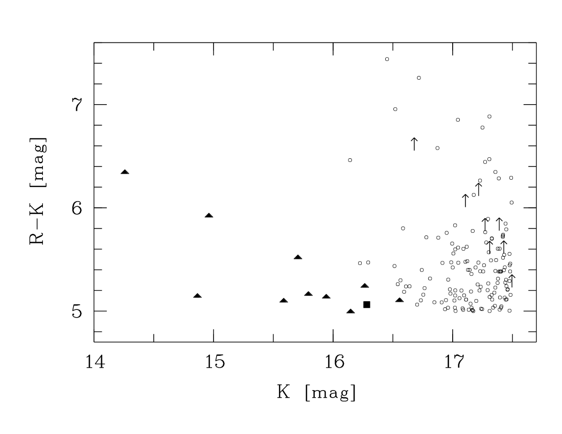
Figure 8: The colour-magnitude diagram of the EROs. Extended and point-like objects with reliable classification are marked as filled square and triangles, respectively. $R$-band dropouts are marked with their lower limit.

5.2 The surface density of EROs

Fig. 8 shows the colour-magnitude diagram of the EROs in our survey. Unfortunately the threshold for EROs in $R-K$ is not very well defined, and the values vary from $R-K>5.0$ (Cimatti et al. cim (1999)) to $R-K>6.0$ (Thompson et al. thomps (1999)). Therefore all objects with $R-K>5.0$ are included in Fig. 8. ERO objects without detection in $R$ ($R$-dropouts) are included with their lower limit in $(R-K)_{lim}$ (computed via $R_{compl}-K$) in Fig. 8. In Table 9 we give the surface density of the our EROs for different limits in $K$-magnitude as well as colour $R-K$. Only EROs in sub-surveys complete down to the $K$-limit specified in the first column of Table 9 are taken to compute the surface densities. The area of those sub-surveys is given in the last column of Table 9 (see also paper I). The $R$-dropouts were taken with their respective $(R-K)_{lim}$ to compute the surface densities in Table 9. The number of $R$-dropouts is given in Table 9 within parentheses.
Only $11$ EROs out of the $146$ from Fig. 8 are bright enough to allow a reliable morphological classification in $R$. While the only extended object is marked with a filled square, the point-like sources are given as filled triangles.
The two main contributors to our EROs-population are late type stars and galaxies at high redshift ($z>0.8$). As the available information on morphology suggests, the bright end is dominated by stellar objects. According to Leggett (leggett (1992)) a colour $R-K>5.0\,\mathrm{mag}$ is expected for stellar types M6 and later. With typical absolute magnitudes of $M_{K}=9.5\,\mathrm{mag}$ and $M_{K}=11.5\,\mathrm{mag}$ for M6-dwarfs and L-dwarfs, respectively (see Leggett leggett (1992) and Reid reid (1999)) and we detect these objects out to a distance of $400\,\mathrm{pc}$ and $160\,\mathrm{pc}$.
The surface density of extragalactic EROs at the depth of our survey is completely unknown. Thompson et al. (thomps (1999)) give a surface density of $0.04\,\mathrm{arcmin}^{-2}$ down to $K\leq 19.0\,\mathrm{mag}$. This is more than $5$ times higher than our value at $R-K>6.0$ for the total population at our limit $K\leq 17.5\,\mathrm{mag}$. The high surface density of $0.7\,\mathrm{arcmin}^{-2}$ as given by Eisenhardt et al. (eisen (1999)) in their sample down to $K\leq 20.1\,\mathrm{mag}$ gives clues to a fast decline of the density towards brighter magnitudes. Therefore only a few out of the $16$ objects in the reddest and deepest interval of Table 9 might be of extragalactic origin. Deeper studies of the red population would require data with both better spatial resolution and wavelength coverage.

Table 9: The density of EROs-object as a function of limits in $K$-magnitude and $R-K$ colour.

mag	$\rho_{R-K>5.0}^{\ast}$	$\rho_{R-K>5.5}^{\ast}$	$\rho_{R-K>6.0}^{\ast}$	area [deg]2
$K<15.0$	$0.09$	$0.06$	$0.03$	$0.93$
$K<16.0$	$0.21$	$0.09$	$0.03$	$0.93$
$K<17.0$	$1.43$  $(1)$	$0.43$  $(1)$	$0.21$  $(1)$	$0.91$
$K<17.5$	$5.46$  $(7)$	$1.91$  $(4)$	$0.91$  $(3)$	$0.61$

• The densities are given in $10^{-2}\mathrm{arcmin}^{-2}$.

6 Modeling of the galaxy colour-distributions in $B_{j}-R$ and $R-K$

The colour trends seen in the colour magnitude diagrams in Sect. 4.2 are caused by a combination of different stellar populations sampled in galaxies of higher redshift (and therefore observed at fainter magnitudes) and colour corrections introduced through cosmological effects, the so called k-corrections. A method to compute colour distributions taking into account those effects involves the so called pure luminosity evolution models (Gardner gardner98 (1998), Pozzetti et al. pozzetti (1996)). The data in our surveys give the unique opportunity to compare two observed colour distributions with those models. Our large number of sources allows us to reject models which do not reproduce the observed distribution with a high significance. Note, that in $R-K$ the comparison is not affected by an incomplete coverage of red $K$-objects in $R$.

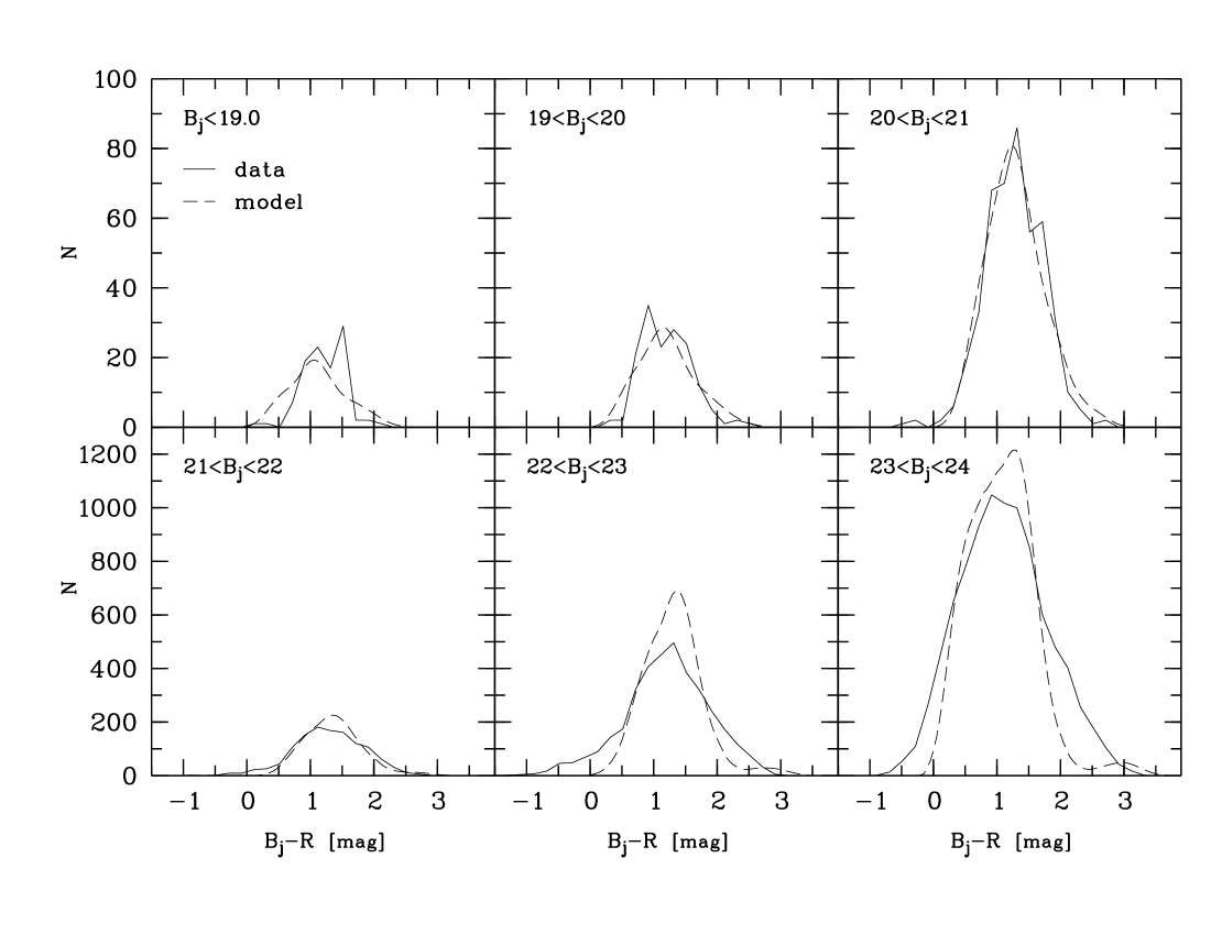
Figure 9: The colour-distribution of galaxies in $B_{j}-R$ (solid line) in comparison with the distribution of the model described in the text (dashed line).

6.1 Modeled colour distributions

This modeling is based on theoretical spectral energy distributions (SEDs) computed with evolutionary synthesis techniques by Bruzual & Charlot (bruzual (1993)). To derive the colour-distributions from the input parameters SEDs, luminosity function, cosmology and SED-mix (or type mix) we used the program ncmod developed by Gardner (gardner98 (1998)). The basic characteristics of the SEDs used in terms of corresponding galaxy type, metallicity, star formation rate, and epoch of first stars $z_{form}$ are given in Tab. 10. The last column indicates whether passive evolution of the galaxy luminosity is taken into account or not. In all models presented here the cosmological parameters $H_{0}=50\,\mathrm{km}/\mathrm{sec}/\mathrm{Mpc}$, $q_{0}=0.02$ and $\lambda_{0}=0.0$ have been used. Likewise, all models consider internal absorption by dust according to Wang (wang (1991)).
For the theoretical distribution of $B_{j}-R$ we assume the $B_{j}$-based luminosity function of Loveday et al. (loveday (1992)) and a type mix of 0% E1, 10% E2, 10% Sa, 15% Sbc, 45% Scd, and 20% Irr.
In $R-K$ we show two models using the $K$-luminosity function from Gardner et al. (gardner97 (1997)). The type mix is 16% E1, 16% E2, 28% Sa, 29% Sbc, 5% Scd, and 6% Irr for model 1, and 25% E1, 25% E2, 36% Sa, 10% Sbc, 3% Scd, and 1% Irr for model 2.

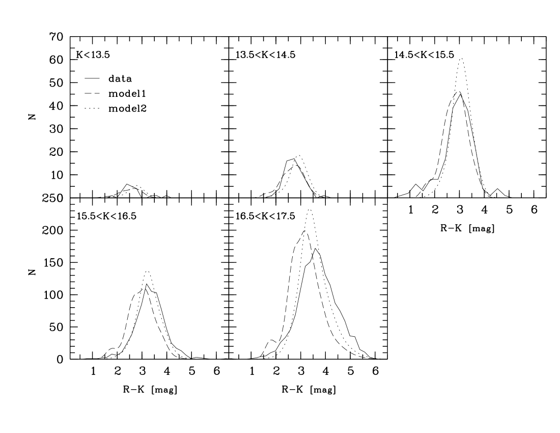
Figure 10: The colour-distribution of galaxies in $R-K$ (solid line) in comparison with the distribution of the models described in the text (model1: dashed line, model2: dotted line).

Table 10: Description of the SEDs used to model the galaxy colours.

type	metalicity	star formation rate	$z_{\rm form}$	evolution
E1	$2.5\times$solar	exp., $\tau=1\,$Gyr	$15$	y
E2	$1.0\times$solar	exp., $\tau=1\,$Gyr	$15$	y
Sa	$1.0\times$solar	exp., $\tau=4\,$Gyr	$15$	y
Sbc	$0.4\times$solar	exp., $\tau=7\,$Gyr	$15$	y
Scd	$0.2\times$solar	const.	$15$	y
Irr	$0.2\times$solar	const.	$1$	n

6.2 Comparison of modeled and observed colour distribution

Figs. 9 and 10 show the comparison between the models and the observed colour distribution in $B_{j}-R$ and $R-K$. The data are shown in solid, the models in the dashed and dotted lines. While the observed distributions have been corrected for galactic absorption by $\Delta(R-K)=-0.10\,\mathrm{mag}$ and $\Delta(B_{j}-R)=-0.08\,\mathrm{mag}$ (see Tab. 1 and Schmidt-Kaler schmika (1982)), the theoretical distributions in Figs. 9 and 10 were folded with a Gaussian of $0.2\,\mathrm{mag}$ FWHM in order to mimic photometric errors.
In the comparison between models and data we had to treat the colour distributions in $B_{j}-R$ and $R-K$ separately since none of the models reproduces the colour distribution in $B_{j}-R$ and $R-K$ simultaneously for a single luminosity function and type mix.
Fig. 9 compares the $B_{j}-R$-colour distribution of galaxies in bins of different apparent magnitude $B_{j}$ to the best fitting theoretical colour distribution (computed as described in Sect. 6.1). The agreement of the models with the data is very good throughout the magnitude range covered. There are small deviations only in the last two panels ($B_{j}>22\,\mathrm{mag}$). In the $B_{j}=22.5\,\mathrm{mag}$ bin an agreement could easily be reached using a broader Gaussian filter, which is justified by the larger photometric errors at the faint end. The last panel at $B_{j}=23.5\,\mathrm{mag}$ is seriously affected by incompleteness in both $B_{j}$ and $R$, which affects the observed colour distribution.
Fig. 10 shows the $R-K$-colour distribution of galaxies together with the two models outlined in Sect. 6.1. Neither model 1 nor model 2 is able to reproduce the observed galaxy colours in $R-K$ over the complete range in apparent magnitude in $K$. This is caused by the strong evolution of the whole population to redder colours as already demonstrated in Sect. 4.2. While model 1 agrees with the observed distribution at the bright end, but is too blue at the faint end, model 2 agrees at the faint end but is too blue at bright $K$-magnitudes. None of the models can follow the trend of the observed distributions which become redder by $\sim 1\,\mathrm{mag}$ in the range $K=13.5-17.5\,\mathrm{mag}$.

7 Summary

We have performed a medium deep survey in the filters $B_{j}$, $R$ and $K$ with completeness limits $24.25$, $23.0$ and $17.5\,\mathrm{mag}$, respectively in the central square degree around the Northern Ecliptic Pole.
We have derived the object number counts for point-like and extended sources in $B_{j}$ and $R$ and compared our results for the extended sources to other galaxy number counts found in the literature by fitting a power law to the data. In both filters we confirm the slope in dlogN/dm found in other, smaller surveys with values around $0.48$ and $0.37$ in $B_{j}$ and $R$, respectively. Differences in the absolute numbers, represented by the amplitude of the power law fits, can largely be attributed to galactic extinction and the limited accuracy of reddening corrections.
We have determined the colour distribution of galaxies in $B_{j}-R$ and $R-K$ in a large range of 10 magnitudes down to $B_{j}=24.0$ and $K=18.0\,\mathrm{mag}$, respectively. In $B_{j}-R$ the median colour remains constant to $B_{j}=22.3\,\mathrm{mag}$ and become bluer to fainter levels. This trend to bluer colours marks the onset of the so called ”faint blue galaxies” (Ellis ellis (1997)). In R-K the galaxies become redder from a medium colour $R-K=2.6$ at $K=12\,\mathrm{mag}$ to $R-K=3.8$ at $K=17.8\,\mathrm{mag}$.
For the filter system used in our survey we have given lower limits for the expected colours (in $B_{j}-R$) of Lyman-break galaxies at $z\sim 3.8$. We derive the surface densities for candidates found in our survey. From the reddest objects in $B_{j}-R$ found in our survey we have derived the lower limit for Lyman-break galaxies at $z>4$ to $M_{AB}(12280\,\AA)>-25.0\,\mathrm{mag}$ (for $q_{0}$, $\lambda_{0}$, $h_{0}=0.5,0.0,0.5$).
We have determined the surface density of red objects ($R-K>5.0\,mag$) down to $K=17.5\,\mathrm{mag}$ on the basis of our large field of view ($0.9\,\mathrm{deg}^{2}$). Since we are unable to determine the morphology of most of the objects, the surface densities include late type stars (M6 and later) as well as the extragalactic EROs. At the bright end (K$<16.5\,\mathrm{mag}$), which has reliable morphological classification, point-like objects dominate the sample. While the surface density of objects with $R-K>6$ declines by a factor of twenty from $20.0\,\mathrm{mag}$ to $19.0\,\mathrm{mag}$ (Eisenhardt et al. eisen (1999), Thompson et al. thomps (1999), Daddi et al. daddi (2000)), we find the surface density at $17.5\,\mathrm{mag}$ to be reduced only by an additional factor of four. This comparison shows that either the steep decline in density from $K=20$ to $19\,\mathrm{mag}$ levels off to $K=17.5$ or that a large fraction of our extremely red objects are stars.
We have compared the colour distribution of galaxies in $B_{j}-R$ and $R-K$ with theoretical colours based on spectral evolution synthesis. We have shown that it is not possible to find parameters (e.g. luminosity function and galaxy type mix) such that both colour distributions are reproduced simultaneously. While a type mix dominated by late type galaxies reproduces the optical colour $B_{j}-R$, the strong trend to redder colours in $R-K$ with increasing magnitudes can not be reproduced by models. A model which fits the data at $K=17\,\mathrm{mag}$ is too red at $K=14\,\mathrm{mag}$, a model which fits at the bright end is too blue at the faint end.