Computer simulations of interferometric imaging with the
VLT interferometer and its AMBER instrument

Abstract

We present computer simulations of interferometric imaging with the Very Large Telescope Interferometer (VLTI) of the European Southern Observatory (ESO) and the Astronomical MultiBEam Recombiner (AMBER) phase-closure instrument. These simulations include both the astrophysical modelling of a stellar object by radiative transfer calculations and the simulation of light propagation from the object to the detector (through atmosphere, telescopes, and the AMBER instrument), simulation of photon noise and detector read-out noise, and finally data processing of the interferograms. The results show the dependence of the visibility error bars on the following observational parameters: different seeing during the observation of object and reference star (Fried parameters $r_{0,{\rm object}}$ and $r_{0,{\rm ref.}}$ ranging between 0.9 m and 1.2 m), different residual tip-tilt error ($\delta_{\rm tt,object}$ and $\delta_{\rm tt,ref.}$ ranging between 0.1% and 20% of the Airy disk diameter), and object brightness ($K_{\rm object}$=0.7 mag to 10.2 mag, $K_{\rm ref.}$=0.7 mag). Exemplarily, we focus on stars in late stages of stellar evolution and study one of its key objects, the dusty supergiant IRC +10 420 that is rapidly evolving on human timescales. We show computer simulations of VLT interferometry (visibility and phase closure measurements) of IRC +10 420 with two and three Auxiliary Telescopes (ATs; AMBER wide-field mode, i.e. without fiber optics spatial filters) and discuss whether the visibility accuracy is sufficient to distinguish between different theoretical model predictions.

Keywords: astronomy, infrared, interferometry, radiative transfer, simulations, telescopes

1 INTRODUCTION

The Very Large Telescope Interferometer[1] (VLTI) of the European Southern Observatory (ESO) with its four 8.2 m unit telescopes (UTs) and three 1.8 m auxiliary telescopes (ATs) will certainly establish a new era of optical and infrared interferometric imaging within the next few years. With a maximum baseline of up to more than 200 m, the VLTI will allow the study of astrophysical key objects with unprecendented resolution opening up new vistas to a better understanding of their physics.

The near-infrared focal plane instrument of the VLTI, the Astronomical MultiBEam Recombiner[2, 3] (AMBER), will operate between 1 and 2.5 $\mu$m and for up to three beams allowing the measurement of closure phases. In a second stage its wavelength coverage is planned to be extended to 0.6 $\mu$m. Objects as faint as $K=20$ mag are expected to be observable with AMBER when a bright reference star is available, and as faint as $K=14$ mag otherwise.

Among the astrophysical key issues[4] are, for instance, young stellar objects, active galactic nuclei and stars in late stages of stellar evolution. The simulation of interferometric imaging of a stellar object consists in principle of two components:
(i) the calculation of an astrophysical model of the object, typically based on radiative transfer calculations predicting, e.g., its intensity distribution. To obtain a robust and non-ambiguous model, it is of particular importance to take diverse observational constraints into account, for instance the spectral energy distribution and visibilities.
(ii) the determination of the interferometer’s response to this intensity signal, i.e. the simulation of light propagation in the atmosphere and the interferometer.
Often, only one of the above parts is considered in full detail. The aim of this study is to combine both efforts and to present a computer simulation of the VLTI performance for observations of one object class, the dusty supergiants. For this purpose, we calculated a detailed radiative transfer model for one of its most outstanding representatives, the supergiant IRC +10 420, and carried out computer simulations of VLTI visibility measurements. The goal is to estimate how accurate visibilities can be measured with the VLTI in this particular but not untypical case, to discuss if the accuracy is sufficient to distinguish between different theoretical model predictions and to study on what the accuracy is dependent.

2 The supergiant IRC +10 420: Evolution on human timescales

The star IRC +10 420 (= V 1302 Aql) is an outstanding object for the study of stellar evolution. Its spectral type changed from F8 I${}_{\rm a}^{+}$ in 1973[5] to mid-A today[6, 7] corresponding to an increase of its effective temperature of 1000-2000 K within only 25 yr. It is heavily obscured by circumstellar dust due to strong mass loss with rates typically of the order of several $10^{-4}$ M_⊙/yr (M_⊙: solar mass) [8, 6]. IRC +10 420 is believed to be a massive luminous star of initially $\sim 20$ to 40 M_⊙ currently being observed in its rapid transition from the red supergiant stage to the Wolf-Rayet ddphase[9, 10, 11, 6, 7]. Wolf-Rayet stars, in turn, finally evolve into a supernova explosion. IRC +10 420 is the only object observed until now in its transition phase to the Wolf-Rayet stage.

Several infrared speckle and coronographic observations [13, 14, 15, 16, 17] were conducted to study the dust shell of IRC +10 420. The most recent study of Blöcker et al. [18] reports the first diffraction-limited 73 mas (mas: milli-arcsecond) bispectrum speckle interferometry of IRC +10 420 and presents the first radiative transfer calculations that model both the spectral energy distribution and the visibility of this key object. We will briefly describe the main results and conclusions of this study which will serve as astrophysical input for the VLTI computer simulations presented in the next section.

Figure 1: SED (top) and 2.11 $\mu$m visibility (middle) for superwind models with amplitudes $S$ (=factors of density enhancement) at $Y=r_{\rm sw}/r_{1}=4.5$, as well as normalized intensity vs. angular displacement $\vartheta$ (bottom) for the best model with $Y=r_{\rm sw}/r_{1}=4.5$ and $S=40$. In the bottom panel the (unresolved) central peak belongs to the central star. The inner hot rim of the circumstellar shell has a radius of 35 mas, and a cool component is located at 155 mas. Model parameters are: black body, $T_{\rm eff}=7000$ K, $T_{1}=1000$ K, $\tau_{0.55\mu{\rm m}}=7.0$, silicate dust grains[27], standard grain size distribution[26] with $a_{\rm max}=0.45\,\mu$m, outer dust-shell boundary=$10^{4}R_{\ast}$ ($R_{\ast}$: stellar radius), The inner shell region ($Y\leq 4.5$) obeys a $1/r^{2}$ density distribution, the outer shell region a $1/r^{1.7}$ density distribution. The symbols refer to the observations (see text) corrected for interstellar extinction of $A_{V}=5{\rm mag}$. [from Ref. 18]

Fig. 1 shows the SED[6, 11, 23, 24] and the reconstructed 2.11 $\mu$m visibility function[18] of IRC +10 420. The visibility 0.6 at frequencies $>4$ cycles/arcsec indicates, for instance, that the stellar contribution to the total flux is $\sim$ 60% and the dust shell contribution is $\sim$ 40%.

An extensive grid of radiative transfer models was calculated for the dust shell of IRC +10 420 assuming spherical symmetry and considering black bodies and model atmospheres as central sources of radiation, different silicates, grain-size and density distributions, various dust temperatures at the shell’s inner boundary (determining the radius of the shell’s inner boundary) and optical depths. We refer to Blöcker et al. [18] for a full description of the model grid. It turned out that the observed dust-shell properties cannot be matched by single-shell models but require multiple components with different density distributions. The best model was found for a dust shell with a dust temperature of $T_{1}=1000$ K at its inner radius of $r_{1}=69\,R_{\ast}$ ($R_{\ast}$: stellar radius). At a distance of $r_{\rm sw}=308\,R_{\ast}$ ($Y=r_{\rm sw}/r_{1}=4.5$) the density was enhanced by a factor of $S=40$ and its slope within the shell changed from $1/r^{2}$ to $1/r^{1.7}$. The corresponding fits for SED and 2.11 $\mu$m visibility are shown in Fig. 1. The shell’s model intensity distribution is shown in Fig. 1 and was found to be ring-like due to a limb-brightened dust-condensation zone. The ring diameter is equal to the inner diameter of the hot shell ($\sim 69$ mas), and the diameter of the central star amounts to $\sim 1$ mas.

This two-component model can be interpreted in terms of a termination of an enhanced mass-loss phase roughly 90 yr ago. The assumption that IRC +10 420 had passed through a superwind phase in its recent history is in line with its evolutionary status of an object in transition from the Red-Supergiant to the Wolf-Rayet phase.

3 Interferometry with the VLTI and the AMBER instrument

In the previous section, the spatial intensity profile of the dusty supergiant IRC +10 420 (see Fig. 1) was derived by means of radiative transfer models and their comparison with photometric and interferometric observations. This $2.11\,\mu$m intensity profile will serve as object intensity profile in the simulation of monochromatic VLTI observations. The next steps are the simulation of light propagation from the object to the detector (through atmosphere, telescopes, and the AMBER wide-field mode instrument), simulation of photon noise and detector read-out noise, and finally data processing of the interferograms.

3.1 Computer simulation of interferometric imaging

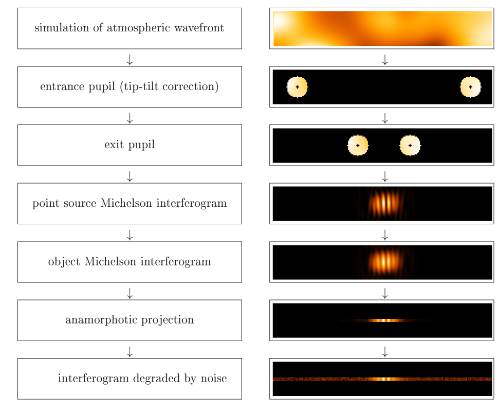
Figure 2: Flow chart of the simulation of VLTI AMBER interferograms (wide-field mode, i.e. without fiber optics spatial filtering).

Fig. 2 shows a flow chart of our simulation of interferometric imaging with the VLTI (ATs, or UTs with adaptive optics) and the AMBER camera in the wide-field mode (i.e. without fiber optics spatial filtering). The total number of detectable photons $N_{\rm tot}$ is given by the object brightness, the wavelength and band-width, the collecting area of the telescope, the total transmission of the optics, and the quantum efficiency of the detector[28]. Since we assume that the observations are carried out with a spectral resolution of $R=\lambda/\Delta\lambda=70$, the number of photons available in one spectral channel for observations in the $K$-band is given by $N_{\rm channel}=N_{K,{\rm tot}}\cdot R_{K}/R$, with $R_{K}=2.2\,\mu{\rm m}/0.4\,\mu{\rm m}=5.5$ being the spectral resolution of the $K$-band (i.e. $R/R_{K}\sim 13$ is the number of spectral channels within the $K$-band; $N_{K,{\rm tot}}$ is the total number of $K$-band photons). The simulations described below refer to observations in one spectral channel (see also Table 1). The signal-to-noise ratio of the reconstruction can be increased by averaging the reconstructions of all $R/R_{K}$ channels.

Table 1: Parameters of VLTI-AT/AMBER simulations: Wavelength, object brightness, optical throughput (=throughput of VLTI-AT + AMBER in the wide-field mode, AT mirror size: 1.8 m), read-out noise and quantum efficiency of the detector, exposure time, and photon number $N_{\rm channel}$ per frame and per one spectral channel for the lowest spectral resolution of AMBER of $R=\lambda/\Delta\lambda=70$ (instrumental AMBER characteristics taken from Malbet et al.[31])

wavelength	$K$ brightness	opt. throughput	read-out noise	quant. efficiency	exposure	photon number $N_{\rm channel}$
$2.11\,\mu$m	$0.7-10.2$ mag	0.108	15 e-	0.6	50 ms	$4.42\cdot 10^{6}-7.00\cdot 10^{2}$

In a first step, an array of Gaussian distributed random numbers is generated and convolved with the correlation function of the atmospheric refraction index variations (see Roddier[29]) in order to generate wavefronts degraded by atmospheric turbulence. The typical size of the atmospheric turbulence cells is given by the Fried parameter $r_{0}$. After the simulation of the entrance pupil, the next step incorporates the tip-tilt correction of the wavefront over each subpupil, but we allow for a residual tip-tilt error $\delta_{\rm tt}$. In the next step a typical Michelson output pupil is simulated by shifting both subpupils from the entrance pupil position, with a subpupil separation equal to the baseline, to the output pupil position where both subpupils are only separated by $\sim$ one subpupil diameter (pupil reconfiguration). The output pupil is chosen such that (i) in the optical transfer function the off-axis peaks are separated from the central peak, and (ii) the interferograms are sampled with the smallest number of pixels to assure the lowest influence of detector noise. The following step includes light propagation through the beam combiner lens to the focal plane. The squared modulus of the Fourier transform of the complex amplitude in front of the beam combiner lens yields the intensity distribution of a Michelson interferogram of a point source. In the next step the required object intensity distribution is simulated (given here by the intensity distribution of IRC +10 420) to obtain the Michelson interferogram of the object: The Fourier transformation of the object intensity distribution, calculated at those spatial frequencies covered by the the simulated interferometer baseline vector, is multiplied with the off-axis peaks of the transfer function of the generated Michelson interferogram[30]. Finally, Poisson photon-noise and detector read-out noise is injected to the interferograms. The noise level depends, among other parameters, on the number of detectable photons, the total optical throughput of the interferometer (VLTI + AMBER in the wide-field mode) and the quantum efficiency of the detector. Details[31] of the simulation parameters specific to VLTI-AT/AMBER, as optical throughput, detector read-out noise and quantum efficiency, are given in Table 1.

3.2 Computer simulations of visibility measurements

We performed simulations of IRC +10 420 visibility observations in the VLTI-AT/AMBER wide-field mode and studied the influence of various observational parameters on the visibility accuracy. Visibility error bars were obtained for the following observational parameters:

1. different seeing during the observation of object and reference star (Fried parameters $r_{0,{\rm object}}$ and $r_{0,{\rm ref.}}$ ranging between 0.9 m and 1.2 m),

2. different residual tip-tilt error ($\delta_{\rm tt,object}$ and $\delta_{\rm tt,ref.}$ ranging between 0.1% and 20% of the Airy disk diameter),

3. different object brightness ($K_{\rm object}$=0.7 mag to 10.2 mag, $K_{\rm ref.}$=0.7 mag).

All computer experiments are based on 2400 interferograms of the $S=40$ intensity profile (see Fig. 1) of IRC +10 420 and refer to observations in one of the $R/R_{K}\sim 13$ spectral channels. The error bars correspond to the reduction of six statistically independent data sets and refer to the standard deviation $\sigma$. The dependence of the error bar on the number of data sets has been verified (see below). In the computer experiments (1) and (2) mentioned above, object and reference star were assumed to have the same brightness. We chose $K$=0.7 mag (see Table 1) in order to minimize brightness effects. Experiment (3) simulates IRC +10 420 itself ($K$=3.5 mag) and fainter objects, assuming object and reference star to have the same seeing and residual tip-tilt error ($r_{0,{\rm object}}$=$r_{0,{\rm ref}}$=0.9 m; $\delta_{\rm tt,object}$=$\delta_{\rm tt,ref}$=0.1%). These simulations supersede the corresponding results of a first exploratory study [32] due to improved numerics and a broader statistical basis.

The first computer experiment (different seeing conditions) consists of the simulations A to F (see top panel of Fig. 3). Simulation A represents the case of typical seeing conditions ($r_{0,{\rm object}}$=0.9 m, $r_{0,{\rm ref.}}$=0.9 m) and an almost perfect tip-tilt correction (residual tip-tilt error $\delta_{\rm tt}=0.1$%). It will serve as a reference for the following simulations. The brightness of object and reference star was chosen to be $K$=0.7 mag. The visibility error $\sigma_{V}$ amounts only to $\pm 0.0067$. The remaining statistical uncertainty due to the limited number of data sets has been checked by a test calculation taking into account twice as many statistically independent data sets, i.e. 12 data sets instead of 6. The visibility error changed by 24% from $\pm 0.0067$ to $\pm 0.0051$. However, the general dependencies of the visibility accuracy on observational parameters (seeing, residual tip-tilt error, brightness) are only scarcely affected.

If one considers a better seeing for both object and reference star (A-C), $\sigma_{V}$ decreases in almost linear proportion with increasing diameter of the atmospheric turbulence cells (Fig 3). However, improved but different seeing conditions (D-F) lead to larger visibility errors. This emphasizes that equal seeing conditions for object and reference star are more crucial than excellent seeing conditions of, e.g., the object only in order to obtain accurate visibilities.

The second set of simulations (A, G-J) illustrates the influence of a larger residual object tip-tilt error (see middle panel of Fig. 3). Increasing $\delta_{\rm tt}$ from 0.1% to 20% for both object and reference star increases the visibility error from 0.0067 to 0.0084 (A,F,G). Like in the simulations of different seeing conditions, it is essential to have the same tip-tilt error for both object and reference star in order to achieve high accuracy. Differences in $\delta_{\rm tt}$ enhance the visibility error (H,I).

Finally, in the third experiment of this series an IRC +10 420-like intensity distribution is assumed but much much fainter (i.e. fainter than $K$=3.5 mag) objects are considered (see bottom panel of Fig. 3, simulations A, K-N). The visibility error stays almost constant up to an $K$ magnitude of 7 mag. If the simulated object $K$-magnitude is 9.2 mag, the visibility error has increased by a factor of $\sim 2$, i.e. to $\sigma_{V}=0.0156$, but is still acceptable although the photon number decreased to $N_{\rm channel}=1.76\cdot 10^{3}$ (i.e. by a factor of 2500, see Table 1). Fig. 3 demonstrates that for even fainter objects noise becomes more and more important leading to an steep increase of the visibility error. However, the signal-to-noise ratio can be improved ($\sim\sqrt{R/R_{K}}\sim 3.6$) if the visibility measurements of all $R/R_{K}$ spectral channels within the $K$-band are averaged.

		$r_{0}$ [m]	$\delta_{\rm tt}[\%]$	$K$ [mag]	$\sigma_{V}$
	obj.	0.9	0.1	0.7
A	ref.	0.9	0.1	0.7	0.0067
	obj.	1.1	0.1	0.7
B	ref.	1.1	0.1	0.7	0.0047
	obj.	1.2	0.1	0.7
C	ref.	1.2	0.1	0.7	0.0036
	obj.	1.0	0.1	0.7
D	ref.	0.9	0.1	0.7	0.0214
	obj.	1.1	0.1	0.7
E	ref.	0.9	0.1	0.7	0.0376
	obj.	1.2	0.1	0.7
F	ref.	0.9	0.1	0.7	0.0551

		$r_{0}$ [m]	$\delta_{\rm tt}[\%]$	$K$ [mag]	$\sigma_{V}$
	obj.	0.9	0.1	0.7
A	ref.	0.9	0.1	0.7	0.0067
	obj.	0.9	10	0.7
G	ref.	0.9	10	0.7	0.0072
	obj.	0.9	20	0.7
H	ref.	0.9	20	0.7	0.0084
	obj.	0.9	15	0.7
I	ref.	0.9	10	0.7	0.0080
	obj.	0.9	20	0.7
J	ref.	0.9	10	0.7	0.0107

		$r_{0}$ [m]	$\delta_{\rm tt}[\%]$	$K$ [mag]	$\sigma_{V}$
	obj.	0.9	0.1	0.7
A	ref.	0.9	0.1	0.7	0.0067
	obj.	0.9	0.1	7.2
K	ref.	0.9	0.1	0.7	0.0073
	obj.	0.9	0.1	8.2
L	ref.	0.9	0.1	0.7	0.0123
	obj.	0.9	0.1	9.2
M	ref.	0.9	0.1	0.7	0.0156
	obj.	0.9	0.1	10.2
N	ref.	0.9	0.1	0.7	0.0756

Figure 3: Dependence of the error bars of simulated AT-VLTI/AMBER (wide-field mode) observations of IRC +10 420 at 2.11 $\mu$m on the seeing conditions [top], residual tip-tilt error [middle], and object brightness [bottom]. The table columns refer to the Fried paramater $r_{0}$, the residual tip-tilt error $\delta_{\rm tt}$, the $K$-magnitude and the visibility error $\sigma_{V}$ (based on 6 statistically independent repititions of each simulation). Each AT-VLTI/AMBER simulation refer to $N$=2400 interferograms of the $S$=40 intensity profile (see Fig. 1).

Figure 4: Dependence of the error bars of simulated AT-VLTI/AMBER (wide-field mode) observations of IRC +10 420 at 2.11 $\mu$m on (i) seeing differences of object and reference star observations (Fried parameter, $r_{0}$, differences; simulation D), and (ii) different residual tip-tilt errors, $\delta_{\rm tt}$, of object and reference star observations (simulations G and J). Lines refer to radiative transfer models of different superwind amplitudes $S$. The symbols refer to AT-VLTI/AMBER simulations (each with $N$=2400 interferograms) of the $S$=40 intensity profile (see Fig. 1). for baselines of 50 and 100 m (100 m: $q$=227 arc sec^-1). To better distinguish between the simulations, the data points belonging to one baseline are somewhat shifted with respect to the spatial frequency. The error bars are based on 6 statistically independent repetitions of each simulation. The table gives the parameters of the simulations A^∗, G^∗, J^∗, and D^∗ (cf. Fig. 3). The asterisks indicate that the object brightness is here 3.5 mag as appropriate for IRC +10 420 whereas the simulations shown in Fig. 3 refer to an object brighness of 0.7 mag.

	A∗		G∗		J∗		D∗
	base experiment		$\delta_{\rm tt}$ dependence		$\delta_{\rm tt}$ dependence		$r_{0}$ dependence
	obj	ref	obj	ref	obj	ref	obj	ref
$K$-mag.	3.5	0.7	3.5	0.7	3.5	0.7	3.5	0.7
$r_{0}$	0.9	0.9	0.9	0.9	0.9	0.9	1.0	0.9
$\delta_{\rm tt}$	0.1%	0.1%	10%	10%	20%	10%	0.1%	0.1%
$N$	2400	2400	2400	2400	2400	2400	2400	2400
$\sigma_{V}$	$0.0066$		$0.0072$		$0.0106$		$0.0215$

For illustration, Fig. 4 shows the results of the simulations A^∗, G^∗, J^∗ and D^∗ for baselines of 50 and 100 m together with the model predictions for IRC +10 420. The asterisk indicates that within these simulations the object brightness is that of IRC +10 420, viz. $K$=3.5 mag (photon number: $3.47\cdot 10^{5}$) As it is obvious from Fig. 3 (bottom panel), this brightness is well within the range where the visibility error is not very sensitive to brightness changes. Accordingly, the results are very close to those of the simulations A, G, J, and D. Again, different seeing conditions (simulation D^∗) for object and reference star are more crucial than, e.g., residual tip-tilt errors (simulations G^∗ and J^∗). For typical seeing conditions (Fried parameter differences $\mathrel{\mathchoice{\vbox{\offinterlineskip\halign{\hfil$\displaystyle#$\hfil\cr<\cr\sim\cr}}}{\vbox{\offinterlineskip\halign{\hfil$\textstyle#$\hfil\cr<\cr\sim\cr}}}{\vbox{\offinterlineskip\halign{\hfil$\scriptstyle#$\hfil\cr<\cr\sim\cr}}}{\vbox{\offinterlineskip\halign{\hfil$\scriptscriptstyle#$\hfil\cr<\cr\sim\cr}}}}$ 10%), the visibility accuracy achievable with the VLTI using the ATs in the wide-field mode is clearly sufficient to distinguish between different radiative transfer models of IRC +10 420 and, thus, to prove (or disprove) theoretical predictions.

3.3 Computer simulations of phase-closure imaging

In addition to the above visibility studies, image reconstruction simulations were performed as well. For this purpose, modulus (=visibility) and phase of the Fourier transform of the object’s intensity distribution were determined utilizing the phase-closure method[33]. The phase closure method requires the simultaneous measurement of the object with at least three telescopes. For a corresponding computer experiment we chose three telescopes covering five configurations. The baseline between telescope 1 and telescope 2 was 8 m whereas the baseline between telescope 2 and telescope 3 amounted to 8, 16, 24, 32 and 40 m in order to facilitate a simple recursive algorithm for phase reconstruction from the measured closure phases. A non-redundant arrangement of the output pupil ensures a sufficient separation of the object information in frequency space.

As model object served a binary star with an intensity distribution as shown in Fig. 5 (bottom; dashed line). The components’ intensity ratio is 1:2. As in the case of the visibility simulations of IRC +10 420 each simulation is based on 6 statistically independent data sets. The number of interferograms per data set is 1200.

Fig. 5 shows the simulated modulus, phase and image reconstruction of the binary for total object $K$-magnitudes of 0.7 mag and 9.2 mag, resp. Even for objects as faint as $K=9.2$ mag the agreement between test object and reconstructed object is very good. Beyond $K=10$ mag the errors increase considerably. This is also illustrated in Fig. 6 which shows the photometry error (i.e. the deviation from the components’ intensity ratio of 1:2) as a function of the object brightness. The signal-to-noise ratio of the reconstruction can be increased if the reconstructions of all $R/R_{K}$ spectral channels are averaged.

Figure 5: Modulus (top), phase (midlle) and image (bottom) of simulated AT-VLTI/AMBER (wide-field mode) phase-closure observations of a binary at 2.11 $\mu$m if three telescopes are employed (reconstructions are derived from interferograms of only one of the $R/R_{K}\sim 13$ spectral channels). The left column refers to a total object brightness of $K=0.7$ mag, the right column to one of $K=9.2$ mag. The AT-VLTI/AMBER simulation takes 5 different telescope configurations into account and is based on 6 statistically independent data sets, each consisting of 1200 interferograms. The crosses and solid lines refer to reconstructions based on one data set, the dashed lines to the original object.

		$r_{0}$ [m]	$\delta_{\rm tt}[\%]$	$K$ [mag]	$\sigma_{p}$
	obj.	0.9	0.1	0.7
A’	ref.	0.9	0.1	0.7	0.0054
	obj.	0.9	0.1	7.2
K’	ref.	0.9	0.1	0.7	0.0063
	obj.	0.9	0.1	8.2
L’	ref.	0.9	0.1	0.7	0.0066
	obj.	0.9	0.1	9.2
M’	ref.	0.9	0.1	0.7	0.0381
	obj.	0.9	0.1	10.2
N’	ref.	0.9	0.1	0.7	0.1580

Figure 6: Dependence of the error bars of simulated AT-VLTI/AMBER (wide-field mode) phase-closure observations of a binary at 2.11 $\mu$m on the total object brightness if three telescopes are employed (reconstructions are derived from interferograms of only one of the $R/R_{K}\sim 13$ spectral channels). The table columns refer to the Fried paramater $r_{0}$, the residual tip-tilt error $\delta_{\rm tt}$, the $K$-magnitude and the photometry error $\sigma_{p}$ (i.e. the deviation from the components’ intensity ratio of 1:2; based on 6 statistically independent repititions of each simulation). Each AT-VLTI/AMBER simulation refers to $N$=1200 interferograms of a binary with an intensity profile as given in Fig. 5.

4 Conclusions

We have presented computer simulations of interferometric imaging with the VLT interferometer and the AMBER instrument in the wide-field mode. These simulations include both the astrophysical modelling of a stellar object by radiative transfer calculations and the simulation of light propagation from the object to the detector and simulation of photon noise and detector read-out noise. We focussed on stars in late stages of stellar evolution and examplarily studied one of its most outstanding representatives, the dusty supergiant IRC +10 420. The model intensity distribution of this key object, obtained by radiative transfer calculations, served as astrophysical input for the VLTI/AMBER simulations. The results of these simulations show the dependence of the visibility error bar on various observational parameters. With these simulations at hand one can immediately see under which conditions the visibility data quality would allow us to discriminate between different model assumptions (e.g. the size of the superwind amplitude $S$). Inspection of Fig. 4 shows that in all studied cases the observations will give clear preference to one particular model. Therefore, observations with VLTI will certainly be well suited to gain deeper insight into the physics of dusty supergiants.

References

- [1] Glindemann, A., et al., 2000, Proc. SPIE Conf. 4006-01
- [2] Petrov, R., Malbet, F., Richichi, A., Hofmann, K.-H.: 1998, ESO Messenger 92, 11
- [3] Petrov, R., et al. , 2000, Proc. SPIE Conf. 4006-07
- [4] Richichi, A., et al., 2000, Proc. SPIE Conf. 4006-08
- [5] Humphreys R.M., Strecker D.W., Murdock T.L., Low, F.J., 1973, ApJ 179, L49
- [6] Oudmaijer R.D., Groenewegen M.A.T., Matthews H.E., Blommaert J.A.D.L, Sahu K.C., 1996, MNRAS 280, 1062
- [7] Klochkova V.G., Chentsov E.L., Panchuk ,V.E., 1997, MNRAS 292,19
- [8] Knapp G.R., Morris M., 1985, ApJ 292, 640
- [9] Mutel R.L., Fix J.D., Benson J.M., Webber J.C., 1979, ApJ 228, 771
- [10] Nedoluha G.E., Bowers P.F., 1992, ApJ 392, 249
- [11] Jones T.J., Humphreys R.M, Gehrz, R.D. et al., 1993, ApJ 411, 323
- [12] Humphreys R.M., Smith N., Davidson K. et al., 1997, AJ 114, 2778
- [13] Dyck H., Zuckerman B., Leinert C., Beckwith S., 1984, ApJ 287, 801
- [14] Ridgway S.T., Joyce R.R., Connors D., Pipher J.L., Dainty C., 1986, ApJ 302, 662
- [15] Cobb M.L., Fix J.D., 1987, ApJ 315, 325
- [16] Christou J.C., Ridgway S.T., Buscher D.F., Haniff C.A., McCarthy Jr. D.W., 1990, Astrophysics with infrared arrays, R. Elston (ed.), ASP conf. series 14, p. 133
- [17] Kastner J., Weintraub D.A., 1995, ApJ 452, 833
- [18] Blöcker T., Balega Y., Hofmann K.-H., Lichtenthäler J., Osterbart R., Weigelt G., 1999, A&A 348, 805
- [19] Weigelt G., 1977, Optics Commun. 21, 55
- [20] Lohmann A.W., Weigelt G., Wirnitzer B., 1983, Appl. Opt. 22, 4028
- [21] Hofmann K.-H., Weigelt G., 1986, A&A 167, L15
- [22] Labeyrie A., 1970, A&A 6, 85
- [23] Walmsley C.M., Chini R., Kreysa E. et al., 1991, A&A 248, 555
- [24] Craine E.R., Schuster W.J., Tapia S., Vrba F.J., 1976, ApJ 205, 802
- [25] Savage B.D., Mathis J.S., 1979, ARA&A 17, 73
- [26] Mathis J.S., Rumpl W., Nordsieck K.H., 1977, ApJ 217, 425
- [27] Draine B.T., Lee H.M., 1984, ApJ 285, 89
- [28] Mampaso, A., Prieto, M. and Sánches, F., 1993, Infrared Astronomy, Cambridge University Press, p. 358
- [29] Roddier F., 1981, Progress in Optics XIX, 281
- [30] Tallon M., Tallon-Bosc I., 1992, A&A 253, 641
- [31] Malbet F., et al., 2000, VLTI AMBER Instrument Analysis Review.
- [32] Blöcker T, Hofmann K.-H., Przygodda F., Weigelt G., 2000, Proc. SPIE Conf. 4006-08
- [33] Jennison R.C., 1959, MNRAS 118, 276