An Abundance Analysis for Four Red Horizontal Branch Stars in the Extremely Metal Rich Globular Cluster NGC 6528

Abstract

We present the results of the first analysis of high dispersion spectra of four red HB stars in the metal rich globular cluster NGC 6528, located in Baade’s Window. We find that the mean [Fe/H] for NGC 6528 is $+0.07\pm 0.01$ dex (error of the mean), with a star-to-star scatter of $\sigma=0.02$ dex (4 stars), although the total error is likely to be larger ($\sim 0.1$ dex) due to systematic errors related to the effective temperature scale and to model atmospheres. This metallicity is somewhat larger than both the mean abundance in the galactic bulge found by McWilliam & Rich (1994) and that found in our previous paper for NGC 6553. However, we find that the spectra of clump stars in NGC 6528 and NGC 6553 are very similar each other, the slightly different metal abundances found being possibly due to the different atmospheric parameters adopted in the two analyses. Since the present analysis is based on higher quality material, we propose to revise our previous published metal abundance for NGC 6553 to [Fe/H]=$-0.06\pm 0.15$.

For NGC 6528 we find excesses for the $\alpha$-process elements Si and Ca ([Si/Fe]=+0.4 and [Ca/Fe]=+0.2), whereas Mn is found to be underabundant ([Mn/Fe]=$-$0.4). We find a solar abundance of O; however this is somewhat uncertain due to the dependence of the O abundance on the adopted atmospheric parameters and to coupling between C and O abundances in these cool, metal-rich stars. Finally, we find large Na excesses ([Na/Fe]$\sim+0.4$) in all stars examined.

1 Introduction

The bulge is one of the major components of the Milky Way. Its integrated properties resemble those of giant ellipticals, which in turn are one of the dominant components of the Universe. However, in contrast to these distant environments, the relative proximity of the galactic bulge allows us to study individual stars in detail, and (at least in some cases) derive accurate abundances for the local version of old metal rich populations. This capability is very helpful in reconstructing the history of formation, still quite controversial, of these very important constituents of the Universe.

Unfortunately, owing to the rather large distance and to substantial interstellar absorption characteristic of the bulge, without a significant boost from microlensing, detailed abundance analyses of bulge stars have to be limited to the evolved population. An exploratory study of field bulge stars was carried out by McWilliam & Rich (1994); coupled with other studies at lower resolution (Rich 1988), this study indicated that the bulge has a wide abundance distribution, peaking at a metal abundance (as represented by [Fe/H]) slightly lower than solar, and may have an excess of $\alpha-$elements. The latter would suggest that most of the bulge formed within a rather short interval of time, due to the interplay between star formation and the lifetime of the progenitors responsible for the synthesis of different elements.

While this analysis is of great value, the interpretation of the results is complicated by the fact that we are not able to determine the ages of the stars observed. Thus, for example, from these data alone, we are unable to deduce any strong constraint on the epoch of formation of the bulge. This concern may at least in principle be overcome by studying stars in clusters. The bulge of our Galaxy has a rich population of globular clusters (Ortolani 1999). The colour-magnitude diagrams (CMDs) of these clusters indicate that several of them are metal-rich, (quite similar to the bulk of the field bulge population), and they are likely old (Ortolani et al. 1995). However, accurate metal abundances are needed to determine ages with the precision required to understand if the bulge is as old as (or even older than) the halo, or if instead it has the somewhat younger age of the oldest stars in the thin disk. Thus, accurate abundance determinations for bulge globular clusters represent a basic step in our understanding the formation of the Milky Way.

Such an analysis also provides additional important pieces of information, since it allows us to: (i) extend the calibration of abundance scales at high metal abundance, poorly known at present since metal-rich clusters tend to be concentrated toward the galactic center, where reddening and crowding often hamper accurate observations; (ii) derive quite accurate reddening estimates by comparing the observed colours with those expected for stars having temperatures determined from spectroscopically derived parameters, such as line excitation, which are independent of reddening: and (iii) further constrain the evolution of the bulge by determining the ratios of the abundances of $\alpha-$elements to iron (crucial to determining the rate of chemical evolution).

In order to address these questions, in a previous study (Cohen et al. 1999, henceforth Paper 1) we used the Keck Telescope to acquire high resolution spectra of individual stars in NGC 6553. The large aperture of the Keck telescope and the efficiency of its high resolution spectrograph (HIRES, Vogt et al. 1994) allowed us to observe stars on the red horizontal branch (RHB). As explained in Paper I, this choice is clearly advantageous as compared to observations of first ascent red giants, since RHB stars are warmer, making an abundance analysis of their spectra much easier. Furthermore, contamination of the RHB region of the CMD diagram by field stars is much less important than in the case of red giants, resulting in a higher probability of membership (as confirmed a posteriori by the measured radial velocities). In Paper I we found that NGC 6553 has a metallicity of [Fe/H]=$-0.16\pm 0.08$, somewhat higher than determined by analysis of two cool giants by Barbuy et al. (1999, henceforth B99), and very similar to the bulk of bulge field giants observed by McWilliam & Rich (1994). Also, we found an excess of the $\alpha-$elements similar to that found for the field stars in the bulge.

In the present paper we perform for the first time a similar study on NGC 6528, a globular cluster having values of the metallicity indicators very similar to those of NGC 6553 (Harris 1996). NGC 6528 is a very highly concentrated cluster, between us and the galactic bulge, at about 7.8 Kpc from the Sun, hence very close to the galactic center (e.g. Ortolani et al. 1995). Located in Baade’s Window with $(l,b)=(1.1,-4.2$ deg), it seems certain that NGC 6528 is a bulge cluster. Moreover, the cluster velocity indicates that it is not a disk cluster. Ortolani et al. (1995) found from careful comparison of both CMDs and luminosity functions that its stellar population is very similar to that of NGC 6553 and of Baade’s Window. In addition, recently Davidge (1999), noting that stars in NGC 6528 populate the same region in the two-colour plane (J-H, H-K) of the field bulge giants, supports the classification of this cluster as a true bulge cluster, rather than a very metal-rich disk cluster.

The metallicity of NGC 6528 is uncertain. Zinn & West (1984) derived an abundance of +0.2 dex, but Armandroff & Zinn (1988), using an analysis of the Ca IR triplet in the integrated cluster spectrum, decreased that value significantly, to $-0.23$ dex. Other methods, as that of Sarajedini (1994), cannot be applied due to the lack of calibrating clusters in the high metallicity regime.

NGC 6553 and NGC 6528 are the only very high metallicity globular clusters that can be studied rather easily at optical wavelengths; the remaining bulge clusters are either more metal-poor or very obscured. Hence the choice of NGC 6528 for the present study was obvious. While the analysis presented here is very similar to that already done on NGC 6553, it is based on higher S/N spectra; moreover, we adjusted the instrumental set up in order to include lines of Na as well as O. This was deemed important because observations of O and Na in very metal-rich clusters may help to better understand the pattern of abundances of these elements found in more metal-poor globular clusters (Ivans et al. 1999; Kraft et al. 1998). In fact, serious doubts were cast on the up-to-now most favoured mechanism (deep mixing) by Gratton et al. (2001), who found that the O-Na anticorrelation (previously seen only for stars on the red giant branch of globular cluster) is clearly present among dwarf, unevolved stars in NGC 6752. On the other hand, the alternative explanation suggested (pollution due to mass lost by previous AGB stars in the cluster) is expected to be sensitive to the overall metal abundance of the cluster (Ventura et al. 2001). Determination of O abundances in NGC 6528 RHB stars is favoured by the large radial velocity of this cluster, which shifts stellar lines away from telluric lines.

2 Observations and reduction

2.1 Choice of Program Stars

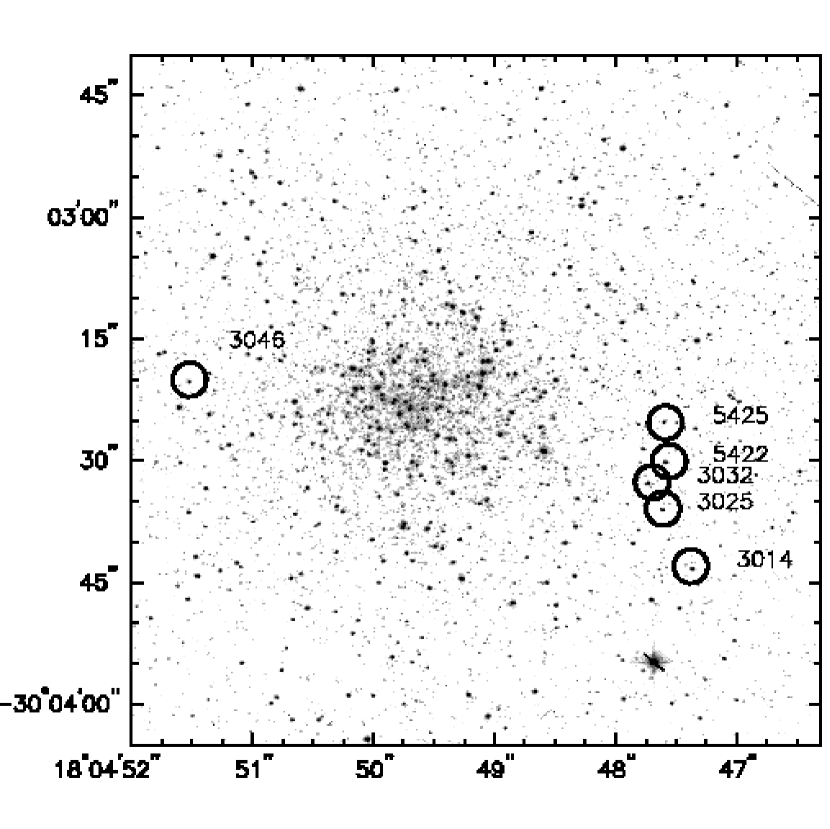
Figure 1: The stars in NGC 6528 studied here are marked on this subset from a 100 sec WFPC2 image from the HST Archive taken with the F555W filter.

Program stars were selected using high resolution images and VIJK photometry of NGC 6528 from HST (VI) and IRAC2 (JK) kindly provided by Montegriffo (1999, private communication). Table 1 gives the most relevant parameters of these stars, while Figure 1 shows their location within the cluster and Figure 2 the position of these objects in the $V,V-I$ color-magnitude diagram of NGC 6528. In Figure 1, the stars studied here are marked on this subset from a 100 sec WFPC2 image from the HST Archive. Coordinates for the program stars are given in Table 1. The field of the cluster is very crowded. We selected for observation a number of apparently uncrowded stars having colours and magnitudes appropriate for the RHB in the CMD, in order to maximize the probability of cluster membership. Beside the 4 program stars (namely, 5422, 3014, 3025 and 3046) two other stars fell in the edge of the slit (stars 3032 and 5425) on at least some of the spectra. While not good enough for abundance analysis, spectra of these extra stars are adequate for precise radial velocities. A posteriori, membership of the program stars in NGC 6528 was confirmed by their radial velocity: this is a very useful criterion in this case, due to the large $v_{r}$ of this cluster; according to Harris (1996), the heliocentric $v_{r}$ is $184.9\pm 3.8$ (internal error) km s^-1, and its $v_{r}$ relative to the Solar local standard of rest is 195 km s^-1. Heliocentric $v_{r}$ for the program stars as measured on our spectra are given in the column 6 of Table 1: the average heliocentric $v_{r}$ from our spectra is $209.9\pm 1.6$ km s^-1  with $\sigma=4.0$ km s^-1 from 6 stars, giving double weight to velocity from the June 2000 spectra that have a higher S/N ratio.

The radial velocities were measured by cross correlating the region 6130 - 6170 Å in echelle order 57 and the region 6240 - 6280 Å in echelle order 58, using the June 2000 spectrum of star 3025 as a template. These measurements were carried out independently and with different software packages by EC and by JC. The zero point was determined by fitting Gaussians to 16 lines in these orders in the spectrum of the template judged to be unblended based on their FWHM. The laboratory wavelengths of these lines were taken from the NIST Atomic Spectra Database. (NIST Standard Reference Database No. 78). The agreement between orders is excellent and confirms the dispersion solution from the Th-A lamp.

The internal radial velocity errors were calculated following the method of Tonry & Davis (1979) using the relation $\sigma(v_{r})=\alpha/[1+R(TD)]$, where the parameter $R(TD)$ is a measure of the ratio of the height of the peak of the cross correlation to the noise in the cross correlation function away from the peak. The constant $\alpha$ was set at 15 km s^-1, which represents a value typical of those found in other recent HIRES programs using similar instrumental configurations by Mateo et al. (1998), Cook et al. (1999), and Côté et al. (1999). The maximum error in $v_{r}$ incurred by a point source which is on the edge of the 1 arcsec slit compared to an object that uniformly fills the slit is 4 km s^-1, and this factor will be smaller for real stars under real seeing conditions that are partially in the slit. The systematic errors are thus generously set at 1.5 km s^-1 for the program stars observed in 2000, and 2.5 km s^-1 for the stars observed in 1999 as well as for those that fortuitously appeared in the slits.

Our velocity dispersion measured for NGC 6528 is by far the smallest published for this cluster, and is consistent with a normal mass-to-light ratio for NGC 6528. However, our mean $v_{r}$ is distinctly higher that the literature value in the compilation by Harris. A search of the references quoted by Harris revealed that all low values of $v_{r}$ for NGC 6528 are from older studies, while the most recent works tend to give a value quite similar to our own. For example, Minniti (1995) found an average $v_{r}$ of $203\pm 20$ km s^-1 from 7 stars, noting also that $v_{r}$ of this cluster was found to have some discrepancy in previous analyses (e.g. in Armandroff & Zinn 1988). The recent extensive work by Rutledge et al. (1997a) found $v_{r}$ = $212.2$ km s^-1 with $\sigma=13.5$ km s^-1 (external error) based on 8 stars. Both these results are in very good agreement with our $v_{r}$. We note that for NGC 6553, Rutledge et al. (1997a) found $v_{r}$ = 8.4 km s^-1 ($\sigma=8.4$ km s^-1), in quite good agreement with the value of Paper I. Moreover, Rutledge et al. (1997a) already noted that their high value for NGC 6528 was different at the 3.4$\sigma$ level from the mean value in Harris’ compilation and expressed concern about the potential impact on measurements of $v_{r}$ of possible non-members in clusters so heavily contaminated by field stars. This discussion further supports our adopted strategy of selecting target objects among the RHB stars.

The confirmation of this high $v_{r}$ is important as it is among the largest in absolute value for a bulge cluster so close to the galactic center. The radial velocity of NGC 6528 ($209.9\pm 1.6$ km/s) might be a reflection of the velocity dispersion of the metal rich bulge globular cluster population (Côté 1999) although it appears as rather extreme for a bulge object: in fact this value is slightly less than 2 $\sigma$ (of the scatter of values for individual field stars) from the mean value for bulge K-giants (Terndrup et al. 1995), M-giants (Sharples et al. 1990), RR Lyrae’s (Gratton et al. 1987), and Miras (Feast et al. 1980). While this large radial velocity clearly rules out the possibility that NGC6528 is a disk cluster, there is the possibility that it belongs to the inner halo rather than to the bulge and its orbit is by chance just passing through the bulge at the present time. The distinction between inner halo and bulge is not clearly defined at present. To obtain better insight into this issue, we examined more closely the large sample of bulge K-giants located in Baade’s Window, as is NGC 6528, observed by Terndrup et al.. We will consider only those stars fainter than $V=16$ (contamination by disk interlopers being important for brighter objects). For these stars, Terndrup et al. found an average velocity of $-8\pm 6$ km/s, with a dispersion of $110\pm 10$ for individual objects. 20 out 334 stars (that is, 6%) have radial velocities in excess of 200 km/s (in absolute value), i.e. have kinematics similar to or more extreme than that of NGC 6528. The average metallicity for these stars (Sadler et al. 1996) is [Fe/H]=$-0.17\pm 0.12$, with a scatter for individual stars of 0.53 dex. The average value is not significantly different from the average metal abundance they found for the whole sample of bulge K-giants ([Fe/H]=$-0.11\pm 0.04$). These stars are clearly much more metal-rich than the traditional value for halo stars ([Fe/H]$<-1$), and have a metal abundance quite similar to that we found for NGC6528. Note that these considerations are based on the high radial velocity of NGC 6528, which makes its membership in the disk population unlikely. On the other hand, the low radial velocity of NGC 6553 is compatible with that of a disk object. Some support for this view is given by a recent study by Beaulieu et al. (2001). Their color-magnitude diagram for NGC 6553 does not show a good match to the field bulge population and favors a metallicity comparable to solar, in good agreement with the revised value that we suggest in the present work (see below).

2.2 Details of the Observations

Observations were carried out with the HIRES spectrograph at Keck I. The HIRES detector is not large enough to yield full spectral coverage in a single exposure. The RHB stars in NGC 6528 are faint, and hence the exposures are long, so a single compromise instrumental configuration is mandatory. In our first effort described in Paper I, we wished to avoid crowding of lines, and hence centered the spectra rather far toward the red. It turned out that, ignoring Fe I absorption lines, there were few useful features beyond 8000 Å and also that line crowding was tolerable even at the blue end of the HIRES spectra of the RHB stars in NGC 6553. Thus for the observations of the NGC 6528 RHB stars, the instrumental configuration was set to shift the spectra blueward, so that the O triplet at 7770 Å appears in the reddest order included. This configuration had the advantage of adding features of several important elements with no lines in the wavelength regime covered in Paper I, such as Na, as well as important additional Fe II lines to improve the analysis of ionization equilibrium. However, the downside of this layout was that the unblended Mg I line at 8717 Å was lost, while the Mg I lines included in this setup are more blended and more saturated.

These fields are rather crowded. Given the freedom to rotate the slit to a desired position angle and the ability to track at a fixed position angle, in many cases it might be possible to get two or more candidate RHB stars within the length of the HIRES slit. At the time of our initial observations for NGC 6553, HIRES did not have an image rotator to compensate for the rotation of the field at the Nasmyth focus, and hence only one star could be observed at a time. However, by 1999, the HIRES image rotator had been completed by David Tytler and the Lick Observatory engineering group (Tytler 2000, private communication). The maximum slit length that can be used with our instrumental configuration without overlapping echelle orders is 14 arcsec. Leaving room at the ends of the slit for sky, we therefore searched the list of RHB candidates for suitable pairs of RHB candidates located not more than 7 arcsec apart.

The observations were carried out in two runs 10 months apart:

a) run of August 1999. Due to a hardware problem, the lower dome shutter of the Keck I telescope was not movable, and at low elevations it vignetted the telescope. This forced us to observe only one object in NGC 6528 per night, and that only during the hour centered on culmination of the cluster.

Exposures were 1200 sec, and 3 such were obtained for star 3014 and star 3025, while only two were obtained from 3046 and for 5422. The stars were dithered by one or two arcsec along the length of the slit between exposures.

b) Run of June 2000. Two exposures were obtained in NGC 6528 on the nights of June 2 and June 3, 2000 (i.e. 1 each night). Each was 7200 sec long, in 1200 sec segments, with small spatial dithers along the slit between each segment. Each exposure contained the RHB star 3025 and a second star, either 3014 or 5422. Thus the total exposure for star 3025 was 14,400 sec. The HIRES setup was identical for these two exposures. The S/N of these spectra, based strictly on the count rate in the continuum near the center of the echelle orders, is 65/pixel (130/4 pixel resolution element) for star 3025 and 95/4 pixel resolution element for the other two stars in NGC 6528.

The spectra from both runs were reduced using the suite of routines for analyzing echelle spectra written by McCarthy (1988) within the Figaro image processing package (Shortridge 1988). The stellar data are flat fielded with quartz lamp spectra, thereby removing most of the blaze profile, and the results are normalized to unity by fitting a 10th-order polynomial to line-free regions of the spectrum in each order.

2.3 The Measurement of Equivalent Widths

The spectra of the three stars observed in June, 2000 (stars 3014, 3025 and 5422) are of high S/N, and equivalent widths were measured directly from them; the August 1999 spectra were not used in the abundance analysis for these objects. However, star 3046 was only observed in 1999. The S/N of the 1999 spectra is not very large (typically $\sim 30$). For this star only, we followed the same procedure successfully used in Paper I to improve the reliability of measures of equivalent widths. We filtered the spectra by convolving them with a Gaussian having a FWHM of 0.3 Å (this reduced the resolution of the spectra down to $\sim 15,000$ but enhanced the S/N per pixel to about 60). We also applied the above procedure to the spectra of the 3 other stars of the 1999 run in order to derive a linear relationship between the two sets of measured EWs, and thus to correct the 1999 EWs of star 3046 measured using convolved spectra to that of the higher precision June, 2000 spectra:

$${\rm EW(2000)}=0.90{\rm EW(1999)}+12.5$$ (1)

with the correlation coefficient $r=0.93$ and $\sigma$=19.7 from 361 lines.

Since the spectra of the program stars are very line rich, the following procedure was adopted to measure reliable equivalent widths (EWs) on these spectra. First, we corrected the continuum slightly by using a spline interpolating function: appropriate “continuum” points were selected by comparing the spectra of different stars, so that the fiducial continuum level was set consistently for each star. This was done for all program stars. However, for star 3046, whose spectra are at somewhat lower resolution, greater care is needed. We then selected a small number of clean lines, and used these lines to set a fiducial relation between the FWHM of lines and their EWs. EWs for a larger number of lines were then measured by using a special fitting routine that measures EWs using this relation between FWHM and EWs, shown in Figure 3. With this scheme, the FWHM, which is very sensitive to the presence of blending lines, was constrained when measuring the EWs of individual lines, resulting in much more stable measures.

Note that for each line, the fitting routine used an interactively selected portion of the line profile, so that regions of the profile obviously disturbed by blending lines were not considered. In this way, we are not using just the central pixel, but a portion of the line profile that is generally broader than the FHWM of the line (by itself broader than a resolution element), and we are fitting the central part of the line adopting a model of the line profile which is a Gaussian, whose FWHM is a (linear) function of the EW. As also noted by the referee, it is however possible that EWs are somewhat overestimated. On the other side, since the continuum is likely to be somewhat underestimated, if the two effects are not mutually compensating, we should notice some trends of abundances as a function of the wavelength, and this is not the case.

Apart from errors due to the continuum placement and to blends, random errors $\delta$EW in these EWs are: $\delta$EW = $\frac{FWHM}{\sqrt{n}\cdot S/N}$, where n is the number of points used in the fitting, and S/N is per pixel. In our case n $\sim\frac{1.06\cdot FWHM}{dx}$ (actually, somewhat larger, in general), where dx is the wavelength step; that is, we may write: $\delta$EW = $\frac{1.06\cdot FWHM}{S/N*}$ where now S/N* is the S/N per FWHM element (generally larger than a resolution element).

Table 2 lists the final values of the EWs, along with the adopted $gf$ values. Errors in the EWs measured by this procedure may be estimated by comparing the EWs of different stars, since all four RHB stars have very similar atmospheric parameters (see below). Through such comparisons, we obtain typical rms scatters about the linear relationship between two stars of 9 mÅ. If we assume that both sets of EWs have equal errors, we can estimate that typical errors in EWs are 6 mÅ from the better quality spectra of June, 2000. These errors are mainly due to uncertainties in the positioning of the fiducial continuum. Errors in EWs measured on previous 1999 spectra (i.e. namely for star 3046) are somewhat larger, between 10 and 12 mÅ.

3 Abundance Analysis

3.1 Determination of Atmospheric Parameters

The analysis of the CMD of NGC 6528 (Ortolani et al. 1992) revealed that the interstellar reddening toward this cluster is quite large, somewhat uncertain, and with strong variations even within small projected distances on the sky. Infrared photometry by Cohen & Sleeper (1995) confirmed the presence of substantial reddening variations within this cluster. For this reason, it is not possible to derive accurate atmospheric parameters from the observed colours of stars in NGC 6528. Following the approach adopted in Paper I (where we had a similar problem), effective temperatures for the program stars were derived directly from the spectra, by forcing Fe I lines of different excitation to provide the same abundance (typically 90-100 Fe I lines were measured for each star, 70 for star 3046, with lower quality spectra). The errors on the linear regression fits allow one to estimate the (internal) errors in these temperatures: they are $\pm 85$ K (corresponding to 1$\sigma$ rms uncertainty of 0.017 dex/eV in the slope). As an example, left panels of Figure 4 shows the run of abundances from individual Fe I lines with excitation potential for the RHB stars. Systematic errors mainly depend on the set of model atmospheres used in the analysis (Kurucz, 1992: models with overshooting, for consistency with the analysis of Carretta & Gratton 1997). They are not easy to estimate, but we feel they are about $\pm 100$ K.

Observation at slightly shorter wavelengths than done in Paper I allowed a larger number of Fe II lines to be measured (typically at least 4 good Fe II lines for each star): we were then able to estimate surface gravities $\log g$ from the equilibrium of ionization of Fe. Internal errors in these surface gravities are $\pm 0.36$ dex (where we considered both the contributions due to errors in EWs of individual lines, and those due to uncertainties in the adopted $T_{\rm eff}$). Again systematic errors are mainly related to the adopted model atmospheres, and to the assumption of LTE made throughout this paper. (This seems a solid assumption for the stars we are currently considering: see Gratton et al. 1999). The average gravity we derived ($2.16\pm 0.14$) is very close to that predicted by evolutionary models for RHB stars in such a metal-rich cluster (about 2.3 dex, from the latest Padova isochrones, Salasnich et al. 2000), supporting the temperature scale adopted in the present analysis.

Microturbulent velocities $v_{t}$ were derived by eliminating any trend in the derived abundances from Fe I lines with expected equivalent widths for the lines (following the approach of Magain 1984). Given the large number of Fe I lines measured, internal error bars in these $v_{t}$’s are small ($\pm 0.12$ km/s). As an example, the central panels of Figure 4 show the run of abundances from individual Fe I lines with EWs for the four program stars.

Of course, it is well known that in abundance analyses the derived values of microturbulent velocity depend on the gf’s one is using. Our gf’s are obtained by combining mainly two sources (see Carretta & Gratton 1997, henceforth CG97, for detailed references): (i) for all strong lines, and a few of the weak ones, we are using laboratory gf’s from a compilation of data from the literature. Only gf’s with errors $<$0.05 dex were considered; (ii) for the vast majority of weak lines (most of the lines measurable in the spectra of NGC 6528 stars), we use solar gf’s, obtained from an inverse analysis whose zero point is set by the lines having laboratory gf’s (and whose abundance generally agree well with meteoritic values).

As noted also by the referee, there is some correlation between line strength and excitation potential ($\chi$), in the sense that there is a generic tendency of low-excitation Fe I lines to be stronger than those of high excitation. This is shown by the curves-of-growth in the right-handed panels of Figure 4, where open squares are used for lines with $\chi>3$ eV, while filled circles are for lines with $\chi\leq 3$ eV.

To test the relevance of this problem in our analysis, we repeated it, considering only those Fe I lines having $\chi>3$ eV; we did not changed the temperature since the excitation range included is now too small to allow fitting of $T_{\rm eff}$, but we re-optimized the microturbulent velocity. When only lines with $\chi>3$ eV are considered, we are essentially using only solar gf’s; these lines are weak in the solar spectrum, so that these gf’s are virtually independent of details in the solar analysis. The $v_{t}$ values we derived from this subset of lines are smaller than the original ones by $0.07\pm 0.06$ km/s, and the Fe abundances are larger by $0.03\pm 0.03$ dex. Both these values are barely significant and much lower than the other sources of errors.

The final adopted atmospheric parameters are shown in Table 3.

An analysis of the influence of errors on the derived abundances is given in Table 4. This table was obtained in the conventional way, specifically by comparing the abundances derived for star 3025 with those derived by varying the atmospheric parameters, one at a time, by the amount given in Table 4. As expected, larger effects arise from uncertainties in $T_{\rm eff}$ (in particular for neutral species) and in gravity (in particular for singly ionized species), whereas the overall metal abundance and the microturbulent velocity only play a minor role. The last column of Table 4 gives the quadratic sum of effects due to individual parameters listed; this can be taken as an estimate of the total uncertainty due to errors in atmospheric parameters. The uncertainty in O/Fe is by far the largest entry in this column.

3.2 Results

One of our goals is to extend the calibration of the metallicity scale for globular clusters of Carretta & Gratton (1997) to the metal-rich regime. Therefore for the sake of consistency we adopt the same atomic parameters (listed in Table 2) that they used, just as we did in Paper 1. Note that the only difference in the line lists used for NGC 6528 and NGC 6553 is in the slightly different wavelength region covered, due to the different instrumental configuration of HIRES used for the observations. However, both lists are simply subsets of that used in CG97, securing the required homogeneity. In addition, the same set of model atmospheres (Kurucz 1992 with convective overshooting), code for abundance analysis, etc. previously adopted are also used in the present work. Combining our previous work on NGC 6553 (Cohen et al. 1999) with the present study doubles the sample of clusters with metal abundances near the solar value, while retaining a highly homogeneous fine abundance analysis for all clusters studied to date.

From the four RHB stars, we find that the mean [Fe/H] for NGC 6528 is $+0.07\pm 0.01$ dex, with a star-to-star scatter of $\sigma=0.02$ dex. This is the first high dispersion analysis of a galactic globular cluster in which an abundance greater than solar has been obtained. Note however that the uncertainties are from statistics only. A fair estimate of the total error bar should include also systematic errors, that are in general rather hard to quantify: including systematics, a conservative budget could be about 0.1 dex, mostly due to errors related to the temperature scale and to adopted model atmospheres.

The resulting abundances for each species in each star are listed in Table 5. As in Paper I, all element ratios are computed with respect to Fe I, except for O I and Sc II where we used abundances from Fe II to minimize the uncertainties resulting from the choice of $T_{\rm eff}$. The rms dispersion in abundance among the measured set of lines for each ion is given in parentheses and the adopted solar abundances are shown in the last column of Table 5. The results for star 3046 are from EWs converted to the same system of the 3 other stars. Only abundances derived from at least 2 lines are shown for star 3046. Also, for comparison, we give in the last column of this Table the abundances obtained by a similar analysis of the well known population I star $\zeta$ Cyg from Paper I.

For oxygen and sodium (discussed in detail below), we give also the abundances (from line analysis) including corrections for departures from LTE, following Gratton et al. (1999).

Abundances for Sc II, V I and Mn I include detailed corrections for the quite large hyperfine structure of their lines (see Gratton 1989 and Gratton & Sneden 1991 for references).

The Ca abundances were derived applying to each line used the collisional damping parameter appropriate for that line (Smith & Raggett 1981).

An estimate of Eu abundance was obtained by comparing the average spectrum of all the RHB stars in NGC 6528 observed in the region of the Eu II line at 6645.11 Å with synthetic spectra (Figure 5). From this comparison, evidence for a mild ([Eu/Fe] $\simeq 0.2$) overabundance of Eu is found.

3.3 Checks on the derived metal abundances

A potential problem affecting the reliability of our results could be the contamination of Fe I lines by blends. McWilliam and Rich (1994) demonstrated that in bulge stars the effects of CN lines alone can be overwhelming at metallicities whose mean is similar to the values derived here. We expect this concern to be much less important in our spectra since they have a much higher resolution than those used by McWilliam and Rich and the temperature of the stars is higher. However, in order to check the impact of this problem, we considered more in detail the Fe I lines. For each Fe I line included, we synthesized a spectral region of 3.2 Å centered on the line, using line lists extracted from Kurucz 1995 CD-ROMs (CD-ROM 23 for the atomic lines; and CD-ROM 15 for diatomic molecules; note that these lists include lines due to CN as well as to other molecules) and the same model atmospheres used for the program stars. (In this exercise, we assumed [C/Fe]$-0.5$ and [N/Fe]$+0.5$ since, as reminded by the second referee, RHB stars have already experienced the phase along the red giant branch where C is usually depleted and N enhanced, and their sum is constant.). The synthetic spectra were then convolved with a Gaussian with a FWHM of 0.12 Å, in order to match the resolution of our spectra. We examined the profiles, and flagged all lines whose profiles are in some way distorted by blends; we then measured the EWs of the lines on these synthetic spectra using a Gaussian fitting routine (all parameters left free; EWs obtained by this procedure are much more affected by the presence of blends than those obtained using the procedure we applied for the program stars).

These EWs were then compared with those obtained from a spectral synthesis where the line list only consisted of the line under scrutiny (using this time a simple integration over the profile). Next we flagged all lines where the two EWs differ more than 2 mÅ (note that the weakest Fe I lines have EW$>40$ mÅ). Finally we adopted as very clean lines those with no appreciable distortion in the profiles, and for which the EWs are not changed by more than 2 mÅ by blends. We find a total of 53 very clean Fe I lines; such lines are marked with an asterisk in Table 2. Average abundances obtained from this subset of lines are within 0.020 dex of those derived from the original sample which in addition included lines of somewhat poorer quality. Furthermore the r.m.s. scatter of individual values are not modified in a significant way.

This exercise suggests that (i) the procedure used to measure EWs (i.e. adopting an average relation between EWs and FWHM to constrain the FWHM) allows us to derive reliable EWs even for moderately blended lines as in the spectrum of star 3046; and (ii) that the largest source of errors in the EWs is the location of the continuum level rather than the presence of blends.

Moreover, following the same procedure as in Paper I, we checked our overall [Fe/H] values by comparing our spectra with syntheses of a spectral region around the Li doublet, which includes several weak or medium strength Fe lines. These comparisons are shown in Figure 6, only for the 3 stars having new, high quality spectra from the run of 2000. The remaining star, 3046, was tied on the EW system defined from the 3 others as explained above.

The comparisons between the spectral syntheses and the observed spectra for the RHB stars in NGC 6528 shown in Figure 6 support the abundances found by the analysis of the equivalent widths. Lines computed with [Fe/H]=$-$0.13 and [Fe/H]=+0.27 are clearly too shallow and too strong with respect to the observations. Figure 6 also shows that no lithium is detectable in all our program stars. The synthetic spectra in Figure 6 are computed with log n(Li) = $-$2; however, since the Li line is blended with a Fe line, the upper limit determined from our spectra is log n(Li)$<0$.

We also note that if we only use Fe I lines with log(gf) - $\theta\chi\leq-7.2$ (where $\theta$ = 5040/T), which corresponds to the weakest lines that could be detected in the spectra taken in the June 2000 run, we obtain [Fe/H]=+0.08 dex using 14 lines for star 3025, [Fe/H]=+0.09 for star 5422 using 11 lines, and [Fe/H]=+0.06 for 12 lines in star 3014, which values are indistinguishable from those obtained with the full set of Fe I lines. Abundances from such weak lines are almost independent of the choice of microturbulent velocity. Although expected by the manner in which $v_{t}$ is set, the close agreement in the derived Fe abundance between the set of weak lines and the full set of Fe I lines is reassuring.

4 Discussion of Results

The present results are summarized in Table 6, where we list also the mean abundances for NGC 6553 (both from Paper I and from B99), and for 11 giants in Baade’s Window studied by McWilliam & Rich (1994), in order to provide a deeper insight into our findings. For NGC 6528 and our analysis of NGC 6553, if there was only one line per star for a given ion, the value is given in parentheses.

4.1 Comparisons of Fe Abundance

The most meaningful and immediate comparison is with our results for NGC 6553 from Paper I, since the analysis technique and data set are very consistent and homogeneous. However, both the quality of the observational material and the approach to the EW measurements present some differences.

Therefore, the first test we performed was a direct comparison of spectra of stars in the two clusters. RHB stars are objects in a well defined evolutionary phase. Hence, we can expect their stellar stucture and parameters to be very similar at similar metallicities.

This is evident from Figure 7, where the spectrum of star 71 in NGC 6553 (from Paper I) is compared to that of star 3025 of NGC 6528 (from the present work) in the spectral region 6700-6740Å. For a meaningful comparison, the spectra have been degraded to the same resolution. This Figure shows that spectra of the two stars are actually very similar, apart for some small differences in the positioning of the continuum. We conclude that the two stars can hardly be considered different or even distinguishable on the basis of their spectra.

This idea is strongly supported by Figure 8, where average EWs from stars of NGC 6553 (Paper I) and NGC 6528 (present study) are compared. In order to make the comparison more robust and less dependent on details of the continuum tracing, we average only EWs of lines measured in at least 3 stars out of 5 in NGC 6553 and in at least 2 stars out of the 3 with better quality spectra in NGC 6528.

Again, this comparison is quite good and EWs are quite similar for a hypothetical $average$ RHB star in the two clusters.

If the observed spectra are the same and the equivalent widths are very similar, then the difference of about 0.2 dex in the average overall metallicity of these two globular clusters ([Fe/H]$=-0.16$ for NGC 6553 and [Fe/H]$=+0.07$ dex in NGC 6528) must arise from the different atmospheric parameters adopted in the two analysis. In fact, both here and in Paper I, the atmospheric parameters adopted were derived directly from spectra, i.e. from EWs, that in turn were measured on spectra of different quality (better for the NGC 6528 stars observed in the run of June 2000) and using different methods.

To verify this, we use Table 4 to estimate the changes in [Fe/H] as due to differences between the mean atmospheric parameters used for RHB stars in NGC 6553 (namely 4727/2.3/$-$0.13/1.82 for temperature, gravity, model abundance and microturbulent velocity, respectively) and the mean set used for NGC 6528 (namely 4620/2.21/+0.07/1.34). The resulting difference in [Fe/H] is $-0.24$, in the sense that an $average$ star in NGC 6553 should be more metal-poor than the $average$ one in NGC 6528. The small difference in adopted microturbulence of only 0.5 km s^-1 gives rise to most of the abundance difference.

Another experiment seems to confirm this finding. We used the set of average EWs for NGC 6528 and repeated the analysis. We derive the values 4640/2.28/0.08/1.37 for $T_{\rm eff}$, $\log g$  [A/H] and $v_{t}$, and obtain [Fe/H]$=+0.08$ using the procedures discussed in Section 3.1 of zeroing trends of abundance from single lines with $\chi$ and expected line strengths. With these values we also obtained a very good ionization equilibrium.

If we now repeat the abundance analysis applying this set of atmospheric parameters to the average EWs of NGC 6553, we obtain a solution where the slopes of linear regressions of abundances $vs$ $\chi$ and of expected line strengths are well within the 1$\sigma$ rms uncertainty. The resulting abundance for NGC 6553 is then [Fe/H]$=+0.04$, i.e. we can conclude that an acceptable value for the overall metallicity of this cluster, as estimated from the Fe I abundance, is only 0.04 dex lower than that of NGC 6528.

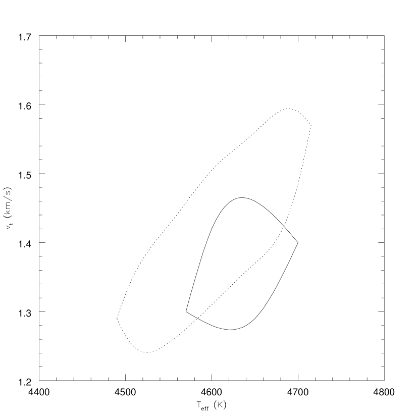
Figure 9: Parameter space $v_{t}$, $T_{\rm eff}$ in the range for RHB stars. The closed lines define the loci where solutions can be obtained with errors in slopes of linear regressions of abundances $vs$ $\chi$ and of expected line strengths within the 1$\sigma$ rms uncertainty. The dotted line refers to solutions for NGC 6553, while the solid one is for solutions valid for NGC 6528, for which higher quality spectra and EWs are available (see text).

Finally, Figure 9 shows the parameter space $v_{t}$, $T_{\rm eff}$ over the regime expected for RHB stars. Using the average EWs, we show the contours which give errors in slopes of linear regressions of abundances $vs$ $\chi$ and of expected line strengths within the 1$\sigma$ rms uncertainty. The loci for both NGC 6528 (solid line) and for NGC 6553 (dotted line) are elongated. This is simply another, graphic representation of the coupling that exists between $v_{t}$ and $T_{\rm eff}$ for cool, metal-rich stars discussed above (Section 3.1).

The higher quality spectra taken in the second run for NGC 6528 do alleviate this phenomenon, permitting high precision measurements of EWs of weak lines also of high excitation. This in turn allows us to better constrain the region of this parameter space within which solutions of the abundance analysis are acceptable.

These tests support the conclusion that within the error bars, the overall metal abundance of the two clusters expressed in terms of [Fe/H] is virtually the same. This is a firm result, since the number of measured Fe lines is large. Taking into account the overall uncertainty, we can be quite confident that NGC 6528 is a close “twin” of NGC 6553, as far as the overall metal abundance is concerned. Both these bulge clusters have a metallicity slightly larger than solar. Extremely high abundances for NGC 6528 as well NGC 6553 can be safely ruled out, as confirmed also by their normal integrated colours (see Figure 8 in Feltzig & Gilmore 2000).

To be conservative, we will adopt hereinafter a value of metallicity for NGC 6553 that is the mean of that obtained in Paper I, and the one obtained with atmospheric parameters equal to those of NGC 6528. As error bar, we will adopt one giving these two values as extremes of our confidence range. Hence, we will adopt for NGC 6553 a value of [Fe/H]$=-0.06\pm 0.15$ dex.

4.2 Comparison With NGC 6553 For Other Elements

The pattern described by the element ratios appears to be rather similar for the two clusters. The average abundances are generally in good agreement, apart for the [Mg/Fe] ratio. However, as discussed in §2.2, with the present instrumental set up, we had no access to the Mg line at 8717.8 Å, the clean line used in the analysis of RHB stars in NGC 6553. Instead we had to use two lines around 5600 Å that are located in a more crowded region and are saturated, hence not optimal for a good abundance derivation. Even if the abundance from the line at 7657 Å that we measured for stars observed in the 2000 run generally confirms results from the other lines, at present, and until further confirmation, we cannot be very confident that the low Mg abundance found for NGC 6528 is real.

The overabundance of Si and of Ca seems to be well established in NGC 6528. Since, however, O abundances (discussed later) and Ti abundances seems more likely solar, it is not clear that NGC 6528 presents the classical overabundance of the $\alpha$-elements typical of more metal-poor clusters and field stars.

On the other hand, Mn is rather underabundant in NGC 6528, and this result is a signature of a small contribution to nucleosynthesis by SN Ia, suggesting that the $\alpha$-elements overabundance might be the typical fossil record of a nucleosynthesis history heavily dominated by massive stars. Some support to this scenario could be given by the mild overabundance of Eu found from the combined spectrum of the RHB stars in NGC 6528, since Eu is known to be a n-capture element predominantly produced by r-processes. Note however that the ratio [Ba/Eu] is almost solar, suggesting that maybe we are seeing also the contribution to nucleosynthesis from intermediate-mass stars.

A comparison of our results for NGC 6553 with those of B99 was given in section 7.1 of Paper I. Here, we note only that the choice of solar and stellar atmosphere model adopted in B99 (hence the solar abundances) results in Fe abundances that are 0.1 to 0.15 dex lower than those of the present scale. This by itself decreases the differences in the element ratios presented in Table 6. In other words, had the comparison for NGC 6553 been made, instead, in terms of [element/H], the pattern of many elements would have been more similar when our analysis of Paper I was compared to that of B99.

4.3 O and Na Abundances

The slightly different instrumental configuration of HIRES adopted for the observations of the RHB stars in NGC 6528 allowed the use of the weak Na doublet at 6154, 6160 Å as well as the infrared permitted O I triplet, and, for three of the four stars, the forbidden 6300 Å O I line as well.

To take into account departures from the adopted assumption of LTE, appropriate corrections were applied to O and Na abundances following the prescriptions of Gratton et al. (1999). Non-LTE abundances from the line analysis are also listed in Table 5. Note however, that the corrections are rather small, and do not exceed a few hundredths of a dex in all cases.

We tested the abundances we derived for Na and O using synthetic spectra of the 6154-60 Na I doublet, and of the [O I] line at 6300 Å. The spectral synthesis were computed assuming LTE. Comparisons with spectral synthesis for these two spectral regions are shown in Figures 10 and 11 respectively.

From the comparisons in Figure 10 we found that Na is overabundant by about +0.35 to +0.5 dex in stars 3025, 5422, and 3014 (respectively, we estimated [Na/Fe]= +0.5, +0.35 and +0.4 dex). These results are consistent with that deduced from the EWs.

The comparison between observed and synthesized spectra for the region including the [OI] line at 6300.3 Å is more difficult for three reasons. First, there are several telluric lines in this region whose locations are marked with a T in Figure 11. Due to the high $v_{r}$ of NGC 6528, the wavelength of the [OI] line in the observed spectra of NGC 6528 is free of contamination by telluric lines; they should not affect our results. Second, as mentioned in Section 3.1, O abundances are quite sensitive to uncertainties in the atmospheric parameters. Third, there is some coupling between C and O abundances, due to formation of CO in the atmospheres of these cool, metal-rich K-giants. We estimated that derived O abundances increase by 0.06 dex if the C abundances are raised by 0.2 dex. Unfortunately, we could not determine C abundances from our spectra, since EWs of C I lines measured in the red are not reliable; we can only fix the overall strength of CN lines. We matched adequately CN lines by assuming [C/Fe]=$-$0.45 and [N/Fe]=0 when [O/Fe]=$-$0.07; [C/Fe]=$-$0.3 and [N/Fe]=0 when [O/Fe]=0.13; and [C/Fe]=$-$0.18 and [N/Fe]=0 when [O/Fe]=+0.33. These are the values adopted in the syntheses shown in Figure 11.

Figure 11 shows that with the adopted C and N abundances, a good fit of the [OI] line is obtained for [O/Fe]$\sim 0$, in reasonable agreement with the results given by the analysis of the equivalent widths (where also other O lines are taken into account). An O excess of 0.3 dex seems excluded, unless the C abundance is not much larger than solar, which seems unlikely.

We conclude that the program stars in NGC 6528 have solar oxygen abundances, but a distinct excess of Na ([Na/Fe]$\sim 0.4$).

4.4 Metal Abundances: Calibration of Other Indices

Our need, after the completion of our analysis of NGC 6553 of Paper I, to have an analysis for stars in at least one more metal-rich cluster is apparent if one examines Figure 12, where the metallicities obtained from high resolution spectra by CG97, plus those for NGC 6553 and NGC 6528 (this study) are plotted against the parameter W(CaII) determined by Rutledge et al. (1997) from the measured strength of the infrared Ca triplet in individual globular cluster giants.

For reasons explained in Section 4.1, we believe that the correct [Fe/H] values to adopt for these two clusters are +0.07 and $-$0.06 dex for NGC 6528 and NGC 6553, respectively.

When NGC 6528, which has the largest value of any galactic globular cluster observed to date on the Rutledge et al. ranking scale (W(CaII)=5.41), is added, the conclusion proposed in Paper I is still firmly supported. Specifically, the two scales seem to be linearly correlated over the range from [Fe/H]$=-2.2$ to [Fe/H]$=-0.6$ (i.e. up to not so extremely metal rich clusters). At higher metallicities, however, where the CaII index is known to lose its sensitivity to metal abundance (see Armandroff & Da Costa 1991), the linear correlation seems to break down.

Note that clusters like Pal 12 or Rup 106, known to have anomalously low [$\alpha$/Fe] ratios, are not included in the sample.

With our new results we can now better assess the relationship between the two scales: in fact, NGC 6528 falls very near NGC 6553, in the [Fe/H]–W(CaII) plane, and strongly constrains the position of metal-rich globular clusters for the metallicity calibration in terms of this low resolution indicator. This is not unexpected, since in Section 4.1 we showed how RHB stars of these 2 clusters are similar. We find that to bring the values from Rutledge et al. onto a homogeneous metallicity scale which is based completely on high dispersion spectroscopy, one has to adopt a second order polynomial relation:

$${\rm[Fe/H]_{us}}=-2.08-0.04{\rm W(CaII)}+0.078{\rm W^{2}(CaII)}$$ (2)

with the correlation coefficient $r=0.98$ and $\sigma$=0.12 dex for 22 clusters. The second order term is significant at a confidence level exceeding 95%; inclusion of this term yields $\chi^{2}=25.8$ for the sample of 22 globular clusters in common. This is a reduction in $\chi^{2}$ of a factor of 1.6 compared to a linear fit. Notice that similar results are obtained even if we omit entirely NGC 6553, so that the larger error bar of the revised [Fe/H] value for this cluster does not affect much our calibration.

This relation, shown in Figure 12, allows us to derive directly from the Ca index of a globular cluster its metallicity on the Carretta & Gratton scale, as extended here and in Paper I. The range of application should be restricted to that of calibrating clusters, namely from W(CaII) $\sim 1.5$ (NGC 7078,NGC 4590) to W(CaII) $\sim 5.4$ (NGC 6528). Moreover, using data from the compilation of Carney (1996), we checked that the differences between the W(CaII) values as observed by Rutledge et al. and the W(CaII) values predicted from our eq. (2) are constant as a function of [Ca/Fe]. We can then conclude that, since the [Ca/Fe] ratio holds rather constant for all clusters in the sample, we are actually calibrating an index that is tied to the temperatures and luminosities of stars along the RGB, which in turn depend on the cluster metal abundance.

Adding a second well analyzed high metallicity cluster is also very useful in intercomparing the CG97 scale and the widely used scale of Zinn & West (1984) (based on integrated light indices). We are now able to derive a relation to bring their values on the new scale entirely based on high dispersion analyses, without using any uncertain extrapolations. As in CG97, we prefer to use directly final metallicities from Zinn & West (1984), with the update of Armandroff & Zinn (1988; collectively ZW), due to the variety of indicators used in the analysis of Zinn & West (1984).

When NGC 6528 and NGC 6553 are added to the other 24 calibrating clusters, the quadratic relation previously found by CG97 is no longer the most appropriate, as one can see in Figure 13, where mean metallicities from the CG97 scale as augmented here are compared with metallicities on the ZW scale.

In this case a cubic polynomial is the best relation to transform the ZW scale to the new high dispersion spectroscopic scale:

$${\rm[Fe/H]_{CG}}=+0.61+3.04{\rm[Fe/H]_{ZW}}+1.981{\rm[Fe/H]_{ZW}}^{2}+0.532{\rm[Fe/H]_{ZW}}^{3}$$ (3)

with $\sigma$=0.10 dex and a correlation coefficient $r=0.99$ for 26 clusters.

When considering the adopted error bar of 0.15 dex for the revised value of [Fe/H] of NGC 6553, the second and third order terms are significant at the 99% confidence level.

The value of $\chi^{2}$ decreases by more than a factor of two in going from a linear fit to a third order fit, e.g. from 392 to 144 for the comparison of our abundances with those of Zinn & West (1984) for the 26 clusters (25 without NGC 6553) in the sample with high dispersion abundance analyses.

The present work extends the range of application of this transformation by about 0.3 dex toward high metallicity, with respect to eq. 7 in CG97. Using the above relation now allows one to transform the ZW metallicities onto our high dispersion scale in the range $-2.24<$[Fe/H]${}_{\rm ZW}<+0.12$.

5 Conclusions

We present for the first time an abundance analysis for stars in the metal-rich bulge cluster NGC 6528 based on high resolution spectra of S/N high enough to allow a reliable fine abundance analysis.

We observed 4 red HB stars, from which we found a mean [Fe/H]$=+0.07\pm 0.01$ dex, with a star-to-star scatter of $\sigma=0.02$ (not including systematic effects).

This metallicity is slightly larger than the mean abundance in the galactic bulge found by McWilliam & Rich (1994), and that found in a previous paper for NGC 6553. However, we found that the spectra of stars in NGC 6553 and NGC 6528, and the EWs we measured on them, are very similar to each other. The slightly different metal abundance is the result primarily of adoption of slightly lower microturbulent velocity in the analysis of NGC 6528 stars and secondarily of the adoption of slightly lower temperatures for the NGC 6528 stars.

Note that the present analysis is based on higher quality spectra, so that the atmospheric parameters here used for NGC 6528 are more firmly established than those used in Paper I for NGC 6553.

If the same atmospheric parameters are adopted for both samples, nearly equal metal abundances are derived for the two clusters. We then propose to revise upward the metal abundance of NGC 6553 to [Fe/H]$=-0.06\pm 0.15$, where the error bar encompasses both the original abundance for NGC 6553 we derived in Paper I, and the value we obtained assuming in the analysis atmospheric parameters identical to those we used for stars in NGC 6528.

These results imply that metal-rich globular clusters may reach or even exceed the mean abundance of the galactic bulge found by McWilliam & Rich, but are found to fall within the spread of their distribution.

The relative abundance for the best determined $\alpha$-process elements (Ca) indicates an excess of $\alpha$ process elements of about a factor of two and a global pattern of abundances similar to that of NGC 6553 and the bulge field stars. Moreover, Mn in NGC 6528 clearly shows an underabundance typical of a quite small contribution to nucleosynthesis by yields from SN Ia. When coupled with the overabundances of Si and Ca, our results strongly suggest that these bulge globular clusters seem to have experienced a history of chemical enrichment essentially identical to that typical of bulge field stars, probably under conditions of enrichment by type II Supernovae at early epochs.

We found a solar O abundance, while there is a clear excess of Na ([Na/Fe]$\sim 0.4$). However the sample is not large enough to understand if this abundance pattern is characteristics of all stars in this cluster, or rather stems from peculiarities of the program stars or their evolutionary state.

Our new data for NGC 6553 (Paper I) and NGC 6528 allow us to re-calibrate the widely used metallicity scales of Zinn & West (1984) and of Rutledge et al. (1997), both based on low dispersion or integrated indices, onto a scale fully based on high dispersion spectroscopy. We give the functions required to transform W(CaII) and [Fe/H]_ZW values into our updated scale, superseding the previous calibration by Carretta & Gratton (1997).

Appendix A The Reddening of NGC 6528

Like other bulge clusters heavily reddened and/or affected by differential reddening, the value of E(B-V) for NGC 6528 in the literature ranges over more than 0.2 mag, e.g. 0.46 mag (Richtler et al. 1998) from $V,I$ photometry, 0.55 mag (Ortolani et al. 1992 and Zinn 1980), and 0.73 mag from cluster integrated colours (Reed et al. 1988).

Since an underestimate of 0.05 mag in the value of E(B-V) translates into an underestimate of about 0.2 dex in metal abundance when temperatures are derived from colours (Cohen 1983), this issue deserve special care. Even methods such as that of Sarajedini (1994), which uses fits to the shapes of unreddened giant branches to derive metallicity and reddening simultaneously, are unreliable for very metal-rich clusters, since the most metal-rich of his calibrating clusters is 47 Tuc ([Fe/H]$=-0.70$).

With the present analysis, we have a spectroscopic determination of the temperatures of four RHB stars that are derived only from the excitation of many Fe I lines. These estimates are therefore reddening-free and provide an independent route to the value of E(B-V) in NGC 6528.

As a starting point we assumed a mean value of $T_{\rm eff}\sim$ 4610 K as representative of the spectroscopic temperatures of our RHB stars (see Table 3). This temperature, with the mean metallicity and gravity from Table 3, corresponds to a value (V-K)${}_{0}=2.53$ based on the colour–$T_{\rm eff}$ calibration of Gratton, Carretta & Castelli (1997). On the other hand, from the V,K photometry of Montegriffo (1999) the mean V-K colour for the 4 program stars is 3.88; so that, assuming a standard relation E(V-K)=2.7 E(B-V) (e.g. Cardelli et al. 1989), we deduce a value of E(B-V) = 0.50 mag as an independent estimate for the reddening of NGC 6528. Repeating the above exercise using the $individual$ colours and parameters of each star, we could not isolate any significant difference in the resulting values of E(B-V).

This value is somewhat lower than the one listed in the compilation by Harris (1996), as well most of the values quoted above, although only slightly smaller that that found in the field just N and W of the cluster by Stanek (1996). (Stanek’s value in the field just S of the cluster is close to that of Harris.) We believe that this arises because of a selection bias. In a metal-rich globular cluster with differential reddening, the RHB shape in a CMD changes from the normal short horizontal one characteristic of a constant reddening to an extended distribution sloping towards fainter magnitudes for the redder stars. Such a RHB is clearly shown in the case of NGC 6553 in Figure 2b of Ortolani et al. (1990) and NGC 6528 (in Figure 2). Our sample of RHB stars selected for high dispersion spectroscopy is biased towards the brighter stars, and hence the less reddened ones. Table 3 shows, however, that the program stars have a total range in $T_{\rm eff}$ of 70 K (well within the adopted uncertainties), even though they cover a rather large range in the observed reddened CMD.

NGC 6528 is known to be affected by differential reddening. Cohen & Sleeper (1995) establish that the range of E(B-V) is about 0.25 mag. Consistent with the suggestion of differential reddening, it is interesting to note that three of the program stars are located in the same region of NGC 6528. For differential reddening of the magnitude found in NGC 6528, this selection effect far outweighs any tendency toward picking RHB stars that are slightly evolved off the zero age HB.

Irrespective of the origin of this effect and of the mean value of E(B-V) for NGC 6528, we stress here that the determination of temperatures by line excitation is a purely spectroscopic, reddening-free method and that this is the method used for the four RHB stars we observed.

As noted by the referee, one may wonder how sensitive this method could be to errors in gf values. In previous section, we performed a test aimed to understand if our values for the microturbulent velocity were biased due to the correlation existing between line strength and excitation potential, because lines of low excitation are all strong. Hence we compared the values for the $v_{t}$ derived from all lines with those we derive using only high excitation lines. This second value is nearly independent of the assumed temperature, because all lines have nearly the same excitation potential.

We checked the zero-point of this calibration using field red clump stars (Carretta et al., Cohen et al. in preparation) with atmospheric parameters similar to those of stars in NGC 6528 and with good parallaxes from Hipparcos. These stars are sufficiently close that it is reasonable to assume that the reddening is negligible.

Table 1: The Sample of Stars Observed in NGC 6528

ID	$V$	$I$	$J$	$K$	$v_{r}$	Date of Obs.	Exp. Time	Coord.
	(mag)	(mag)	(mag)	(mag)	(km s-1)		(sec)	(J2000)
Red HB Stars
5422	16.95	15.34	14.11	13.14	$206.8\pm 1.0\pm 2.5$	990817	2 X 1200	18 04 47.58 $-$30 03 30
					$206.4\pm 0.7\pm 1.5$	000603	6 X 1200
3025	17.14	15.43	14.21	13.22	$218.1\pm 1.0\pm 2.5$	990817	3 X 1200	18 04 47.62 $-$30 03 36
					$216.8\pm 0.7\pm 1.5$	000603	12 X 1200
3014	17.09	15.38	14.21	13.21	$212.0\pm 1.0\pm 2.5$	990815	3 X 1200	18 04 47.38 $-$30 03 43
					$205.7\pm 0.7\pm 1.5$	000603	6 X 1200
3046	17.25	15.50	14.12	13.34	$207.3\pm 1.0\pm 2.5$	990818	2 X 1200	18 04 51.52 $-$30 03 20
5425	17.09	15.35	14.25	13.32	$209.2\pm 0.8\pm 2.5$	000603	$<2500$	18 04 47.62 $-$30 03 25
3032	16.69	14.71	13.58	12.34	$211.2\pm 0.8\pm 2.5$	000603	$<2500$	18 04 47.34 $-$30 03 33

Table 2: Equivalent Widths For 4 Red HB Stars in NGC 6528

Ion	$\lambda$ (Å)	$\chi$ (eV)	$\log(gf)$	5422		3025		3014		3046
				(mÅ)		(mÅ)		(mÅ)		(mÅ)
O I	6300.31	0.00	$-$9.75		40.0		39.0		37.0
O I	6363.79	0.02	$-$10.25		9.0		15.0		13.0
O I	7771.95	9.11	0.33		40.0		36.0		35.0		54.8
O I	7775.40	9.11	$-$0.03		30.0		31.0
Na I	5682.65	2.10	$-$0.67		182.9		194.4		200.7
Na I	5688.22	2.10	$-$0.37		184.8		187.1		208.6
Na I	6154.23	2.10	$-$1.57		114.5		125.3		116.5		101.6
Na I	6160.75	2.10	$-$1.26		140.8		137.2		142.9		119.6
Mg I	5528.42	4.34	$-$0.62		270.1		264.5		276.3
Mg I	5711.09	4.34	$-$1.83		156.6		157.5		155.0		132.0
Mg I	7657.60	5.11	$-$1.28		124.5		115.7		165.9
Si I	5645.62	4.93	$-$2.14		84.4				96.2
Si I	5665.56	4.92	$-$2.04		93.5		80.3		99.5		78.2
Si I	5684.49	4.95	$-$1.65		75.8		95.1		112.5
Si I	5690.43	4.93	$-$1.87		75.7		95.3		78.8		90.2
Si I	5701.11	4.93	$-$2.05		61.5		73.1
Si I	5708.41	4.95	$-$1.47		129.8
Si I	5772.15	5.08	$-$1.75		95.1		103.0		83.9		87.2
Si I	5793.08	4.93	$-$2.06		91.8		99.2		94.8
Si I	5948.55	5.08	$-$1.23		127.4		117.2		133.9		108.7
Si I	6125.03	5.61	$-$1.57		69.6		59.9		60.7		54.5
Si I	6145.02	5.61	$-$1.44		51.6		56.2		59.2		51.9
Si I	6848.57	5.86	$-$1.75		50.5		47.2		42.7
Si I	6976.50	5.95	$-$1.17				83.8
Si I	7003.58	5.96	$-$0.87				63.9		70.2
Si I	7034.90	5.87	$-$0.88		93.7		86.0		110.2
Si I	7226.20	5.61	$-$1.51								60.6
Si I	7405.79	5.61	$-$0.82		111.4		120.7		126.6
Ca I	5590.13	2.51	$-$0.57		128.1				150.9
Ca I	5594.47	2.51	0.10		224.5		215.0		213.1
Ca I	5857.46	2.93	0.24		182.9		178.4		208.0		184.3
Ca I	5867.57	2.93	$-$1.49		66.7		75.2		86.8		62.8
Ca I	6161.30	2.52	$-$1.27		122.1		129.0		114.0
Ca I	6166.44	2.52	$-$1.14		107.4		120.0		122.5		119.7
Ca I	6169.04	2.52	$-$0.80		145.0		142.9		150.7
Ca I	6169.56	2.52	$-$0.48		164.5		164.3		160.9
Ca I	6439.08	2.52	0.39								234.9
Ca I	6462.57	2.52	0.26		299.3		282.5		299.7
Ca I	6471.67	2.52	$-$0.69		152.9		153.1		162.8		128.5
Ca I	6493.79	2.52	$-$0.11		174.9		185.3		197.4		193.0
Ca I	6499.65	2.52	$-$0.82		130.7		144.6		147.7		145.7
Ca I	6572.80	0.00	$-$4.32								139.7
Ca I	6717.69	2.71	$-$0.52		197.9
Sc II	5526.82	1.77	0.19		140.0		127.2		128.6
Sc II	5640.99	1.50	$-$0.86		103.4		101.5
Sc II	5657.88	1.51	$-$0.29		119.4		121.5		120.6
Sc II	5667.15	1.50	$-$1.11		80.8		81.5
Sc II	5669.04	1.50	$-$1.00		86.8		81.0		92.3		64.8
Sc II	5684.20	1.51	$-$0.92				82.6		102.4
Sc II	6245.62	1.51	$-$1.05		88.1		89.6		98.1		79.2
Sc II	6604.60	1.36	$-$1.14		88.7		92.8		100.9		89.8
Ti I	5490.16	1.46	$-$0.93		97.1		101.3		87.7
Ti I	5503.90	2.58	$-$0.19		81.9
Ti I	5662.16	2.32	$-$0.11				87.8		102.1
Ti I	5689.48	2.30	$-$0.47						57.4		60.4
Ti I	5866.46	1.07	$-$0.84		144.6		139.3		160.9		123.3
Ti I	5922.12	1.05	$-$1.47		102.5		111.7		106.3		90.8
Ti I	5978.55	1.87	$-$0.58		105.5		96.3		108.0
Ti I	6091.18	2.27	$-$0.42		68.2		69.9
Ti I	6126.22	1.07	$-$1.42		93.1		104.9		107.9		87.9
Ti I	6258.11	1.44	$-$0.36		122.7		131.7		134.7
Ti I	6261.11	1.43	$-$0.48		166.8				157.2
Ti I	6554.24	1.44	$-$1.22								109.2
Ti I	7251.72	1.43	$-$0.84		122.7		126.3		125.2		148.7
V I	5627.64	1.08	$-$0.37								103.8
V I	5670.86	1.08	$-$0.42		116.1		110.7		105.0		87.1
V I	5703.59	1.05	$-$0.21		111.3		113.8		113.9
V I	5727.06	1.08	$-$0.01								142.6
V I	6081.45	1.05	$-$0.58		98.9		95.2		116.8
V I	6090.22	1.08	$-$0.06		120.8		115.0		130.6
V I	6119.53	1.06	$-$0.32								107.4
V I	6199.19	0.29	$-$1.28		141.5		134.0		148.7
V I	6216.36	0.28	$-$1.29								138.5
V I	6243.11	0.30	$-$0.98						180.6
V I	6251.83	0.29	$-$1.34		116.2		117.2		116.9		113.6
Cr I	5409.80	1.03	$-$0.71				268.1
Cr I	5702.33	3.45	$-$0.68				76.6		76.1
Cr I	5781.19	3.32	$-$0.88		79.4		64.1		55.6
Cr I	5781.76	3.32	$-$0.75		81.1		67.5		69.1
Cr I	5783.07	3.32	$-$0.40						59.6		53.6
Cr I	5783.87	3.32	$-$0.30				96.0		89.5		97.8
Cr I	5784.98	3.32	$-$0.38		89.6		80.5		96.9
Cr I	5787.93	3.32	$-$0.08		97.5		80.9		82.8
Cr I	6330.10	0.94	$-$2.87								115.1
Cr I	6882.50	3.44	$-$0.38				65.8
Cr I	6883.07	3.44	$-$0.42		65.6		64.2		71.9
Cr I	6882.52	3.44	$-$0.38				65.8
Cr I	6883.06	3.44	$-$0.42		65.6		64.2		71.9
Cr I	6979.80	3.46	$-$0.22		76.0		86.8		77.0
Cr I	6980.94	3.46	$-$1.09		40.3
Cr I	7400.19	2.90	$-$0.11		132.6		151.6		151.8		162.5
Cr II	5502.09	4.17	$-$1.96		46.0		46.1
Cr II	5508.63	4.15	$-$2.07		57.7		38.7		53.3
Mn I	5394.67	0.00	$-$3.50				199.7
Mn I	5420.37	2.14	$-$1.46				192.9
Mn I	5432.55	0.00	$-$3.80		176.1		188.4
Mn I	6013.50	3.07	$-$0.25								146.1
Mn I	6016.65	3.07	$-$0.09								146.2
Mn I	6021.80	3.08	0.03		183.7		133.7		165.4		150.7
Mn I	7302.85	4.43	$-$0.37		59.5		58.8		52.0
Fe I	5386.34*	4.15	$-$1.74				70.7
Fe I	5389.49	4.41	$-$0.57				105.5
Fe I	5395.22	4.44	$-$1.73				49.0
Fe I	5398.29*	4.44	$-$0.72				100.7
Fe I	5406.78	4.37	$-$1.40				65.7
Fe I	5412.79	4.43	$-$1.80				57.6
Fe I	5417.04	4.41	$-$1.42				67.0
Fe I	5436.30	4.39	$-$1.36		77.8
Fe I	5464.29	4.14	$-$1.62		60.4		75.0
Fe I	5470.09*	4.44	$-$1.60		57.0		55.7
Fe I	5491.84	4.19	$-$2.24		48.1		36.5		39.0
Fe I	5494.47	4.07	$-$1.96		61.1		68.9		63.6
Fe I	5522.45*	4.21	$-$1.47		89.3		86.9		91.0
Fe I	5560.22*	4.43	$-$1.10		71.9		80.1
Fe I	5577.03*	5.03	$-$1.49				33.1
Fe I	5587.58	4.14	$-$1.70		72.6				84.3
Fe I	5618.64	4.21	$-$1.34				90.2		100.0		66.0
Fe I	5619.61	4.39	$-$1.49		68.6						59.5
Fe I	5650.00	5.10	$-$0.80				69.0		65.3
Fe I	5651.48*	4.47	$-$1.79				39.2
Fe I	5661.35	4.28	$-$1.83				64.9		55.4
Fe I	5701.56	2.56	$-$2.16		156.5		151.0		163.1
Fe I	5717.84	4.28	$-$0.98								89.3
Fe I	5731.77*	4.26	$-$1.10		101.6		86.7		103.1
Fe I	5738.24	4.22	$-$2.24		50.8		40.9		50.9
Fe I	5741.86*	4.26	$-$1.69				61.5		73.9		71.2
Fe I	5752.04*	4.55	$-$0.92		73.2		82.3		86.0		87.3
Fe I	5760.36	3.64	$-$2.46		62.8		67.3		77.0
Fe I	5775.09	4.22	$-$1.11		95.6		105.9		97.2
Fe I	5778.46	2.59	$-$3.44		82.2		76.0		76.8
Fe I	5784.67*	3.40	$-$2.53		77.0		73.2
Fe I	5793.92*	4.22	$-$1.62				78.5		77.2
Fe I	5835.11	4.26	$-$2.18						58.1
Fe I	5852.23	4.55	$-$1.36								75.9
Fe I	5855.09*	4.61	$-$1.56		54.1		47.9				33.6
Fe I	5856.10*	4.29	$-$1.57				75.2				61.9
Fe I	5858.78	4.22	$-$2.19		36.8		49.0		41.9		46.3
Fe I	5859.60	4.55	$-$0.63		97.5		105.5		118.4		89.5
Fe I	5862.37*	4.55	$-$0.42		110.9		108.5		128.3		102.6
Fe I	5881.28	4.61	$-$1.76				41.3
Fe I	5905.68	4.65	$-$0.78								71.2
Fe I	5927.80	4.65	$-$1.07		66.5		79.9		69.9		54.7
Fe I	5929.68*	4.55	$-$1.16		83.2		75.3		71.9
Fe I	5930.19*	4.65	$-$0.34		121.8		123.3		126.2		110.1
Fe I	5934.66	3.93	$-$1.08		121.0		117.1		123.0		123.8
Fe I	5956.71*	0.86	$-$4.56		129.1		137.2				128.4
Fe I	5976.79*	3.94	$-$1.30		111.1		109.5		109.1
Fe I	6003.02	3.88	$-$1.02								123.1
Fe I	6027.06*	4.07	$-$1.20		99.5		103.7		119.5		117.3
Fe I	6056.01	4.73	$-$0.46		88.0		104.5		102.8		110.9
Fe I	6065.49*	2.61	$-$1.49		189.6		192.7		199.9
Fe I	6078.50*	4.79	$-$0.38		100.9		106.9		111.3
Fe I	6079.02*	4.65	$-$0.97		75.9		80.9		95.0
Fe I	6082.72	2.22	$-$3.53		108.1				104.9
Fe I	6089.57	5.02	$-$0.87		69.7		70.5		78.0
Fe I	6093.65*	4.61	$-$1.32		64.5		73.5
Fe I	6094.38	4.65	$-$1.56						53.4
Fe I	6096.67*	3.98	$-$1.76		89.6		78.1		87.3
Fe I	6098.25	4.56	$-$1.81				42.5		50.0
Fe I	6137.00	2.20	$-$2.91		147.6				155.7
Fe I	6151.62*	2.18	$-$3.26		109.3		114.5		115.5		115.5
Fe I	6157.73	4.07	$-$1.26								120.6
Fe I	6165.36	4.14	$-$1.48		85.0		86.9		90.6		63.4
Fe I	6173.34*	2.22	$-$2.84		138.1		148.6		149.0		139.7
Fe I	6187.99	3.94	$-$1.60		99.1		89.4		93.8
Fe I	6200.32*	2.61	$-$2.39		144.9		146.6		158.4
Fe I	6219.29	2.20	$-$2.39								169.4
Fe I	6232.65	3.65	$-$1.21		115.2		140.2		133.5
Fe I	6240.65	2.22	$-$3.23		109.7				116.1
Fe I	6246.33*	3.60	$-$0.73		146.7		158.2		156.0		145.9
Fe I	6252.56*	2.40	$-$1.64						206.1
Fe I	6265.14	2.18	$-$2.51								187.6
Fe I	6270.23	2.86	$-$2.55		115.4		102.8		116.5		102.2
Fe I	6297.80*	2.22	$-$2.70		157.9				156.1
Fe I	6301.51*	3.65	$-$0.72		161.0		162.2		178.5
Fe I	6322.69	2.59	$-$2.38								135.4
Fe I	6330.85	4.73	$-$1.22								65.5
Fe I	6335.34	2.20	$-$2.28								175.4
Fe I	6380.75	4.19	$-$1.34		100.4		98.5		104.5		110.6
Fe I	6392.54*	2.28	$-$3.97		69.0				92.4
Fe I	6400.32	3.60	$-$0.23		211.9		226.6		241.2
Fe I	6411.66	3.65	$-$0.60		155.9		166.3		171.8
Fe I	6421.36	2.28	$-$1.98		194.2		206.6		229.0
Fe I	6481.88	2.28	$-$2.94		143.9		142.7				123.1
Fe I	6498.95	0.96	$-$4.66		133.7		136.1		151.2		155.9
Fe I	6518.37*	2.83	$-$2.56		111.7		109.6		112.3
Fe I	6533.94	4.56	$-$1.28		80.8				73.6
Fe I	6574.25*	0.99	$-$4.96								104.3
Fe I	6581.22	1.48	$-$4.68						119.3		103.8
Fe I	6593.88*	2.43	$-$2.30		164.9		164.0		171.0		168.0
Fe I	6608.04	2.28	$-$3.96		67.2		76.2		75.9		66.3
Fe I	6625.04	1.01	$-$5.32						117.1		123.7
Fe I	6627.56	4.55	$-$1.50				58.5		62.9
Fe I	6633.76*	4.56	$-$0.81		94.3
Fe I	6703.58	2.76	$-$3.00		84.1		98.1				88.1
Fe I	6713.74	4.79	$-$1.41		58.7				49.2
Fe I	6725.36*	4.10	$-$2.21		41.9						46.6
Fe I	6726.67*	4.61	$-$1.05		82.5		77.6		88.2		74.5
Fe I	6733.15	4.64	$-$1.44		55.5		53.8		50.6		67.4
Fe I	6750.16*	2.42	$-$2.58		144.7		152.3		162.0		146.5
Fe I	6786.86*	4.19	$-$1.90		64.6		55.9		58.6
Fe I	6806.86	2.73	$-$3.14								109.0
Fe I	6810.27	4.61	$-$1.00								100.6
Fe I	6820.37	4.64	$-$1.16								81.9
Fe I	6837.01	4.59	$-$1.71		42.9		58.1		46.2
Fe I	6839.84	2.56	$-$3.35		95.6		97.0		98.3		106.1
Fe I	6843.66	4.55	$-$0.86		85.0				100.9		92.7
Fe I	6858.16	4.61	$-$0.95				79.1				97.7
Fe I	6861.95	2.42	$-$3.78		67.0		77.6		84.4
Fe I	6898.29	4.22	$-$2.08		44.4		43.8		64.2
Fe I	6916.69	4.15	$-$1.35		82.3		99.5		113.5
Fe I	6945.20	2.42	$-$2.46								175.0
Fe I	6951.25	4.56	$-$1.05								99.8
Fe I	6971.94*	3.02	$-$3.34		63.4		60.7		64.1
Fe I	6978.86	2.48	$-$2.49				142.3		143.0
Fe I	6988.53*	2.40	$-$3.42		108.2		103.4		108.4		109.3
Fe I	7007.97	4.18	$-$1.80		65.0		60.7		64.7		82.0
Fe I	7010.35	4.59	$-$1.86				46.7				52.1
Fe I	7022.96*	4.19	$-$1.11		110.9		100.2		108.6		106.2
Fe I	7024.07	4.07	$-$1.94				78.3
Fe I	7090.39	4.23	$-$1.06								133.6
Fe I	7114.56*	2.69	$-$3.93		46.5
Fe I	7118.10*	5.01	$-$1.52				35.4
Fe I	7132.99	4.07	$-$1.66		81.9		87.2		89.3
Fe I	7142.52	4.95	$-$0.93						81.9		89.1
Fe I	7151.47	2.48	$-$3.58		101.2				107.0		101.3
Fe I	7189.16*	3.07	$-$2.77				90.7
Fe I	7284.84	4.14	$-$1.63		89.7				96.1
Fe I	7306.57	4.18	$-$1.55		78.8		82.5		93.0
Fe I	7401.69	4.19	$-$1.60		71.2				93.5		100.2
Fe I	7411.16	4.28	$-$0.48		153.3		153.6
Fe I	7418.67	4.14	$-$1.44		78.5		85.3		91.1		103.0
Fe I	7421.56*	4.64	$-$1.69		37.3						36.0
Fe I	7430.54*	2.59	$-$3.82		80.5		79.4		91.1
Fe I	7447.40	4.95	$-$0.95				60.7				63.0
Fe I	7461.53	2.56	$-$3.45				85.0				100.2
Fe I	7491.66	4.30	$-$1.01		99.6				111.2
Fe I	7540.44	2.73	$-$3.75								74.2
Fe I	7547.90	5.10	$-$1.11								44.1
Fe I	7568.91*	4.28	$-$0.90		121.2				133.2		125.7
Fe I	7582.12*	4.95	$-$1.60				30.0
Fe I	7583.80	3.02	$-$1.93		150.8		149.4		165.5		171.2
Fe I	7719.05*	5.03	$-$0.96				55.0				64.9
Fe I	7723.21	2.28	$-$3.62		100.3				108.2		111.9
Fe I	7745.52	5.08	$-$1.14								65.0
Fe I	7751.11*	4.99	$-$0.74		82.6		85.6		94.8
Fe I	7807.91	4.99	$-$0.51		84.5		93.1
Fe II	5414.08	3.22	$-$3.61				42.4
Fe II	5425.26	3.20	$-$3.27		55.4		61.0
Fe II	5991.38	3.15	$-$3.55				62.9		65.1
Fe II	6084.10	3.20	$-$3.80						52.9
Fe II	6149.25	3.89	$-$2.72		52.6		50.0		51.7		52.0
Fe II	6247.56	3.87	$-$2.32		61.5		65.0		69.1		74.3
Fe II	6369.46	2.89	$-$4.21		27.2		30.2		36.5		40.2
Fe II	6416.93	3.89	$-$2.70		52.4		60.1
Fe II	6432.68	2.89	$-$3.58								67.7
Fe II	6516.08	2.89	$-$3.38						98.9		77.2
Ni I	5468.11	3.85	$-$1.63		28.8				31.0
Ni I	5578.73	1.68	$-$2.57		122.5		130.1		137.1
Ni I	5587.87	1.93	$-$2.39		116.4		125.9		124.5
Ni I	5593.75	3.90	$-$0.78		66.0		66.4
Ni I	5643.09	4.16	$-$1.25				33.7
Ni I	5748.36	1.68	$-$3.25		98.6		101.4		102.3
Ni I	5760.84	4.10	$-$0.81		82.8		77.6		73.1
Ni I	5805.23	4.17	$-$0.60		82.3
Ni I	5847.01	1.68	$-$3.44		92.6		94.1		103.2
Ni I	5996.74	4.23	$-$1.06		74.8		47.8				41.7
Ni I	6053.69	4.23	$-$1.07		54.9		75.6		78.9
Ni I	6086.29	4.26	$-$0.47		70.4		73.4		89.4
Ni I	6108.13	1.68	$-$2.47								151.1
Ni I	6111.08	4.09	$-$0.83								75.0
Ni I	6128.98	1.68	$-$3.39		100.4		97.1		96.3		74.2
Ni I	6130.14	4.26	$-$0.98						51.3		26.6
Ni I	6176.82	4.09	$-$0.24		100.2		100.7		106.6
Ni I	6177.25	1.83	$-$3.60		70.6				69.5
Ni I	6186.72	4.10	$-$0.90		67.4		57.8		65.7
Ni I	6204.61	4.09	$-$1.15		60.6		59.1		63.6
Ni I	6327.60	1.68	$-$3.08								122.7
Ni I	6378.26	4.15	$-$0.82		62.7		67.5		64.7		55.6
Ni I	6384.67	4.15	$-$1.00		63.4		72.1		61.5
Ni I	6482.81	1.93	$-$2.78		105.0		108.7		125.4		112.6
Ni I	6532.88	1.93	$-$3.42		82.2		88.2		84.5
Ni I	6586.32	1.95	$-$2.78		111.7		111.6		110.0		104.8
Ni I	6598.61	4.23	$-$0.93		50.9		45.9		55.7
Ni I	6635.14	4.42	$-$0.75		65.8		60.0		48.2		77.2
Ni I	6767.78	1.83	$-$2.06		140.7		153.3		161.9
Ni I	6772.32	3.66	$-$0.96		84.0		88.9		107.9
Ni I	6842.04	3.66	$-$1.44		66.5		71.3		67.7
Ni I	7001.55	1.93	$-$3.65		64.3		61.7		67.8		49.7
Ni I	7030.02	3.54	$-$1.70		46.3						50.7
Ni I	7034.38	3.54	$-$2.10		61.5		48.6		59.7
Ni I	7110.91	1.93	$-$2.91		132.5		130.5		122.3		116.6
Ni I	7327.65	3.80	$-$1.75		36.7		38.2
Ni I	7381.94	5.36	$-$0.05								30.3
Ni I	7401.12	5.36	$-$0.18		51.7		46.5
Ni I	7422.29	3.63	$-$0.29		146.9		160.6		157.9		162.9
Ni I	7525.12	3.63	$-$0.67								119.0
Ni I	7555.61	3.85	$-$0.12								134.8
Ni I	7574.05	3.83	$-$0.61		108.1		118.3		114.9		131.4
Ni I	7715.58	3.70	$-$0.98								110.6
Ni I	7727.62	3.68	$-$0.30		127.5		124.3		135.0
Ni I	7797.59	3.30	$-$0.82		125.1				123.8
Ni I	7863.79	4.54	$-$0.94								54.2
Zn I	6362.35	5.79	0.14		67.3		60.9		77.1
Y II	5509.91	0.99	$-$1.01		110.7		121.6
Ba II	5853.69	0.60	$-$1.00		127.2		127.5		129.7		126.1
Ba II	6141.75	0.70	0.00		169.4		184.3		199.7		155.4
Ba II	6496.91	0.60	$-$0.38		171.0		185.3		177.9		199.7

Table 3: Adopted Model Atmosphere Parameters

Star ID	$T_{\rm eff}$	log(g)	$v_{t}$
	(K)	(dex)	(km s-1)
Red HB Stars
5422	4580	2.3	1.25
3025	4650	2.3	1.32
3014	4630	2.0	1.45
3046	4580	2.0	1.34

Table 4: Sensitivity of Abundances To Atmospheric Parameters

	$\Delta T_{\rm eff}$	$\Delta logg$	$\Delta[A/H]$	$\Delta v_{t}$	Total
Change	+100 K	+0.2 dex	+0.1 dex	+0.2 km s-1
[O/Fe]	$-$0.352	$-$0.131	$-$0.142	$-$0.073	0.41
[Na/Fe]	0.000	$-$0.058	$-$0.030	$-$0.003	0.06
[Mg/Fe]	0.050	$-$0.078	0.037	0.047	0.11
[Al/Fe]	$-$0.125	$-$0.078	$-$0.063	$-$0.013	0.16
[Si/Fe]	$-$0.100	0.019	0.008	0.045	0.11
[Ca/Fe]	0.062	$-$0.040	$-$0.021	$-$0.035	0.08
[Sc/Fe]II	0.123	$-$0.031	$-$0.009	$-$0.008	0.13
[Ti/Fe]I	0.134	$-$0.016	$-$0.018	$-$0.014	0.14
[V/Fe]	0.128	$-$0.013	$-$0.028	$-$0.039	0.14
[Cr/Fe]	0.083	$-$0.012	$-$0.013	0.029	0.09
[Mn/Fe]	0.037	$-$0.028	$-$0.005	$-$0.033	0.06
[Fe/H]I	0.050	0.018	0.013	$-$0.087	0.10
[Fe/H]II	$-$0.123	0.111	0.042	$-$0.062	0.18
[Ni/Fe]	$-$0.027	0.034	0.008	$-$0.001	0.04
[Ba/Fe]II	$-$0.050	0.042	0.020	$-$0.093	0.12

Table 5: Abundances for Four Red HB Stars in NGC 6528

Ion		Star 5422			Star 3025			Star 3014			Star 3046			$\zeta$ Cygni			log n
		# of	abundance		# of	abundance		# of	abundance		# of	abundance		# of	abundance		(sun)
		lines	(dex)		lines	(dex)		lines	(dex)		lines	(dex)		lines	(dex)
[Fe/H]
Fe I		93	+0.05 (0.16)		100	+0.08 (0.11)		90	+0.09 (0.14)		70	+0.04 (0.24)		27	+0.05 (0.20)		7.50
Fe II		5	+0.12 (0.14)		7	+0.15 (0.16)		6	+0.15 (0.21)		5	+0.10 (0.04)		1	$-$0.06		7.44
[El/Fe]
O I		4	+0.18 (0.29)		4	+0.15 (0.12)		3	$-$0.08 (0.05)								8.62
O I (nLTE)		4	+0.16 (0.27)		4	+0.13 (0.11)		3	$-$0.09 (0.03)					3	+0.38 (0.18)		8.62
Na I		4	+0.44 (0.13)		4	+0.51 (0.16)		4	+0.54 (0.16)		2	+0.19 (0.01)					6.33
Na I (nLTE)		4	+0.42 (0.12)		4	+0.47 (0.16)		4	+0.51 (0.15)		2	+0.20 (0.04)					6.33
Mg I		3	+0.11 (0.17)		3	+0.05 (0.20)		3	+0.27 (0.25)					1	+0.20		7.54
Si I		14	+0.44 (0.25)		14	+0.39 (0.20)		13	+0.37 (0.22)		7	+0.24 (0.12)		2	+0.11 (0.26)		7.54
Ca I		13	+0.23 (0.26)		11	+0.27 (0.14)		12	+0.28 (0.18)		8	+0.14 (0.17)		3	+0.07 (0.04)		6.16
Sc II		5	$-$0.07 (0.06)		6	$-$0.09 (0.08)		5	+0.09 (0.06)		3	$-$0.13 (0.31)		1	+0.12		2.96
Ti I		10	+0.08 (0.29)		9	+0.08 (0.10)		10	+0.05 (0.25)		6	$-$0.08 (0.30)		1	$-$0.28		4.98
V I		6	$-$0.20 (0.13)		6	$-$0.25 (0.14)		6	$-$0.08 (0.21)		6	$-$0.29 (0.25)					4.00
Cr I		9	+0.05 (0.25)		13	+0.01 (0.22)		11	$-$0.06 (0.23)		4	+0.00 (0.39)		1	+0.02		5.62
Mn I		1	$-$0.39		4	$-$0.42 (0.18)					3	$-$0.29 (0.14)					5.39
Ni I		36	+0.15 (0.21)		32	+0.14 (0.20)		31	+0.05 (0.17)		20	+0.06 (0.29)		9	$-$0.08 (0.17)		6.25
Ba II		3	+0.18 (0.20)		3	+0.24 (0.14)		3	+0.08 (0.01)		3	+0.07 (0.38)					2.21

Table 6: Mean Abundances for NGC 6528 and Comparison With Results For NGC 6553 and For Baade’s Window

Ion	NGC 6528	$\sigma$	NGC 6553	$\sigma$	NGC 6553	$\sigma$	Mean BW	$\sigma$
			Paper I		Barbuy et al.
	(dex)	(dex)	(dex)	(dex)	(dex)	(dex)	(dex)	(dex)
[Fe/H]
Fe I	+0.07	0.02	$-$0.16	0.08	$-$0.55	0.20	$-$0.33
Fe II	+0.13	0.02	$-$0.18	0.10
[El/Fe]
O I	+0.07	0.11	+0.50	0.13			+0.03	0.18
Na I	+0.40	0.12			+0.65	0.05	+0.21	0.37
Mg I	+0.14	0.09	(+0.41)	(0.10)	+0.33	0.13	+0.35	0.14
Si I	+0.36	0.07	+0.14	0.18	+0.35	0.05	+0.18	0.24
Ca I	+0.23	0.06	+0.26	0.09	+0.32	0.12	+0.14	0.17
Sc II	$-$0.05	0.10	($-$0.12)	(0.18)			+0.29	0.20
Ti I	+0.03	0.07	+0.19	0.06	+0.51	0.09	+0.34	0.10
V I	$-$0.20	0.09					+0.06	0.19
Cr I	0.00	0.04	+0.04	0.09			$-$0.04	0.19
Mn I	$-$0.37	0.07
Ni I	+0.10	0.05	+0.01	0.07			$-$0.04	0.08
Ba II	+0.14	0.07			$-$0.10	0.30	+0.20	0.28

Figure 2: $V,V-I$ color-magnitude diagram of NGC 6528. Stars studied in the present work are indicated with larger, filled dot and labelled in Figure. Note that stars 3032 and 5425 were not used in the abundance analysis, due to the low S/N of their spectra.

Figure 3: Fiducial relation between the FWHM of lines and their EWs for star 3046, observed at lower resolution.

Figure 4: Abundances deduced from neutral Fe I lines as a function of excitation potential of the lower level of the transition (panels on the left) and of the equivalent widths (central panels) for the NGC 6528 RHB stars. In the panels on the right, curves-of-growth are also displayed, with open squares for lines with $\chi>3$ eV and filled circles for lines having $\chi\leq 3$ eV.

Figure 5: Comparison between the observed spectrum in the region of the Eu II line at 6645.11 Å(average of all stars in NGC 6528: thick line) and synthetic spectra computed for [Eu/Fe]= 0.0. 0.25, 0.50 (thin lines). From this comparison, evidence for a mild ([Eu/Fe] $\simeq 0.2$) overabundance of Eu is found.

Figure 6: Spectral synthesis of the region around the Li doublet for the 3 RHB stars of NGC 6528 with spectra taken in the run of June 2000. Thick lines are the observed spectra, while the thin lines are predictions for model atmospheres, with the parameters indicated in each box, for abundances of [Fe/H] listed at the bottom of each panel. Wavelengths have been shifted into the rest frame.

Figure 7: Comparison of spectra of two RHB stars in NGC 6553 (star 71, see Paper I; light line) and in NGC 6528 (star 3025, from present work; heavy line). Spectra have been degraded to the same resolution.

Figure 8: Comparison of average EWs for RHB stars in NGC 6553 and NGC 6528. The average is from the 5 stars studied in Paper I and is shown when a line is measured in at least 3 stars, for NGC 6553; for NGC 6528, the average was done using the 3 stars with spectra taken in the 2000 run and only if a line was measured in at least 2 stars.

Figure 10: Spectrum synthesis of the region of Na doublet at 6154 and 6160 Å for the RHB stars analyzed in NGC 6528 (only for stars observed in 2000). Thick lines are the observed spectra, while the thin lines are predictions for abundances of [Na/Fe] = 0.0, 0.2 and 0.4 dex.

Figure 11: Spectrum synthesis of the region of the [O I] forbidden line at 6300 Å of stars in NGC 6528 observed in the 2000 run. Thick lines are the original observed spectra, while the thin lines denote predictions for abundances of [O/Fe] = $-0.07$, 0.13, and 0.33 dex. The spectra were computed assuming [C/Fe] = $-0.45$, $-0.30$, and $-0.18$, and [N/Fe]=0; these choices reproduce the strength of the CN lines. T’s mark telluric features.

Figure 12: The parameter $W(CaII)$ defined by Rutledge et al. (1997b) is shown as a function of abundance on the scale of Carretta & Gratton (1997) for galactic GCs with high dispersion analyses, as updated by the analysis by Cohen et al. (1999) for NGC 6553 (but see text, Section 4.3) and the present study for NGC 6528. The dashed line is a linear fit, shown for comparison purposes. The solid line is the transformation adopted (see text).

Figure 13: The new calibration of the metallicity scale by Zinn & West (1984) against metal abundances from high dispersion spectroscopy. The dashed and solid lines have the same meaning as in the previous figure.

References

- (1) Armandroff, T.E. & Da Costa, G.S., 1991, AJ, 101, 1329
- (2) Armandroff, T.E. & Zinn, R., 1988, AJ, 96, 92
- (3) Barbuy, B., Renzini, A., Ortolani, S., Bica, E. & Guarnieri, M. D., 1999, A&A, 341, 539
- (4) Beaulieu, S.F., Gilmore, G., Elson, R.A.W., Johnson, R.A., Santiago, B., Sigurdsson, S. & Tanvir. N., 2001, AJ, 121, 2618
- (5) Bertelli, G., Bressan, A., Chiosi, C., Fagotto, F. & Nasi, E., 1994, A&AS, 106, 275
- (6) Cardelli, J. A., Clayton, G. C. & Mathis, J. S., 1989, ApJ, 345, 245
- (7) Carretta, E. & Gratton, R.G., 1997, A&A Supl, 121, 95
- (8) Cohen, J. G., 1983, ApJ, 270, 654
- (9) Cohen, J. G., Gratton, R.G., Behr, B.B. & Carretta, E. 1999, ApJ, 523, 739 (Paper I)
- (10) Cohen, J. G. & Sleeper, E. C., 1995, AJ, 109, 242
- (11) Cook, K., Mateo, M., Olszewski, E.W., Vost, S.S., Stubbs, C. & Diercks, A., 1999, PASP, 111, 306
- (12) Côté, P., 1999, AJ, 118, 406
- (13) Côté, P., Mateo, M., Olszewski, E.W. & Cook, K.H., 1999, ApJ, 526, 147
- (14) Davidge, T.J., 1999, astro-ph/9909408
- (15) Davis, M. & Tonry, J.L., 1977, AJ, 84, 1511
- (16) Feast, M.W., Robertson, B.S.C., & Black, C., 1980, MNRAS, 190, 227
- (17) Feltzig, S. & Gilmore, G. 2000, Astro-ph/0002123
- (18) Gratton, R. G., 1987, MNRAS, 224, 175
- (19) Gratton, R. G., 1989, A& A, 208, 171
- (20) Gratton, R. G., Carretta, E. & Castelli, F., 1996, A& A, 314, 191
- (21) Gratton, R. G., Carretta, E., Eriksson, K. & Gustafsson, B., 1999, A&A, 350, 955
- (22) Gratton, R.G. et al., 2001, A& A, 369, 87
- (23) Gratton, R. G., Sneden, C., 1991, A& A, 241, 501
- (24) Harris, W.E. 1996, AJ, 112, 1487
- (25) Ivans, I.I., Sneden, C., Kraft, R.P., Suntzeff, N.B., Smith, V.V., Langer, G.E. & Fullbright, J.P. 1999, AJ, 118, 1273
- (26) Kraft, R. P., Sneden, C., G Smith, G. H., Shetrone, M. D. & Fulbright, J., 1998, AJ, 115, 1500
- (27) Kurucz, R. L., 1992, CD-ROM 13
- (28) Magain, P., 1984, A&A, 134, 189
- (29) Mateo, M., Olszewski, E.W., Vogt, S.S. & Keane, M.J., 1998, AJ, 116, 2315
- (30) McCarthy, J. K., 1988, PhD thesis, California Institute of Technology
- (31) McWilliam, A. & Rich, R. M., 1994, ApJS, 91, 749
- (32) Minniti, D., 1995, A&A Suppl., 113, 299
- (33) Ortolani, S., 1999, invited talk, in The Chemical Evolution of the Galaxy: Stars versus Clusters, Vulcano, September 1999, in press
- (34) Ortolani, S., Barbuy, B. & Bica, E., 1990, A&A, 236, 362
- (35) Ortolani, S., Bica, E. & Barbuy, B., 1992, A&A Suppl, 92, 441
- (36) Ortolani, S., Renzini, A., Gilmozzi, R., Marconi, G., Barbuy, B., Bica, E. & Rich, R.M. 1995, Nature, 377, 701
- (37) Reed, B.C., Hesser, J. E. & Shawl, S. J., PASP, 100, 545
- (38) Rich, R. M., 1988, AJ, 95, 828
- (39) Rich, R. M. & McWilliam, A., 2000, to appear in SPIE, 4005 (ed. J.Bergeron). (Astro-ph/0005113)
- (40) Richtler, T., Grebel, E.K., Subramaniam, A., Sagar, R., 1998, A&AS, 127, 169
- (41) Rutledge, G. A., Hesser, J. E., Stetson, P. B., Mateo, M., Simard, L., Bolte, M., Friel, E. D. & Copin, Y., 1997a, PASP, 109, 883
- (42) Rutledge, G. A., Hesser, J. E.& Stetson, P. B., 1997b, PASP, 109, 907
- (43) Sadler, E. M., Rich, R. M., & Terndrup, D. M., 1996, AJ, 112, 171
- (44) Salasnich, B., Girardi, L., Weiss, A. & Chiosi, C., 2000, in preparation
- (45) Sarajedini, A. 1994, AJ, 107, 618
- (46) Sharples, R., Walker, A., & Cropper, M., 1990, MNRAS, 246, 54
- (47) Shortridge, K. 1988, “The Figaro Manual Version 2.4”
- (48) Smith, G., & Ragget, D. St. J., 1981, J. Phys. B. At. Mol. Phys., 14, 4015
- (49) Stanek, K.,1996, ApJ, 460, L37
- (50) Terndrup, D. M., Sadler, E. M., Rich, R. M., 1995, AJ, 110, 1774
- (51) Ventura, P., D’Antona, F., Gratton, R.G.,2001, ApJ, 550, L65
- (52) Vogt, S.E., Allen, S., Bigelow, B., Bresee, L., Brown, B., Cantrall, T., Conrad, A., Couture, M., Delaney, C., Epps, H., Hilyard, D., Hilyard, D., Horn, E., Jern, N., Kanto, D., Keane, M., Kibrick, R., Lewis, J., Osborne, C., Osborne, J., Pardeilhan, G., Pfister, T., Ricketts, T., Robinson, L., Stover, R., Tucker, D., Ward, J. & Wei, M., 1994, SPIE, 2198, 362
- (53) Zinn, R. J., 1980, ApJS, 42, 19
- (54) Zinn, R. & West, M. 1984, ApJS, 55, 45
- (55)