Gauge-ready formulation of the cosmological kinetic theory
in generalized gravity theories

Abstract

We present cosmological perturbations of kinetic components based on relativistic Boltzmann equations in the context of generalized gravity theories. Our general theory considers an arbitrary number of scalar fields generally coupled with the gravity, an arbitrary number of mutually interacting hydrodynamic fluids, and components described by the relativistic Boltzmann equations like massive/massless collisionless particles and the photon with the accompanying polarizations. We also include direct interactions among fluids and fields. The background FLRW model includes the general spatial curvature and the cosmological constant. We consider three different types of perturbations, and all the scalar-type perturbation equations are arranged in a gauge-ready form so that one can implement easily the convenient gauge conditions depending on the situation. In the numerical calculation of the Boltzmann equations we have implemented four different gauge conditions in a gauge-ready manner where two of them are new. By comparing solutions solved separately in different gauge conditions we can naturally check the numerical accuracy.

PACS numbers: 98.80.Cq, 98.80.Hw, 98.70.Vc, 04.62+v

]

I Introduction

The relativistic cosmological perturbation plays a fundamental role in the modern theory of large-scale cosmic structure formation based on the gravitational instability. Due to the extremely low level anisotropies of the cosmic microwave background (CMB) radiation, the cosmological dynamics of the structures in the large-scale and in the early universe are generally believed to be operated as small deviations from the homogeneous and isotropic background world model. The relativisitic cosmological perturbation analysis works as the basic framework in handling such cosmological structure formation processes. Recent observations of the CMB anisotropies in the small-angular scale by Boomerang and Maxima-1 experiments [1, 2], for example, confirm dramatically the validity of the basic assumptions used in the cosmological perturbation theory, i.e., the linearity of the relevant cosmic structures.

Soon after the discovery of the CMB by Penzias and Wilson in 1965 [3], Sachs and Wolfe in 1967 [4] pointed out that the CMB should show the temperature anisotropy caused by photons traveling in the perturbed metric which is associated with the large-scale structure formation processes based on the gravitational instability. The detailed dynamics at last scattering is not important in the large angular scale which can be handled using the null geodesic equations. Whereas, the physical processes of last scattering including the recombination process are important in the small angular scale where we need to solve the Boltzmann equations for the photon distribution function [5]. When we handle the evolutions of the collisionless particles, like the massive/massless neutrinos or the collisionless dark matters, we need the corresponding Boltzmann equations as well.

The relativistic gravity theory, including Einstein’s general theory of relativity as a case, is a non-Abelian gauge theory of a special type. The original perturbation analysis was made by Lifshitz in 1946 based on Einstein gravity with the hydrodynamic fluid [6]. In handling the gauge degrees of freedom arising in the perturbation analyses in the relativistic gravity, Lifshitz started by choosing the synchronous gauge condition and properly sorted out the remaining gauge degrees of freedom incompletely fixed by his gauge condition. Other approaches based on other (more suitable) gauge conditions were taken by Harrison using the zero-shear gauge in 1967 [7] and by Nariai using the comoving gauge in 1969 [8]. Each of these two gauge conditions completely removes the gauge degrees of freedom. Now, we know that the zero-shear gauge is suitable for handling the gravitational potential perturbation and the velocity perturbation, and the comoving gauge is suitable for handling the density perturbation. Since each of these two gauge conditions completely fixes the gauge transformation properties, all the variables in the gauge condition are the same as the gauge-invariant ones: that is, each variable uniquely corresponds to a gauge-invariant combination of the variable concerned and the variable used in the gauge condition.

The gauge-invariant combinations were explicitly introduced by Bardeen in 1980 [9]; see also Lukash 1980 [10] for a parallelly important contribution. This became a seminal work due to a timely introduction of the early inflation scenario [11] which provides a casual mechanism for explaining the generation and evolution of the observed large-scale cosmic structures. We believe, however, a practically more important suggestion concerning the gauge issue was made by Bardeen in 1988 [12], and it was elaborated in [13]. In the gauge theory it is well known that proper choice of the gauge condition is often necessary for proper handling of the problem. Either by fixing certain gauge conditions or by choosing certain gauge-invariant combinations in the early calculation stage we are likely to lose possible advantages available in the other gauge conditions. According to Bardeen “the moral is that one should work in the gauge that is mathematically most convenient for the problem at hand”. In order to use the various gauge conditions as advantages in handling cosmological perturbations we have proposed a gauge-ready method which allows the flexible use of the various fundamental gauge conditions. In this paper we will elaborate further the gauge-ready approach for more general situations of the generalized gravity theories including components described by the relativistic Boltzmann equations.

Our formulation is made based on the gauge-ready approach; using this approach our new formulation of the cosmological perturbation is more flexible and adaptable in practical applications compared with previous works. Also, the formulation is made for a Lagrangian which is very general, thus includes most of the practically interesting generalized versions of gravity theories considered in the literature. We pay particular attention to make the contribution of the kinetic components in the context of the generalized gravity theories. As an application of our gauge-ready approach made in this paper, we implemented the numerical integration of Boltzmann equations for CMB anisotropies in four different gauge conditions. In addition to the previously used synchronous gauge (without the gauge mode) and the zero-shear gauge, we also implemented the uniform-expansion gauge and the uniform-curvature gauge in a gauge-ready manner. These two gauge conditions have not been employed in the study of the CMB power spectra previously. We will show that by comparing solutions solved separately in different gauge conditions we can naturally check the numerical accuracy.

In §II we present the classical formulation of the cosmological perturbations of fields and fluids in the context of generalized gravity in a unified manner; i.e., diverse gravity theories are handled in a unified form. The formulation is based on the gauge-ready strategy which is explained thoroughly in §II E. In §III we present the gauge-ready formulation of the kinetic components based on the relativistic Boltzmann equations in the context of generalized gravity again in unified manner; i.e., we handle the massive/massless collisionless particles and the photon with Thomson scattering simultaneously, and all three-types of perturbations are handled in a single set of equations. In §IV we extend the formulation to include the photon with polarizations, and implement the numerical calculation of the CMB temperature and polarization anisotropy power spectra. Our present code is based on Einstein gravity including the baryon, cold dark matter (CDM), photon (including polarizations), massless/massive neutrinos, the cosmological constant, and the background curvature, both for the scalar- and tensor-type perturbations. The scalar-type perturbation is implemened using several gauge conditions where some of them are new. We explain how to generalize easily the Boltzmann code in the context of the generalized gravity theories including recently popular time varying cosmological constant. §V is a discussion. In the Appendices A and B we present the conformal transformation properties of our generalized gravity theories and the effective fluid quantities. In the Appendix C we present useful kinematic quantities appearing in the $3+1$ ADM (Arnowitt-Deser-Misner) formulation and the $1+3$ covariant formulation of the cosmological perturbation theory.

We set $c\equiv 1$.

II Classical Formulation

A Generalized gravity theories

We consider a gravity with an arbitrary number of scalar fields generally coupled with the gravity, and with an arbitrary number of mutually interacting imperfect fluids as well as the kinetic components. As the Lagrangian we consider

$${\cal L} = \sqrt{-g}\Big{[}{1\over 2}f(\phi^{K},R)-{1\over 2}g_{IJ}(\phi^{K})\phi^{I;c}\phi^{J}_{\;\;,c}-V(\phi^{K})$$ (2)

$$+L_{m}\Big{]}.$$

$R$ is the scalar curvature. $\phi^{I}$ is the $I$-th component of $N$ scalar fields. The capital indices $I,J,K,\dots=1,2,3,$ $\dots,N$ indicate the scalar fields, and the summation convention is used for repeated indices. $g\equiv{\rm det}(g_{ab})$ where $a,b,\dots$ are spacetime indices. $f(\phi^{K},R)$ is a general algebraic function of $R$ and the scalar fields $\phi^{I}$, and $g_{IJ}(\phi^{K})$ and $V(\phi^{K})$ are general algebraic functions of the scalar fields; $f(\phi^{K},R)$ and $V(\phi^{K})$ indicate $f(\phi^{1},\dots,\phi^{N},R)$ and $V(\phi^{1},\dots,\phi^{N})$. We include a nonlinear sigma type kinetic term where the kinetic matrix $g_{IJ}$ is considered as a Riemannian metric on the manifold with the coordinates $\phi^{I}$. The matter part Lagrangian $L_{m}$ includes the fluids, the kinetic components, and the interaction with the fields, as well.

Equation (2) contains many interesting gravity theories with scalar fields as subsets. Einstein gravity is a case of the minimal coupling with the gravity, thus $f=R/(8\pi G)$; this case still includes the nonlinear sigma type couplings among fields, and for the minimally coupled scalar fields we have $g_{IJ}=\delta_{IJ}$. The general couplings of the scalar fields with gravity and the nonlinear sigma type kinetic term generically appear in various attempts to unify the gravity with other fundamental forces, like the Kaluza-Klein, the supergravity, the superstring, and the M-theory programs; these terms also appear naturally in the quantization processes of the gravity theory in a way toward the quantum gravity. The Lagrangian in eq. (2) includes the following generalized gravity theories as subsets [for simplicity, we consider one scalar field with $\phi\equiv\phi^{1}$ and $g_{IJ}=g_{11}(\phi)$]:

(a) Einstein theory: $f={1\over 8\pi G}R,\;g_{11}=1$,

(b) Brans-Dicke theory: $f={1\over 8\pi}\phi R,\;g_{11}={\omega\over 8\pi\phi},\;V=0$,

(c) Low-energy string theory:

$\qquad f=e^{-\phi}R,\;g_{11}=-e^{-\phi},\;V=0$,

(d) Nonminimally coupled scalar field:

$\qquad f=({1\over 8\pi G}-\xi\phi^{2})R,\;g_{11}=1$,

(e) Induced gravity:

$\qquad f=\epsilon\phi^{2}R,\;g_{11}=1,\;V={1\over 4}\lambda(\phi^{2}-v^{2})^{2}$,

(f) $R^{2}$ gravity: $f={1\over 8\pi G}(R+R^{2}/6M^{2}),\;\phi=0$,

etc. These gravity theories without additional fields and matters can be considered as the second-order theories. However, even with a single scalar field, the $f(\phi,R)$ gravity is generally a fourth-order theory. Although such gravity theories do not have an immediate interest in the context of currently considered generalized gravity theories, one simple example is a case with $f=f_{1}(\phi)f_{2}(R)$ where $f_{2}(R)$ is a nonlinear function of $R$.

By the conformal transformation eq. (2) can be transformed to Einstein gravity with nonlinear sigma model type scalar fields, and the transformed theory also belongs to the type in eq. (2); see the Appendix A. Authors of [14] considered a less general form of Lagrangian than in eq. (2) in perturbation analyses; however, since they used the conformal transformation, they actually considered Einstein gravity with nonlinear sigma type couplings.

Variations with respect to $g_{ab}$ and $\phi^{I}$ lead to the gravitational field equation and the equations of motion:

$$G_{ab}={1\over F}\Bigg{[}T_{ab}+g_{IJ}\left(\phi^{I}_{\;\;,a}\phi^{J}_{\;\;,b}-{1\over 2}g_{ab}\phi^{I;c}\phi^{J}_{\;\;,c}\right)$$ (4)

$$\quad+{1\over 2}\left(f-RF-2V\right)g_{ab}+F_{,a;b}-g_{ab}F^{;c}_{\;\;\;c}\Bigg{]}$$ (5)

$$\quad\equiv 8\pi GT_{ab}^{({\rm eff})},$$ (6)

$$\phi^{I;c}_{\;\;\;\;c}+{1\over 2}\left(f-2V\right)^{;I}+\Gamma^{I}_{JK}\phi^{J;c}\phi^{K}_{\;\;,c}=-L_{m}^{\;\;\;;I}\equiv\Gamma^{I},$$ (7)

(8)

$$T_{a;b}^{b}=L_{m,J}\phi^{J}_{\;\;,a},$$ (9)

where $F\equiv\partial f/\partial R$; $g^{IJ}$ is the inverse metric of $g_{IJ}$, $\Gamma^{I}_{JK}\equiv{1\over 2}g^{IL}\left(g_{LJ,K}+g_{LK,J}-g_{JK,L}\right)$, and $V_{,I}\equiv\partial V/(\partial\phi^{I})$. Equation (9) follows from eqs. (6,8) and the Bianchi identity. $T_{ab}$ is the energy-momentum tensor of the matter part defined as $\delta(\sqrt{-g}L_{m})$ $\equiv$ ${1\over 2}\sqrt{-g}T^{ab}\delta g_{ab}$. We have assumed the matter part Lagrangian $L_{m}$ also depends on the scalar fields as $L_{m}=L_{m}({\rm matter},g_{ab},\phi^{K})$. In eq. (8) $\Gamma^{I}$ term considers the phenomenological couplings among the scalar fields and the matter. In eq. (6) we introduced an effective energy-momentum tensor $T_{ab}^{({\rm eff})}$ where the matter $T_{ab}$ includes the fluids and the kinetic components. The effective fluid quantities to the perturbed order are presented in the Appendix B. Using $T_{ab}^{({\rm eff})}$ we can derive the fundamental cosmological equations in the generalized gravity without much algebra: we use the same equations derived in Einstein gravity with the fluid energy-momentum tensor and reinterprete the fluid quantities as the effective ones [15]. Direct derivation is also straightforward.

The matter energy-momentum tensor can be decomposed covariantly into the fluid quantities using a normalized ($u^{a}u_{a}\equiv-1$) four-vector $u_{a}$ which is not necessarily the flow four-vector [16]:

$$T_{ab}=\mu u_{a}u_{b}+ph_{ab}+q_{a}u_{b}+q_{b}u_{a}+\pi_{ab},$$ (10)

$$\mu\equiv T_{ab}u^{a}u^{b},\quad p\equiv{1\over 3}T_{ab}h^{ab},\quad q_{a}\equiv-T_{cd}u^{c}h_{a}^{d},\quad$$ (11)

$$\pi_{ab}\equiv T_{cd}h_{a}^{c}h_{b}^{d}-ph_{ab},$$ (12)

where $h_{ab}\equiv g_{ab}+u_{a}u_{b}$ is a projection tensor of the $u_{a}$ vector, and $q_{a}u^{a}=0=\pi_{ab}u^{b}$, $\pi_{ab}=\pi_{ba}$, and $\pi^{a}_{a}=0$. The matter energy-momentum tensor can be decomposed into the sum of the individual one as

$$T_{ab}=\sum_{l}T_{(l)ab},$$ (13)

and the energy-momentum conservation gives

$$T^{\;\;\;\;b}_{(i)a;b}\equiv Q_{(i)a},\quad\sum_{l}Q_{(l)a}=-\Gamma_{I}\phi^{I}_{\;,a},$$ (14)

where $(i)$ indicates the $i$-th component of $n$ matters with $i,j,k,\dots=1,2,3,\dots n$. The matters include not only the general imperfect fluids, but also the contributions from multiple components of the collisionless particles and the photon described by the corresponding distribution functions and the Boltzmann equations. These kinetic components will be considered in §III and IV. $Q_{(i)a}$ takes into account of possible interactions among matters and fields.

B Perturbed world model

We consider the most general perturbations in the FLRW (Friedmann-Lemaître-Robertson-Walker) world model. As the metric we take

$$ds^{2} = -a^{2}\left(1+2A\right)d\eta^{2}-2a^{2}B_{\alpha}d\eta dx^{\alpha}$$ (16)

$$+a^{2}(g^{(3)}_{\alpha\beta}+2C_{\alpha\beta})dx^{\alpha}dx^{\beta},$$

where $a(t)$ is the cosmic scale factor and $dt\equiv ad\eta$. $A({\bf x},t)$, $B_{\alpha}({\bf x},t)$, and $C_{\alpha\beta}({\bf x},t)$ are generally spacetime dependent perturbed order variables. $B_{\alpha}$, $C_{\alpha}$, and $C_{\alpha\beta}$ are based on $g^{(3)}_{\alpha\beta}$, i.e., indices are raised and lowered with $g^{(3)}_{\alpha\beta}$.

The scalar fields are decomposed into the background and perturbed parts as

$$\phi^{I}({\bf x},t)=\bar{\phi}^{I}(t)+\delta\phi^{I}({\bf x},t),$$ (17)

and similarly for $R$ and $F$. In the following, unless necessary, we neglect the overbars which indicate the background order quantities.

The energy-momentum tensor is decomposed as

$$T^{0}_{0}=-\mu\equiv-(\bar{\mu}+\delta\mu),$$ (18)

$$T^{0}_{\alpha}={1\over a}[q_{\alpha}+(\mu+p)u_{\alpha}]\equiv(\mu+p)v_{\alpha},$$ (19)

$$T^{\alpha}_{\beta}=p\delta^{\alpha}_{\beta}+\pi^{\alpha}_{\beta}\equiv(\bar{p}+\delta p)\delta^{\alpha}_{\beta}+\pi^{(3)\alpha}_{\;\;\;\;\;\beta},$$ (20)

where $v_{\alpha}$ and $\pi^{(3)\alpha}_{\;\;\;\;\;\beta}$ are based on $g_{\alpha\beta}^{(3)}$. $v_{\alpha}$ is a frame-independent definition of the velocity (or the flux related) variable [13]. In the multi-component fluid situation from eq. (13) we have

$$\bar{\mu}=\sum_{l}\bar{\mu}_{(l)},\quad\delta\mu=\sum_{l}\delta\mu_{(l)},$$ (21)

and similarly for $\bar{p}$, $\delta p$, $(\mu+p)v_{\alpha}$, and $\pi^{(3)\alpha}_{\;\;\;\;\;\beta}$.

C Decompositions

In the spatially homogeneous and isotropic background we can decompose the perturbed variables into three different types, and to the linear order different perturbation types decouple from each other and evolve independently. We decompose the metric perturbation variables $A$, $B_{\alpha}$, and $C_{\alpha\beta}$ as

$$A\equiv\alpha,$$ (22)

$$B_{\alpha}\equiv\beta_{,\alpha}+B^{(v)}_{\alpha},$$ (23)

$$C_{\alpha\beta}\equiv g^{(3)}_{\alpha\beta}\varphi+\gamma_{,\alpha|\beta}+C^{(v)}_{(\alpha|\beta)}+C^{(t)}_{\alpha\beta},$$ (24)

where $(s)$, $(v)$ and $(t)$ indicate the scalar-, vector- and tensor-type perturbations, respectively. $B^{(v)}_{\alpha}$, $C^{(v)}_{\alpha}$ and $C^{(t)}_{\alpha\beta}$ are based on $g^{(3)}_{\alpha\beta}$, and a vertical bar indicates a covariant derivative based on $g^{(3)}_{\alpha\beta}$; for $t_{(\alpha\beta)}$ symbol see below eq. (C3). The perturbed order variables $\alpha({\bf x},t)$, $\beta({\bf x},t)$, $\varphi({\bf x},t)$, and $\gamma({\bf x},t)$ are the scalar-type metric perturbations. $B^{(v)}_{\alpha}({\bf x},t)$ and $C^{(v)}_{\alpha}({\bf x},t)$ are transverse ($B^{(v)\alpha}_{\;\;\;\;\;\;\;|\alpha}=0=C^{(v)\alpha}_{\;\;\;\;\;\;\;|\alpha}$) vector-type perturbations corresponding to the rotational perturbation. $C^{(t)}_{\alpha\beta}({\bf x},t)$ is a transverse-tracefree ($C^{(t)\alpha}_{\;\;\;\;\alpha}=0=C^{(t)\beta}_{\;\;\;\;\;\alpha|\beta}$) tensor-type perturbation corresponding to the gravitational wave. Thus, we have four degrees of freedom for the scalar-type, four degrees of freedom for the vector-type, and two degrees of freedom for the tensor-type perturbations. Two degrees of freedom for the tensor-type perturbation indicate the graviational wave. Whereas, two out of four degrees of freedoms, each for the scalar-type and vector-type perturbations, are affected by coordinate transformations which connect the physical perturbed spacetime with the fictitious background spacetime. This is often called the gauge effect and a way of using it as advantages in handling problems will be described in §II E. It is convenient to introduce the following combinations of the metric variables:

$$\chi\equiv a\left(\beta+a\dot{\gamma}\right),\quad\kappa\equiv 3\left(H\alpha-\dot{\varphi}\right)-{\Delta\over a^{2}}\chi,$$ (25)

$$\Psi^{(v)}\equiv b^{(v)}+a\dot{c}^{(v)},$$ (26)

where an overdot indicates a time derivative based on $t$, and $H\equiv\dot{a}/a$; $\Delta$ is a comoving three-space Laplacian, i.e., $\Delta\chi\equiv\chi^{|\alpha}_{\;\;\;\alpha}$. Later we will see that these combinations are spatially gauge-invariant. The perturbed metric variables have clear meaning based on the kinematic quantities of the normal-frame four-vector, see eqs. (C6,C39).

We introduce three-space harmonic functions depending on the perturbation types. The harmonic functions based on $g^{(3)}_{\alpha\beta}$ are introduced in [9, 17]:

$$Y^{(s)|\gamma}_{\;\;\;\;\;\;\;\;\;\gamma}\equiv-k^{2}Y^{(s)},\quad Y_{\alpha}^{(s)}\equiv-{1\over k}Y_{,\alpha}^{(s)},$$ (27)

$$Y_{\alpha\beta}^{(s)}\equiv{1\over k^{2}}Y_{,\alpha|\beta}^{(s)}+{1\over 3}g^{(3)}_{\alpha\beta}Y^{(s)},$$ (28)

$$Y^{(v)|\gamma}_{\alpha\;\;\;\;\;\;\;\gamma}\equiv-k^{2}Y^{(v)}_{\alpha},\quad Y_{\alpha\beta}^{(v)}\equiv-{1\over k}Y_{(\alpha|\beta)}^{(v)},\quad Y_{\alpha}^{(v)|\alpha}\equiv 0,$$ (29)

$$Y^{(t)|\gamma}_{\alpha\beta\;\;\;\;\gamma}\equiv-k^{2}Y^{(t)}_{\alpha\beta},\quad Y^{(t)}_{\alpha\beta}\equiv Y^{(t)}_{\beta\alpha},\quad Y^{(t)\alpha}_{\;\;\;\;\;\alpha}\equiv 0\equiv Y_{\alpha\beta}^{(t)|\beta},$$ (30)

(31)

where ${\bf k}$ is a wave vector in Fourier space with $k=|{\bf k}|$; the wave vector for individual type of perturbation is defined by the Helmholtz equations in eq. (31). In terms of the harmonic functions we have $\alpha({\bf x},\eta)\equiv\alpha({\bf k},\eta)Y^{(s)}({\bf k};{\bf x})$ and similarly for $\beta$, $\gamma$ and $\varphi$; $B^{(v)}_{\alpha}\equiv b^{(v)}Y_{\alpha}^{(v)}$, $C^{(v)}_{\alpha}\equiv c^{(v)}Y_{\alpha}^{(v)}$, and $C^{(t)}_{\alpha\beta}\equiv c^{(t)}Y^{(t)}_{\alpha\beta}$. Since we are considering the linear perturbations the same forms of equations will be valid in the configuration and the Fourier spaces. Thus, without causing any confusion, we often ignore distinguishing the Fourier space from the configuration space by an additional subindex. Also, since each Fourier mode evolves independently to the linear order, without causing any confusion we ignore the summation over eigenfunctions indicating the Fourier expansion.

The perturbed scalar fields $\delta\phi^{I}$ in eq. (17) only couple with the scalar-type perturbations, and are expanded as

$$\delta\phi^{I}({\bf x},t)=\delta\phi^{I}({\bf k},t)Y^{(s)}({\bf k};{\bf x}),$$ (32)

and are similarly for $\delta R$ and $\delta F$ as well.

Now, we consider perturbations in the fluid quantities. We decompose $v_{\alpha}$ and $\pi^{(3)\alpha}_{\;\;\;\;\;\beta}$ into three-types of perturbations as

$$v_{\alpha}\equiv v^{(s)}Y_{\alpha}^{(s)}+v^{(v)}Y_{\alpha}^{(v)},$$ (33)

$$\pi_{\;\;\;\;\;\alpha}^{(3)\beta}\equiv\pi^{(s)}Y^{(s)\beta}_{\;\;\;\;\;\alpha}+\pi^{(v)}Y^{(v)\beta}_{\;\;\;\;\;\alpha}+\pi^{(t)}Y^{(t)\beta}_{\;\;\;\;\;\alpha}.$$ (34)

The energy-momentum tensor in eq. (20) becomes

$$T^{0}_{0}=-\left(\bar{\mu}+\delta\mu\right),$$ (35)

$$T^{0}_{\alpha}=-{1\over k}\left(\mu+p\right)v^{(s)}_{,\alpha}+\left(\mu+p\right)v^{(v)}Y^{(v)}_{\alpha},$$ (36)

$$T^{\alpha}_{\beta}=\left(\bar{p}+\delta p\right)\delta^{\alpha}_{\beta}+\pi^{(s)}Y^{(s)\alpha}_{\;\;\;\;\;\beta}+\pi^{(v)}Y^{(v)\alpha}_{\;\;\;\;\;\beta}+\pi^{(t)}Y^{(t)\alpha}_{\;\;\;\;\;\beta}.$$ (37)

(38)

In terms of the individual matter’s fluid quantities we have

$$\bar{\mu}=\sum_{l}\bar{\mu}_{(l)},\quad\delta\mu=\sum_{l}\delta\mu_{(l)},$$ (39)

and similarly for $\bar{p}$, $\delta p$, $(\mu+p)v^{(s,v)}$, and $\pi^{(s,v,t)}$. We use the notation introduced by Bardeen in 1988 [12]; comparison with Bardeen’s 1980 notation [9] can be found in §2.2 of [13]; compared with our previous notation in [13] we have $\pi^{(s)}=(k^{2}/a^{2})\sigma$ and $v^{(s)}=-k/[a(\mu+p)]\Psi$. We often write $v\equiv v^{(s)}$.

The interaction terms among fluids introduced in eq. (14) are decomposed as:

$$Q_{(i)0}\equiv-a\left[\bar{Q}_{(i)}(1+A)+\delta Q_{(i)}\right],$$ (40)

$$Q_{(i)\alpha}\equiv J^{(s)}_{(i)}Y^{(s)}_{,\alpha}+J^{(v)}_{(i)}Y^{(v)}_{\alpha}.$$ (41)

From eq. (14) we have

$$\sum_{l}\bar{Q}_{(l)}=\bar{\Gamma}_{I}\dot{\bar{\phi}}^{I},\quad$$ (42)

$$\sum_{l}\delta Q_{(l)}=\delta\Gamma_{I}\dot{\phi}^{I}+\Gamma_{I}(\delta\dot{\phi}-\dot{\phi}\alpha),$$ (43)

$$\sum_{l}J^{(s)}_{(l)}=-\Gamma_{I}\delta\phi^{I},\quad\sum_{l}J^{(v)}_{(l)}=0.$$ (44)

Thus, RHS of the second equation in eq. (14) contributes only to the scalar-type perturbation.

D Background equations

The equations for the background are:

$$H^{2}={1\over 3F}\left[\mu+{1\over 2}g_{IJ}\dot{\phi}^{I}\dot{\phi}^{J}-{1\over 2}\left(f-RF-2V\right)-3H\dot{F}\right]$$ (45)

$$\quad-{K\over a^{2}},$$ (46)

$$\dot{H}=-{1\over 2F}\left(\mu+p+g_{IJ}\dot{\phi}^{I}\dot{\phi}^{J}+\ddot{F}-H\dot{F}\right)+{K\over a^{2}},$$ (47)

$$R=6\left(2H^{2}+\dot{H}+{K\over a^{2}}\right),$$ (48)

$$\ddot{\phi}^{I}+3H\dot{\phi}^{I}+\Gamma^{I}_{JK}\dot{\phi}^{J}\dot{\phi}^{K}+{1\over 2}\left(2V-f\right)^{;I}=-\Gamma^{I},$$ (49)

$$\dot{\mu}_{(i)}+3H\left(\mu_{(i)}+p_{(i)}\right)=Q_{(i)},$$ (50)

where $\mu$, $p$ and $Q_{(i)}$ follow eqs. (39,44). Equations (46,47) follow from $G^{0}_{0}$ and $G^{\alpha}_{\alpha}-3G^{0}_{0}$ components of Eq. (6), respectively. Equation (49) follows from eq. (8). Equation (50) follows from eq. (14). By adding eq. (50) over components we have

$$\dot{\mu}+3H(\mu+p)=\Gamma_{I}\dot{\phi}^{I}.$$ (51)

By setting $F=1/(8\pi G)$ we can recover $8\pi G$ factor in Einstein gravity. The gravity theory in eq. (2) includes the cosmological constant, $\Lambda$. The cosmological constant introduced in eq. (2) as an additional $-\Lambda$ term can be simulated using either the scalar field or the fluid. Using the scalar field we let $V\rightarrow V+\Lambda/(8\pi G)$. Using the fluid, since $\Lambda$ contributes $T_{ab}^{\Lambda}=-\Lambda g_{ab}/(8\pi G)$ to the energy-momentum tensor, we let $\mu\rightarrow\mu+\Lambda/(8\pi G)$ and $p\rightarrow p-\Lambda/(8\pi G)$. This causes a change only in eq. (46). In the presence of the kinetic components we additionally have the Boltzmann equations for the components and the sum over fluid quantities should include the contributions from the kinetic components, see §III C.

E Gauge strategy

In the following we explain briefly our gauge-ready strategy. Due to the general covariance of the relativistic gravity theory we need to take care of the fictitious degrees of freedom arising in the relativistic perturbation analysis. This freedom appears because the relativistic gravity is a constrained system: there exist some constraint equations with only algebraic relations among variables. In the perturbation analysis this is known as the gauge degree of freedom. The gauge freedom in the perturbation analysis arises from different ways of defining the correspondence between the perturbed spacetime and the fictitious background. For example, by introducing a spacetime dependent coordinate transformation, even the FLRW background can be changed into a perturbed form which is simply due to the coordinate (gauge) transformation. Only in a special coordinate system the FLRW metric looks simple as in eq. (16) without perturbations.

Similarly as in other gauge theories, there are some redundant degrees of freedom in the equations which can be fixed without affecting the physics. Certainly it would be advisable, and is often essential, to take a proper gauge condition which either simplifies the mathematical analyses or allows an easier physical interpretation. Usually we do not know the best gauge condition (which differs depending on each problem) a priori, but it is desirable (actually often necessary) to find out the best one. In this regards, the advantage of managing the equations in a gauge-ready form was suggested by Bardeen in 1988 [12], and the formulation was elaborated in [13].

Contrary to many works in the literature which often refers the gauge freedom causing problems in the theory, we believe that, as in the other gauge theories (e.g., the Maxwell theory and the Yang-Mills theory), the gauge freedom can/should be used as an advantage over solving each specific problem. Our set of gauge-ready form arrangement of the equations, by allowing simple adoptation of different gauge conditions, will allow the optimal use of the advantageous aspect of the gauge degrees of freedom present in the theory. To that purpose all the scalar-type perturbation equations are presented in a uniquely significant (see below) spatially gauge-invariant form but without fixing the temporal gauge condition. In this way, we can easily implement the several available temporal gauge conditions depending on the situation, and in this sense, the set of equations is in a gauge-ready form. The tensor-type perturbation describing the gravitational wave is gauge-invariant, and the vector-type perturbation describing the rotation is presented using the uniquely significant gauge-invariant combinations of the variables. The particular choice of a gauge implies no loss of generality. If a solution of a variable is known in a specific gauge, the rest of the variables, even in the other gauges, can be easily recovered. Therefore, if possible, it would be convenient to start from the gauge condition which allows an easier manipulation of the equations. However, since the optimum gauge condition is usually unknown a priori, often it is convenient to carry out the analyses in the available pool of various gauge conditions and to find out the distinguished gauge condition; such analyses in the single component situations were carried out in the fluid [18], in the scalar field [19], and in the generalized gravity theories [20]. Our experience tells that different gauge conditions fit different problems, or even different aspects of a given system. Often, problematic aspects of the gauge freedom appear if one sticks to a particular gauge condition from the beginning and if that gauge condition turns out to be not a suitable choice for the problem. Our gauge-ready strategy is not a particularly new suggestion in the contex of the gauge theory except that such a strategy, and its systematic use, has been largely ignored in the cosmology literature despite its rather apparent advantage. In the present work we extend the formulation in [13] to more general situation including kinetic components and arrange the equations for the convenient usage in diverse situations.

In the perturbation analyses we have to deal with two metric systems, one is the physical perturbed model and the other is the fictitious background model. The gauge degrees of freedom arise because we have different ways of corresponding the perturbed spacetime points with the arbitrary background spacetime points. Since we are considering the spatially homogeneous and isotropic background the spatial correspondences (spatial gauge transformation) can be handled trivially: according to Bardeen [12] “Since the background 3-space is homogeneous and isotropic, the perturbation in all physical quantities must in fact be gauge invariant under purely spatial gauge transformations.” We will show that only the variables $\beta$, $\gamma$, $b^{(v)}$, and $c^{(v)}$ depend on the spatial gauge transformation. But these appear always in the combinations $\chi$ and $\Psi^{(v)}$ in eq. (26) which are spatially gauge-invariant combinations; see eq. (59). These combinations are unique in the sense that other combinations fail to fix the spatial gauge degrees of freedom completely. Thus, using these (uniquely significant) spatially gauge-invariant combinations we take care of the effects of spatial gauge transformation of the scalar- and vector-type perturbations completely; the corresponding spatial gauge transformation properties of the kinetic components will be considered below eq. (140).

Gauge transformation properties of the perturbed cosmological spacetime were nicely discussed in [21, 9, 17, 12, 22]. Under the gauge transformation of the form $\tilde{x}^{a}=x^{a}+\xi^{a}$ the metric and the energy-momentum tensor transform as

$$\tilde{g}_{ab}(\tilde{x}^{e})={\partial x^{c}\over\partial\tilde{x}^{a}}{\partial x^{d}\over\partial\tilde{x}^{b}}g_{cd}(x^{e}),$$ (52)

thus,

$$\tilde{g}_{ab}(x^{e})=g_{ab}(x^{e})-g_{ab,c}\xi^{c}-g_{bc}\xi^{c}_{\;\;,a}-g_{ac}\xi^{c}_{\;\;,b},$$ (53)

and similarly for $T^{a}_{b}$. By introducing $\xi^{t}\equiv a\xi^{0}$ ($0=\eta$) and $\xi_{\alpha}\equiv\xi_{,\alpha}+\xi_{\alpha}^{(v)}$, with $\xi_{\alpha}^{(v)}$ based on $g^{(3)}_{\alpha\beta}$ and $\xi^{(v)|\alpha}_{\alpha}=0$, the perturbed metric quantities and the collective fluid quantities change as:

$$\tilde{\alpha}=\alpha-\dot{\xi}^{t},\quad\tilde{\varphi}=\varphi-H\xi^{t},\quad\tilde{\beta}=\beta-{1\over a}\xi^{t}+a\dot{\xi},$$ (54)

$$\tilde{\gamma}=\gamma-\xi,\quad\delta\tilde{\mu}=\delta\mu-\dot{\mu}\xi^{t},\quad\delta\tilde{p}=\delta p-\dot{p}\xi^{t},$$ (55)

$$\tilde{v}=v-{k\over a}\xi^{t},$$ (56)

$$\tilde{B}_{\alpha}^{(v)}=B_{\alpha}^{(v)}+a\dot{\xi}_{\alpha}^{(v)},\quad\tilde{C}_{\alpha}^{(v)}=C_{\alpha}^{(v)}-\xi_{\alpha}^{(v)},$$ (57)

and $v^{(v)}$, $C^{(t)}_{\alpha\beta}$, $\pi^{(s,v,t)}$ are gauge invariant. Thus, from eq. (26) we have

$$\tilde{\chi}=\chi-\xi^{t},\quad\tilde{\kappa}=\kappa+\left(3\dot{H}+{\Delta\over a^{2}}\right)\xi^{t},$$ (58)

$$\tilde{\Psi}^{(v)}=\Psi^{(v)},$$ (59)

and these are spatially gauge-invariant. From the scalar nature of $\phi^{I}$, $R$, $F$, and $\Gamma_{I}$ we have:

$$\delta\tilde{\phi}^{I}=\delta\phi^{I}-\dot{\phi}^{I}\xi^{t},\quad\delta\tilde{\Gamma}_{I}=\delta\Gamma_{I}-\dot{\Gamma}_{I}\xi^{t},$$ (60)

$$\delta\tilde{R}=\delta R-\dot{R}\xi^{t},\quad\delta\tilde{F}=\delta F-\dot{F}\xi^{t}.$$ (61)

From eq. (57) we notice that the tensor-type perturbation variables are gauge-invariant. For the vector-type perturbation we notice that $\Psi^{(v)}$ defined in eq. (26) is a unique gauge-invariant combination. Thus, using $\Psi^{(v)}$ the vector-type perturbation becomes gauge-invariant. For the scalar-type perturbation using $\chi$ instead of $\beta$ and $\gamma$ individually, all the variables are spatially gauge invariant. Considering the temporal gauge transformation properties we notice several fundamental gauge conditions based on the metric and the energy-momentum tensor:

Synchronous gauge:	$\alpha\equiv 0$,
Comoving gauge:	$v/k\equiv 0$,
Zero-shear gauge:	$\chi\equiv 0$,
Uniform-curvature gauge:	$\varphi\equiv 0$,
Uniform-expansion gauge:	$\kappa\equiv 0$,
Uniform-density gauge:	$\delta\mu\equiv 0$,
Uniform-pressure gauge:	$\delta p\equiv 0$,
Uniform-field ($\phi^{I}$) gauge:	$\delta\phi^{I}\equiv 0$,
Uniform-$R$ gauge:	$\delta R\equiv 0$,
Uniform-$F$ gauge:	$\delta F\equiv 0$,

(62)

etc. The names of the gauge conditions using $\chi$, $\varphi$ and $\kappa$ can be justified: these variables correspond to the shear, the three-space curvature and the perturbed expansion of the normal-frame vector field, respectively, see eqs. (C6,C39). $v/k\equiv 0$ is a frame-invariant definition of the comoving gauge condition based on the collective velocity.

The original definition of the synchronous gauge in [6] fixed $\beta=0$ as the spatial gauge condition in addition to $\alpha=0$ as the temporal gauge condition. In such a case, from eq. (57) we notice that the spatial gauge fixing also leaves remaining (spatial) gauge degree of freedom. By using the spatially gauge-invariant combinations $\chi$ and $v$ we can avoid such an unnecessary complication caused by the spatial gauge transformation which is trivial due to the homogeneity of the FLRW background [12]. From eq. (26) $\chi$ is the same as $a\beta$ in the $\gamma=0$ gauge condition. But in the $\beta=0$ gauge condition we have $\chi=a^{2}\dot{\gamma}$, thus $\gamma$ is undetermined up to a constant (in time only) factor which is the (spatially varying) remaining gauge mode.

By examining eqs. (57,59,61,62) we notice that, out of the several gauge conditions in eq. (62), except for the synchronous gauge condition, each of the gauge conditions fixes the temporal gauge mode completely; the synchronous gauge, $\alpha=0$, leaves spatially varying nonvanishing $\xi^{t}({\bf x})$ which is the remaining gauge mode even after the gauge fixing. Thus, a variable in such a gauge condition uniquely corresponds to a gauge-invariant combination which combines the variable concerned and the variable used in the gauge condition. Several interesting gauge-invariant combinations are the following:

$$\delta\mu_{v}\equiv\delta\mu-{a\over k}\dot{\mu}v,\quad\varphi_{\chi}\equiv\varphi-H\chi,\quad v_{\chi}\equiv v-{k\over a}\chi,$$ (63)

$$\varphi_{v}\equiv\varphi-{aH\over k}v,\quad\delta\phi^{I}_{\varphi}\equiv\delta\phi^{I}-{\dot{\phi}^{I}\over H}\varphi\equiv-{\dot{\phi}\over H}\varphi_{\delta\phi^{I}}.$$ (64)

For example, the gauge-invariant combination $\delta\phi^{I}_{\varphi}$ is equivalent to $\delta\phi^{I}$ in the uniform-curvature gauge which takes $\varphi\equiv 0$ as the gauge condition, etc. In this way, we can systematically construct various gauge-invariant combinations for a given variable. Since we can make several gauge-invariant combinations even for a given variable, this way of writing the gauge-invariant combination will turn out to be convenient practically.

In the multi-component case of fluids there exist some additional (temporal) gauge conditions available. From the tensorial property of $T_{(i)ab}$ and using eq. (53) we can show

$$\delta\tilde{\mu}_{(i)}=\delta\mu_{(i)}-\dot{\mu}_{(i)}\xi^{t},\quad\delta\tilde{p}_{(i)}=\delta p_{(i)}-\dot{p}_{(i)}\xi^{t},$$ (65)

$$\tilde{v}_{(i)}=v_{(i)}-{k\over a}\xi^{t},$$ (66)

and $v^{(v)}_{(i)}$, $\pi^{(s,v,t)}_{(i)}$ are gauge invariant. Thus, the additional temporal gauge conditions are:

$$\delta\mu_{(i)}\equiv 0,\quad\delta p_{(i)}\equiv 0,\quad v_{(i)}/k\equiv 0,\quad\delta\phi^{I}\equiv 0,\quad$$ (67)

etc. Any one of these gauge conditions also fixes the temporal gauge condition completely. From the vector nature of $Q_{(i)a}$ and using eq. (14) we have

$$\delta\tilde{Q}_{(i)}=\delta Q_{(i)}-\dot{Q}_{(i)}\xi^{t},\quad\tilde{J}^{(s)}_{(i)}=J^{(s)}_{(i)}+Q_{(i)}\xi^{t},$$ (68)

$$\tilde{J}^{(v)}_{(i)}=J^{(v)}_{(i)}.$$ (69)

As mentioned previously, in general we do not know the suitable gauge condition a priori. The proposal made in [12, 13] is that we write the set of equation without fixing the (temporal) gauge condition and arrange the equation so that we can implement easily various fundamental gauge conditions. We call this approach a gauge-ready method. Any one of the fundamental gauge conditions in eqs. (62,67) and suitable linear combinations of them can turn out to be a useful gauge condition depending on the problem. A particular gauge condition is suitable for handling a particular aspect of the individual problem. The gauge transformation properties of the kinetic components will be considered in §III; see paragraphs surrounding eqs. (140,185,205).

F Scalar-type perturbation

In this section we present a complete set of equations describing the scalar-type perturbation without fixing the temporal gauge condition, i.e., in the gauge-ready form.

Definition of $\kappa$:

$$\dot{\varphi}=H\alpha-{1\over 3}\kappa+{1\over 3}{k^{2}\over a^{2}}\chi.$$ (70)

ADM energy constraint ($G^{0}_{0}$ component of the field equation):

$$-{k^{2}-3K\over a^{2}}\varphi+\left(H+{\dot{F}\over 2F}\right)\kappa-{1\over 2F}\left(g_{IJ}\dot{\phi}^{I}\dot{\phi}^{J}-3H\dot{F}\right)\alpha$$ (71)

$$\quad=-{1\over 2F}\Bigg{\{}\delta\mu+g_{IJ}\dot{\phi}^{I}\delta\dot{\phi}^{J}$$ (72)

$$\quad+{1\over 2}\left[g_{IJ,K}\dot{\phi}^{I}\dot{\phi}^{J}-\left(f-2V\right)_{,K}\right]\delta\phi^{K}$$ (73)

$$\quad-3H\delta\dot{F}+\left(3\dot{H}+3H^{2}-{k^{2}\over a^{2}}\right)\delta F\Bigg{\}}.$$ (74)

Momentum constraint ($G^{0}_{\alpha}$ component):

$$\kappa-{k^{2}-3K\over a^{2}}\chi+{3\over 2}{\dot{F}\over F}\alpha={3\over 2F}\Big{[}{a\over k}\left(\mu+p\right)v+g_{IJ}\dot{\phi}^{I}\delta\phi^{J}$$ (75)

$$\quad+\delta\dot{F}-H\delta F\Big{]}.$$ (76)

ADM propagation ($G^{\alpha}_{\beta}-{1\over 3}\delta^{\alpha}_{\beta}G^{\gamma}_{\gamma}$ component):

$$\dot{\chi}+\left(H+{\dot{F}\over F}\right)\chi-\alpha-\varphi={1\over F}\left({a^{2}\over k^{2}}\pi^{(s)}+\delta F\right).$$ (77)

Raychaudhuri equation ($G^{\gamma}_{\gamma}-G^{0}_{0}$ component):

$$\dot{\kappa}+\left(2H+{\dot{F}\over 2F}\right)\kappa+{3\over 2}{\dot{F}\over F}\dot{\alpha}$$ (78)

$$\quad+\left[3\dot{H}+{1\over 2F}\left(6\ddot{F}+3H\dot{F}+4g_{IJ}\dot{\phi}^{I}\dot{\phi}^{J}\right)-{k^{2}\over a^{2}}\right]\alpha$$ (79)

$$\quad={1\over 2F}\Bigg{\{}\delta\mu+3\delta p+4g_{IJ}\dot{\phi}^{I}\delta\dot{\phi}^{J}$$ (80)

$$\quad+\left[2g_{IJ,K}\dot{\phi}^{I}\dot{\phi}^{J}+\left(f-2V\right)_{,K}\right]\delta\phi^{K}$$ (81)

$$\quad+3\delta\ddot{F}+3H\delta\dot{F}+\left(-6H^{2}+{k^{2}-6K\over a^{2}}\right)\delta F\Bigg{\}}.$$ (82)

Scalar fields equations of motion:

$$\delta\ddot{\phi}^{I}+3H\delta\dot{\phi}^{I}+2\Gamma^{I}_{JK}\dot{\phi}^{J}\delta\dot{\phi}^{K}+{k^{2}\over a^{2}}\delta\phi^{I}$$ (83)

$$\quad+\left[{1\over 2}\left(2V-f\right)^{;I}_{\;\;\;,L}+\Gamma^{I}_{JK,L}\dot{\phi}^{J}\dot{\phi}^{K}\right]\delta\phi^{L}$$ (84)

$$\quad=\dot{\phi}^{I}\left(\kappa+\dot{\alpha}\right)+\left(2\ddot{\phi}^{I}+3H\dot{\phi}^{I}+2\Gamma^{I}_{JK}\dot{\phi}^{J}\dot{\phi}^{K}\right)\alpha$$ (85)

$$\quad+{1\over 2}F^{;I}\delta R-\delta\Gamma^{I}.$$ (86)

Trace equation ($G^{a}_{a}$ component):

$$\delta\ddot{F}+3H\delta\dot{F}+\left({k^{2}\over a^{2}}-{R\over 3}\right)\delta F+{2\over 3}g_{IJ}\dot{\phi}^{I}\delta\dot{\phi}^{J}$$ (87)

$$\quad+{1\over 3}\left[g_{IJ,K}\dot{\phi}^{I}\dot{\phi}^{J}+2\left(f-2V\right)_{,K}\right]\delta\phi^{K}$$ (88)

$$\quad={1\over 3}\left(\delta\mu-3\delta p\right)+\dot{F}\left(\kappa+\dot{\alpha}\right)$$ (89)

$$\quad+\left({2\over 3}g_{IJ}\dot{\phi}^{I}\dot{\phi}^{J}+2\ddot{F}+3H\dot{F}\right)\alpha-{1\over 3}F\delta R.$$ (90)

Scalar curvature:

$$\delta R=2\Big{[}-\dot{\kappa}-4H\kappa+\left({k^{2}\over a^{2}}-3\dot{H}\right)\alpha$$ (91)

$$\quad+2{k^{2}-3K\over a^{2}}\varphi\Big{]}.$$ (92)

Energy conservation of the fluid components [from $T_{(i)0;b}^{\;\;\;\;b}=Q_{(i)0}$ and using eq. (70)]:

$$\delta\dot{\mu}_{(i)}+3H\left(\delta\mu_{(i)}+\delta p_{(i)}\right)=-{k\over a}\left(\mu_{(i)}+p_{(i)}\right)v_{(i)}+\dot{\mu}_{(i)}\alpha$$ (93)

$$\quad+\left(\mu_{(i)}+p_{(i)}\right)\kappa+\delta Q_{(i)}.$$ (94)

Momentum conservation of the fluid components (from $T_{(i)\alpha;b}^{\;\;\;\;b}=Q_{(i)\alpha}$):

$${1\over a^{4}(\mu_{(i)}+p_{(i)})}\left[a^{4}(\mu_{(i)}+p_{(i)})v_{(i)}\right]^{\cdot}={k\over a}\Bigg{[}\alpha$$ (95)

$$\quad+{1\over\mu_{(i)}+p_{(i)}}\left(\delta p_{(i)}-{2\over 3}{k^{2}-3K\over k^{2}}\pi^{(s)}_{(i)}-{J}_{(i)}\right)\Bigg{]}.$$ (96)

By adding properly eqs. (94,96) over all components of the fluids, and using properties in eqs. (39,44,51), we get equations for the collective fluid quantities as:

$$\delta\dot{\mu}+3H\left(\delta\mu+\delta p\right)=(\mu+p)\left(\kappa-3H\alpha-{k\over a}v\right)$$ (97)

$$\quad+\Gamma_{I}\delta\dot{\phi}^{I}+\delta\Gamma_{I}\dot{\phi}^{I},$$ (98)

$${1\over a^{4}(\mu+p)}\left[a^{4}(\mu+p)v\right]^{\cdot}$$ (99)

$$\quad={k\over a}\Bigg{[}\alpha+{1\over\mu+p}\left(\delta p-{2\over 3}{k^{2}-3K\over k^{2}}\pi^{(s)}+\Gamma_{I}\delta\phi^{I}\right)\Bigg{]}.$$ (100)

(101)

It is convenient to introduce

$$\delta p(k,t)\equiv c_{s}^{2}(t)\delta\mu(k,t)+e(k,t),\quad\delta\equiv{\delta\mu\over\mu},$$ (102)

$$w(t)\equiv{p\over\mu},\quad c_{s}^{2}(t)\equiv{\dot{p}\over\dot{\mu}}.$$ (103)

Equations (70-101) provide a redundantly complete set for handling the most general scalar-type perturbation of the FLRW world model allowed by the Lagrangian in eq. (2); for example, eq. (90) follows from eqs. (74,82,92). Equations (98,101) follow from eqs. (94,96). Following the prescriptions below eq. (51) these equations also include the cosmological constant; an introduction of $\Lambda$ term does not appear explicitly in our set of equations in the form eqs. (70-101). Notice that eqs. (94-101), which follow from fluid energy-momentum conservation in eqs. (12,14), are not affected formally by the generalized nature of the gravity we are considering. In §III and IV we will see that the presence of kinetic components additionally introduces the corresponding Boltzmann equations, and their contributions to the energy-momentum content can be included as the individual fluid quantity in the above set of equations.

Equations (70-101) are written in a gauge-ready form. In handling the actual problem we have a right to impose one temporal gauge condition according to the mathematical or physical conveniences we can achieve. As long as we choose a gauge condition which fixes the temporal gauge mode completely, the resulting equations and the solutions are completely free from the gauge degree of freedoms and variables are equivalently gauge-invariant. Some recommended fundamental gauge conditions are summarized in eqs. (62,67). Equations (70-101) are designed so that we can easily accomodate any of these gauge conditions.

If we take an ansatz for $\Gamma^{I}$ term in eq. (8) as

$$\Gamma^{I}\equiv D^{I}_{J}\phi^{J}_{\;\;;a}u^{a},$$ (104)

to the perturbed order we have

$$\bar{\Gamma}^{I}+\delta\Gamma^{I}\equiv\bar{D}^{I}_{J}\dot{\bar{\phi}}^{J}+D^{I}_{J}\delta\dot{\phi}^{J}-D^{I}_{J}\dot{\phi}^{J}\alpha+\delta D^{I}_{J}\dot{\phi}^{J},$$ (105)

where we used $u^{0}={1\over a}(1-\alpha)$. Such a phenomenological damping term was considered in [14].

G Rotation

The equations for the vector-type (rotational) perturbation are:

$${k^{2}-2K\over 2a^{2}}\Psi^{(v)}={1\over F}\sum_{l}\left(\mu_{(l)}+p_{(l)}\right)v^{(v)}_{(l)},$$ (107)

$${1\over a^{3}}\left[a^{4}\left(\mu+p\right)v^{(v)}\right]^{\cdot}=-{k^{2}-2K\over 2k}\pi^{(v)},$$ (108)

$${1\over a^{3}}\left[a^{4}\left(\mu_{(i)}+p_{(i)}\right)v^{(v)}_{(i)}\right]^{\cdot}=-{k^{2}-2K\over 2k}\pi^{(v)}_{(i)}+J^{(v)}_{(i)}.$$ (109)

(110)

Equations (107) follows from $G^{0}_{\alpha}$ component of Eq. (6), and eq. (108) follows from $T^{b}_{\alpha;b}=0$. Equation (110) follows from eq. (14). By adding eq. (110) over all components we have eq. (108). Notice that eqs. (108,110) are not affected formally by the generalized nature of gravity theory. In fact, these two equations are derived from the conservations of the energy-momentum tensors in eqs. (9,14) without using the gravitational field equation. The presence of kinetic components additionally introduces the corresponding Boltzmann equations, and contributes to the fluid quantities in the above equations, see §III and IV.

The vorticity tensors based on the frame-invariant four-vectors are (see the Appendix C):

$$\omega_{\alpha\beta}=av^{(v)}Y^{(v)}_{[\alpha|\beta]},\quad\omega_{(i)\alpha\beta}=av^{(v)}_{(i)}Y^{(v)}_{[\alpha|\beta]}.$$ (111)

Thus, we have $\omega\equiv\sqrt{\omega^{ab}\omega_{ab}/2}$ and similarly for $\omega_{(i)}$. Equations (107-110) show that the fluid velocities of the rotational perturbation do not explicitly depend on the generalized nature of the gravity, whereas, only the metric connected with the rotation mode, $\Psi^{(v)}$, depends on the nature of generalized gravity; $\Psi^{(v)}$ term appears in the Boltzmann equations though, see eqs. (179,196). Equations (108,110) which are independent of the field equations tell that in a medium without anisotropic stress terms $\pi^{(v)}_{(i)}$ and the mutual interaction terms among components ${J}_{(i)}$, the angular momentum combination of individual component is conserved as

$${\rm Angular\;Momentum} \sim a^{3}\left(\mu_{(i)}+p_{(i)}\right)\times a\times v^{(v)}_{(i)}$$ (112)

$$= {\rm constant\;in\;time}.$$ (113)

The presence of anisotropic pressure can work as the sink or the source of the rotational perturbation of the individual fluid. Conservation of the angular momentum combination of the rotational perturbation in Einstein gravity was noticed in the original work by Lifshitz [6].

In the presence of kinetic components we additionally have the corresponding Boltzmann equations, and the components contribute to the anisotropic pressure in the above equations, see §III and IV.

H Gravitational wave

The tensor-type perturbation (gravitational wave) equation in Einstein gravity was derived originally by Lifshitz in [6]. We can derive easily the wave equation for the most general situation covered by the Lagrangian in eq. (2) as

$$\ddot{c}^{(t)}+\left(3H+{\dot{F}\over F}\right)\dot{c}^{(t)}+{k^{2}+2K\over a^{2}}c^{(t)}={1\over F}\sum_{l}\pi^{(t)}_{(l)},$$ (114)

(115)

which follows from $G^{\alpha}_{\beta}$ component of eq. (6) using eqs. (24,38,39). The generalized nature of the gravity appears in the $F$ terms: one in the damping term and the other in modulating the amplitude of the fluid source term. This equation is valid for the general theory in eq. (2), and the presence of arbitrary number of the minimally coupled scalar fields (with general $g_{IJ}$) does not formally affect the equation for the cosmological gravitational wave. The presence of kinetic components additionally introduces the corresponding Boltzmann equations, and contributes to the anisotropic pressure in the above equations, see §III and IV.

Equation (115) can be arranged in following form

$$v_{t}^{\prime\prime}+\left(k^{2}+2K-{z_{t}^{\prime\prime}\over z_{t}}\right)v_{t}={a^{3}\over\sqrt{F}}\sum_{l}\pi^{(t)}_{(l)},$$ (116)

$$\quad v_{t}\equiv a\sqrt{F}c^{(t)},\quad z_{t}\equiv a\sqrt{F},$$ (117)

where a prime denotes the time derivative based on $\eta$. In the large-scale limit, thus ignoring the $k^{2}$ term in eq. (117), and assuming $K=0$ and $\pi^{(t)}=0$, we have a general integral form solution [13]

$$c^{(t)}(k,t)=c(k)-d(k)\int^{t}{1\over a^{3}F}dt,$$ (118)

where $c(k)$ and $d(k)$ are integration constants for relatively growing and decaying solutions, respectively. This solution is valid considering the general time evolution of the background dynamics as long as the perturbation is in the superhorizon. The growing solution is simply conserved in the superhorizon scale and the generalized nature of the gravity does not affect the conserved nature of the growing solution. Only in the decaying solution the generalized gravity nature appears explicitly.

Similar equations and solutions as above can be derived for a single component scalar-type perturbation in unified forms for the fluid, the field, and the generalized gravity theory as well [23].

III Kinetic Theory Formulation

A Relativistic Boltzmann equation

The evolutions of collisionless particles and the photon are described by specifying distribution functions which are governed by the corresponding Boltzmann equations. The relativistic Boltzmann equation is given as [24]

$${d\over d\lambda}f = {dx^{a}\over d\lambda}{\partial f\over\partial x^{a}}+{dp^{a}\over d\lambda}{\partial f\over\partial p^{a}}=p^{a}{\partial f\over\partial x^{a}}-\Gamma^{a}_{bc}p^{b}p^{c}{\partial f\over\partial p^{a}}$$ (119)

$$= C[f],$$ (120)

where $f(x^{a},p^{b})$ is a distribution function with the phase space variables $x^{a}$ and $p^{a}\equiv dx^{a}/d\lambda$, and $C[f]$ is the collision term. The energy-momentum tensor of the kinetic component with mass $m$ is given as

$$T_{(c)}^{ab}=\int 2\theta(p^{0})\delta(p^{c}p_{c}+m^{2})p^{a}p^{b}f\sqrt{-g}d^{4}p^{0123}.$$ (121)

Assuming the mass-shell condition, after integrating over $p^{0}$, we have

$$T_{(c)}^{ab}=\int{\sqrt{-g}d^{3}p^{123}\over|p_{0}|}p^{a}p^{b}f.$$ (122)

Equations (6,8,9) together with eqs. (120,122), including $T_{(c)ab}$ in the individual fluid energy-momentum tensor, provide a complete set of equations considering the contribution of a component based on the distribution function (we call it a kinetic component). The corresponding fluid quantities can be identified using eq. (12). In the case of multiple kinetic components, we have eqs. (120,122) now valid for the individual kinetic component. The corresponding fluid quantities of the individual component can be identified using eqs. (12,13).

B Boltzmann equation in perturbed FLRW

Under the perturbed FLRW metric in eq. (16), using $p^{a}$ as the phase space variable, eq. (120) becomes

$$p^{0}f^{\prime}+p^{\alpha}f_{,\alpha}-\Bigg{[}{a^{\prime}\over a}\left(p^{0}p^{0}+g^{(3)}_{\alpha\beta}p^{\alpha}p^{\beta}\right)+A^{\prime}p^{0}p^{0}$$ (123)

$$\quad+2\left(A_{,\alpha}-{a^{\prime}\over a}B_{\alpha}\right)p^{0}p^{\alpha}$$ (124)

$$\quad+\left(-2{a^{\prime}\over a}g^{(3)}_{\alpha\beta}A+B_{\alpha|\beta}+C^{\prime}_{\alpha\beta}+2{a^{\prime}\over a}C_{\alpha\beta}\right)p^{\alpha}p^{\beta}\Bigg{]}{\partial f\over\partial p^{0}}$$ (125)

$$\quad-\left(2{a^{\prime}\over a}p^{0}p^{\alpha}+\Gamma^{(3)\alpha}_{\beta\gamma}p^{\beta}p^{\gamma}\right){\partial f\over\partial p^{\alpha}}=C[f].$$ (126)

In handling the Boltzmann equation and the energy-momentum tensor in perturbed FLRW spacetime, it is convenient to introduce a special phase space variables based on a tetrad frame. In literature we find several different choices for the phase space variables [25, 26, 27, 17]. As the phase space variables we use $(q,\gamma^{\alpha})$ introduced as

$$p^{0}\equiv{1\over a^{2}}(1-A)\sqrt{q^{2}+m^{2}a^{2}},\quad$$ (127)

$$p^{\alpha}\equiv{1\over a^{2}}\left(q\gamma^{\alpha}+\sqrt{q^{2}+m^{2}a^{2}}B^{\alpha}-q\gamma^{\beta}C^{\alpha}_{\beta}\right),$$ (128)

where $\gamma^{\alpha}$ is based on $g^{(3)}_{\alpha\beta}$ with $\gamma^{\alpha}\gamma_{\alpha}=1$. The advantage of this choice in our gauge-ready approach will become clear below eq. (140). Using $(q,\gamma^{\alpha})$ as the phase space variables eq. (126) becomes

$$f^{\prime}+{q\over\sqrt{q^{2}+m^{2}a^{2}}}\left(\gamma^{\alpha}f_{,\alpha}-\Gamma^{(3)\alpha}_{\;\;\;\;\;\beta\gamma}\gamma^{\beta}\gamma^{\gamma}{\partial f\over\partial\gamma^{\alpha}}\right)$$ (129)

$$\quad-\left[{\sqrt{q^{2}+m^{2}a^{2}}\over q}A_{,\alpha}\gamma^{\alpha}+\left(B_{\alpha|\beta}+C_{\alpha\beta}^{\prime}\right)\gamma^{\alpha}\gamma^{\beta}\right]q{\partial f\over\partial q}$$ (130)

$$\quad={a^{2}\over\sqrt{q^{2}+m^{2}a^{2}}}(1+A)C[f].$$ (131)

We decompose the distribution function into the background and the perturbed order as

$$f(\eta,x^{\alpha},q,\gamma^{\alpha})=\bar{f}(\eta,q)+\delta f(\eta,x^{\alpha},q,\gamma^{\alpha}).$$ (132)

Assuming that the collision term has no role to the background order, in which the Thomson scattering is the case, we have

$$\bar{f}^{\prime}=0.$$ (133)

Thus, $\bar{f}$ is a function of $q$ only. The energy-momentum tensor in eq. (122) becomes

$$T_{(c)}^{ab}={1\over a^{2}}\int p^{a}p^{b}f{q^{2}dqd\Omega_{q}\over\sqrt{q^{2}+m^{2}a^{2}}}.$$ (134)

The fluid quantities defined in eq. (20) become:

$$\mu_{(c)}={1\over a^{4}}\int f\sqrt{q^{2}+m^{2}a^{2}}q^{2}dqd\Omega_{q},$$ (135)

$$p_{(c)}={1\over 3a^{4}}\int f{q^{4}dqd\Omega_{q}\over\sqrt{q^{2}+m^{2}a^{2}}},$$ (136)

$$(\mu_{(c)}+p_{(c)})v_{(c)\alpha}={1\over a^{4}}\int\delta f\gamma_{\alpha}q^{3}dqd\Omega_{q},$$ (137)

$$\pi_{(c)\beta}^{(3)\alpha}={1\over a^{4}}\int\delta f\left(\gamma^{\alpha}\gamma_{\beta}-{1\over 3}\delta^{\alpha}_{\beta}\right){q^{4}dqd\Omega_{q}\over\sqrt{q^{2}+m^{2}a^{2}}}.$$ (138)

Under the gauge transformation $\tilde{x}^{a}=x^{a}+\xi^{a}$, considering $p^{a}\equiv dx^{a}/d\lambda$, we have $\tilde{p}^{a}=p^{a}+\xi^{a}_{\;\;,b}p^{b}$. Using the definition of $q$ in eq. (128), and using eq. (57) we have

$$\tilde{q}=q+qH\xi^{t}+\sqrt{q^{2}+m^{2}a^{2}}{1\over a}\xi^{t}_{,\alpha}\gamma^{\alpha}.$$ (139)

Since $\bar{f}$ depends only on $q$, we have $\delta\tilde{f}=\delta f-(\partial\bar{f}/\partial q)(\tilde{q}-q)$, thus

$$\delta\tilde{f}=\delta f-q{\partial f\over\partial q}\left(H\xi^{t}+{\sqrt{q^{2}+m^{2}a^{2}}\over q}{1\over a}\xi^{t}_{\;,\alpha}\gamma^{\alpha}\right).$$ (140)

Notice that with our phase space variables in eq. (128) the perturbed distribution function $\delta f$ is spatially gauge-invariant. Thus, our choice of the phase space variables is particularly convenient for the gauge-ready formulation where, as a strategy for later convenient use, we do not fix the temporal gauge condition while fixing the spatial gauge condition without losing any advantage; our $\delta f$ is spatially gauge invariant. We can show that the gauge transformation property of $\delta f$ is consistent with the gauge transformation properties of the fluid quantities identified in eq. (138).

C Background equations

Equations (46-51) describe the evolution of the FLRW world model. The sum over fluid quantities in eq. (39) should include the kinetic components. To the background order, from eq. (138) we have

$$\mu_{(c)}={4\pi\over a^{4}}\int f\epsilon q^{2}dq,\quad p_{(c)}={4\pi\over 3a^{4}}\int f{q^{4}\over\epsilon}dq,$$ (141)

where $\epsilon(q,\eta)\equiv\sqrt{q^{2}+m^{2}a^{2}}$; hereafter, the mass $m$ appears only in $\epsilon$. Thus, for massless particles we have

$$\mu_{(c)}={4\pi\over a^{4}}\int fq^{3}dq,\quad p_{(c)}={1\over 3}\mu_{(c)}.$$ (142)

We can show that eq. (50) applies to the kinetic components as well with $(i)=(c)$ both for the massless and massive particles. This identification gives

$$Q_{(c)}=0.$$ (143)

In the case we have the matter ($m$), radiation ($r$), and massive neutrino ($\nu_{m}$), it is convenient to introduce

$$\Omega_{m}\equiv{\mu_{m}\over\mu_{c}},\quad\Omega_{r}\equiv{\mu_{r}\over\mu_{c}},\quad\Omega_{\nu_{m}}\equiv{\mu_{\nu_{m}}\over\mu_{c}},\quad\Omega_{K}\equiv-{K\over a^{2}H^{2}},$$ (144)

$$\Omega_{\Lambda}\equiv{\Lambda\over 3H^{2}},\quad\mu_{c}\equiv{3H^{2}\over 8\pi G}.$$ (145)

The matter includes the baryon and the CDM with $\Omega_{m}=\Omega_{b}+\Omega_{C}$, and the radiation includes photons and the massless collisionless particles like massless neutrino ($\nu$) with $\Omega_{r}=\Omega_{\gamma}+\Omega_{\nu}$. In such a case we have

$$\mu=\sum_{l}\mu_{(l)}=\mu_{b}+\mu_{C}+\mu_{\gamma}+\mu_{\nu}+\mu_{\nu_{m}}+\mu_{\Lambda},$$ (146)

$$p=\sum_{l}p_{(l)}=p_{\gamma}+p_{\nu}+p_{\nu_{m}}+p_{\Lambda},$$ (147)

where we have recovered the cosmological constant using the prescription below eq. (51).

The distribution function of the fermi/bose ($\pm$ sign) particle is given as

$$f(\epsilon)={g_{s}\over h_{P}^{3}}{1\over e^{\epsilon/(k_{B}aT)}\pm 1},$$ (148)

where $g_{s}$ is the number of spin degrees of freedom, and $h_{P}$ and $k_{B}$ are the Planck and the Boltzmann constants. If the decoupling of the massive particle occurs while it is relativistic, thus for neutrino mass much less than 1MeV, $\epsilon$ in eq. (148) can be approximated as $q$, and afterward the distribution function is well approximated by Fermi-Dirac distribution with zero rest mass.

Since $Q_{(i)}=0$, from eq. (50) we have $\mu_{m}\equiv\mu_{b}+\mu_{C}\propto a^{-3}$ and $\mu_{r}\equiv\mu_{\gamma}+\mu_{\nu}\propto a^{-4}$. For the photon and massless neutrinos we have

$$p_{\gamma}={1\over 3}\mu_{\gamma},\quad p_{\nu}={1\over 3}\mu_{\nu},\quad\mu_{\nu}=N_{\nu}{7\over 8}\left({4\over 11}\right)^{4/3}\mu_{\gamma},$$ (149)

$$T_{\nu}=\left({4\over 11}\right)^{1/3}T_{\gamma},$$ (150)

where $N_{\nu}$ is the number of massless neutrino species.

Equations (46-50) together with eqs. (143,147) describe the background evolution in the context of generalized gravity theories. The generalization to include multi-component massive/massless collisionless components is trivial: we simply consider the fluid quantities in eqs. (141,142) for each component.

D Massless particle

For a massless particle, $m=0$, it is convenient to introduce a frequency integrated perturbed intensity

$$\delta I(x^{a},\hat{\bf\gamma})\equiv 4\Theta(x^{a},\hat{\bf\gamma})\equiv{\int\delta fq^{3}dq\over\int\bar{f}q^{3}dq}.$$ (151)

For photons, unless we have an energy injection process into the CMB, the spectral distortion vanishes to the linear order. Assuming photon’s distribution function

$$f={g_{s}\over h_{P}^{3}}{1\over e^{q/(k_{B}a_{0}T_{0})}-1},$$ (152)

we can expand the temperature fluctuation $\Theta\equiv\delta T/T$ in the following form as well

$$\Theta(x^{a},q,\hat{\gamma}^{\alpha})\equiv{\delta f\over-q{\partial f\over\partial q}}.$$ (153)

In terms of $\Theta$ the perturbed part of eq. (131) becomes

$$\Theta^{\prime}+\left(\gamma^{\alpha}{\partial\over\partial x^{\alpha}}-\Gamma^{(3)\alpha}_{\;\;\;\;\;\beta\gamma}\gamma^{\beta}\gamma^{\gamma}{\partial\over\partial\gamma^{\alpha}}\right)\Theta$$ (154)

$$\quad=-\gamma^{\alpha}A_{,\alpha}-\left(B_{\alpha|\beta}+C_{\alpha\beta}^{\prime}\right)\gamma^{\alpha}\gamma^{\beta}$$ (155)

$$\quad+{\rm collision\;term.}$$ (156)

The fluid quantities in eq. (138) become

$${\delta\mu_{(c)}\over\bar{\mu}_{(c)}}=4\int\Theta{d\Omega_{q}\over 4\pi},\quad\delta p_{(c)}={1\over 3}\delta\mu_{(c)},$$ (157)

$$v_{(c)\alpha}=3\int\Theta\gamma_{\alpha}{d\Omega_{q}\over 4\pi},$$ (158)

$$\pi^{(3)\alpha}_{(c)\beta}=4\mu_{(c)}\int\Theta\left(\gamma^{\alpha}\gamma_{\beta}-{1\over 3}\delta^{\alpha}_{\beta}\right){d\Omega_{q}\over 4\pi}.$$ (159)

Using the spatial and momentum harmonic function introduced by Hu et al in [28], we expand

$$\Theta({\bf x},\eta,\hat{\bf\gamma})\equiv\sum_{\bf k}\sum_{l=0}^{\infty}\sum_{m=-2}^{2}\Theta_{(\ell)}^{(m)}({\bf k},\eta)G_{(\ell)}^{(m)}({\bf k};{\bf x},\hat{\bf\gamma}),$$ (160)

(161)

$$G_{(\ell)}^{(m)}({\bf k};{\bf x},\hat{\bf\gamma})\equiv(-i)^{\ell}\sqrt{4\pi\over 2\ell+1}Y^{m}_{\ell}({\bf k},\hat{\bf\gamma})e^{i\delta({\bf k};{\bf x})},$$ (162)

where $\ell\geq|m|$, and $m=0,\;\pm 1,\;\pm 2$ correspond to the scalar-, vector-, and tensor-type perturbations, respectively. Thus, for the scalar-type perturbation we have

$$G^{(0)}_{(\ell)}=(-i)^{\ell}P_{\ell}(\hat{\bf k}\cdot\hat{\gamma})e^{i\delta({\bf k};\cdot{\bf x})},$$ (163)

where $\delta({\bf k};{\bf x})$ is a spatially dependent phase factor which depends on the harmonic functions, see eq. (168); in the flat background we have $e^{i\delta({\bf k};{\bf x})}=e^{i{\bf k}\cdot{\bf x}}$. As the normalization we have

$$\int\left|G_{(\ell)}^{(m)}G_{(\ell^{\prime})}^{(m^{\prime})*}\right|{d\Omega_{p}\over 4\pi}={1\over 2\ell+1}\delta_{\ell\ell^{\prime}}\delta_{mm^{\prime}}.$$ (164)

We have the recursion relation [28]

$$G_{(\ell)|\alpha}^{(m)}\gamma^{\alpha}\equiv\left(\gamma^{\alpha}{\partial\over\partial x^{\alpha}}-\Gamma^{(3)\alpha}_{\;\;\;\;\;\beta\gamma}\gamma^{\beta}\gamma^{\gamma}{\partial\over\partial\gamma^{\alpha}}\right)G_{(\ell)}^{(m)}$$ (165)

$$\quad={k\over 2\ell+1}\left(\kappa_{\ell}^{m}G_{(\ell-1)}^{(m)}-\kappa_{\ell+1}^{m}G_{(\ell+1)}^{(m)}\right),$$ (166)

where $\kappa_{0}^{0}\equiv 1$ and for $\ell\geq 1$

$$\kappa_{\ell}^{m}\equiv\sqrt{(\ell^{2}-m^{2})\left[1-(\ell^{2}-1-|m|){K\over k^{2}}\right]}.$$ (167)

The harmonic functions are introduced such that we have $(0)$, $(\pm 1)$, and $(\pm 2)$ superscripts instead of $(s)$, $(v)$, and $(t)$ indices introduced in eq. (31). In terms of the spatial harmonic functions we identify

$$G^{(m)}_{(|m|)}\equiv\gamma^{\alpha_{1}}\dots\gamma^{\alpha_{|m|}}Y^{(m)}_{\alpha_{1}\dots\alpha_{|m|}}.$$ (168)

Then, from eqs. (166,31) we can show:

$$G_{(0)}^{(0)}\equiv Y^{(0)},\quad G_{(1)}^{(0)}=\gamma^{\alpha}Y^{(0)}_{\alpha},$$ (169)

$${2\over 3}\sqrt{1-3{K\over k^{2}}}G_{(2)}^{(0)}=\gamma^{\alpha}\gamma^{\beta}Y^{(0)}_{\alpha\beta};$$ (170)

$$G_{(1)}^{(\pm 1)}\equiv\gamma^{\alpha}Y^{(\pm 1)}_{\alpha},\quad{1\over\sqrt{3}}\sqrt{1-2{K\over k^{2}}}G_{(2)}^{(\pm 1)}=\gamma^{\alpha}\gamma^{\beta}Y^{(\pm 1)}_{\alpha\beta};$$ (171)

$$G_{(2)}^{(\pm 2)}\equiv\gamma^{\alpha}\gamma^{\beta}Y^{(\pm 2)}_{\alpha\beta}.$$ (172)

Now, from eqs. (156) using the expansion in eqs. (161,162) and the recursion relation in eq. (166) we can derive

$$\dot{\Theta}_{(\ell)}^{(m)}={k\over a}\left({1\over 2\ell-1}\kappa_{\ell}^{m}\Theta_{(\ell-1)}^{(m)}-{1\over 2\ell+3}\kappa^{m}_{\ell+1}\Theta_{(\ell+1)}^{(m)}\right)$$ (173)

$$\quad+M_{(\ell)}^{(m)}+C_{(\ell)}^{(m)},$$ (174)

where $M_{(\ell)}^{(m)}$ and $C_{(\ell)}^{(m)}$ are the metric perturbation and the collision term, respectively. The collision terms for the Thomson scattering in photon distribution function together with polarizations will be considered in §IV A. The metric perturbations in eq. (156) can be calculated using eqs. (24,172) as

$$M_{(\ell)}^{(m)}=\left(\begin{array}[]{ccc}-\dot{\varphi}+{k^{2}\over 3a^{2}}\chi&{k\over a}\alpha&-{2\over 3}\sqrt{1-3{K\over k^{2}}}{k^{2}\over a^{2}}\chi\\ 0&0&{1\over\sqrt{3}}\sqrt{1-2{K\over k^{2}}}{k\over a}\Psi^{(\pm 1)}\\ 0&0&-\dot{c}^{(\pm 2)}\end{array}\right),$$ (178)

(179)

where the rows indicate $m=0,\pm 1,\pm 2$, and the columns indicate $l=0,1,2$, respectively. Using eq. (161) the perturbed order fluid quantities in eq. (159) become:

$$\delta_{(c)}\equiv{\delta\mu_{(c)}\over\mu_{(c)}}=4\Theta_{(0)}^{(0)},\quad\delta p_{(c)}={1\over 3}\delta\mu_{(c)},$$ (180)

$$v_{(c)}=\Theta_{(1)}^{(0)},\quad{\pi_{(c)}^{(0)}\over\mu_{(c)}}={4\over 5}{1\over\sqrt{1-3{K\over k^{2}}}}\Theta_{(2)}^{(0)},$$ (181)

$$v^{(\pm 1)}_{(c)}=\Theta_{(1)}^{(\pm 1)},\quad{\pi_{(c)}^{(\pm 1)}\over\mu_{(c)}}={8\over 15}{\sqrt{3}\over\sqrt{1-2{K\over k^{2}}}}\Theta_{(2)}^{(\pm 1)},$$ (182)

$${\pi_{(c)}^{(\pm 2)}\over\mu_{(c)}}={8\over 15}\Theta_{(2)}^{(\pm 2)},$$ (183)

where we used eqs. (34,38,172).

Under the gauge transformation, from eq. (140) we have

$$\tilde{\Theta}=\Theta+H\xi^{t}+{1\over a}\xi^{t}_{\;,\alpha}\gamma^{\alpha}.$$ (184)

By expanding $\xi^{t}=\sum_{\bf k}\xi^{t}Y^{(0)}$ we have

$$\tilde{\Theta}_{(0)}^{(0)}=\Theta_{(0)}^{(0)}+H\xi^{t},\quad\tilde{\Theta}_{(1)}^{(0)}=\Theta_{(1)}^{(0)}-{k\over a}\xi^{t},$$ (185)

and other $\Theta^{(m)}_{(\ell)}$ are gauge-invariant. These are consistent with the identifications in eq. (183) and the gauge transformation properties in eqs. (57,66). Thus, the temporal gauge conditions fixing $\Theta_{(0)}^{(0)}$ and $\Theta_{(1)}^{(0)}$ can be considered as belonging to eq. (67).

E Massive collisionless particle

For massive collisionless particles the perturbed Boltzmann equation in eq. (131) becomes

$$\delta f^{\prime}+{q\over\epsilon}\left(\gamma^{\alpha}\delta f_{,\alpha}-\Gamma^{(3)\alpha}_{\;\;\;\;\;\beta\gamma}\gamma^{\beta}\gamma^{\gamma}{\partial\delta f\over\partial\gamma^{\alpha}}\right)-\Bigg{[}{\epsilon\over q}A_{,\alpha}\gamma^{\alpha}$$ (186)

$$\quad+\left(B_{\alpha|\beta}+C_{\alpha\beta}^{\prime}\right)\gamma^{\alpha}\gamma^{\beta}\Bigg{]}q{\partial\bar{f}\over\partial q}=0.$$ (187)

In the massive case we can expand directly the perturbed distribution function. Instead of $\delta f$ we use the following variable

$$\hat{\Theta}({\bf x},\eta,q,\hat{\bf\gamma})\equiv{\delta f\over-q{\partial f\over\partial q}}$$ (188)

$$\quad\equiv\sum_{\bf k}\sum_{l=0}^{\infty}\sum_{m=-2}^{2}\hat{\Theta}_{(\ell)}^{(m)}({\bf k},\eta,q)G_{(\ell)}^{(m)}({\bf k};{\bf x},\hat{\bf\gamma}).$$ (189)

From eq. (187), using eqs. (189,166,24,172) we can derive

$$\dot{\hat{\Theta}}_{(\ell)}^{(m)}={q\over\epsilon}{k\over a}\left({1\over 2\ell-1}\kappa_{\ell}^{m}\hat{\Theta}_{(\ell-1)}^{(m)}-{1\over 2\ell+3}\kappa^{m}_{\ell+1}\hat{\Theta}_{(\ell+1)}^{(m)}\right)$$ (190)

$$\quad+\hat{M}_{(\ell)}^{(m)},$$ (191)

$$\hat{M}_{(\ell)}^{(m)}=\left(\begin{array}[]{ccc}-\dot{\varphi}+{k^{2}\over 3a^{2}}\chi&{\epsilon\over q}{k\over a}\alpha&-{2\over 3}\sqrt{1-3{K\over k^{2}}}{k^{2}\over a^{2}}\chi\\ 0&0&{1\over\sqrt{3}}\sqrt{1-2{K\over k^{2}}}{k\over a}\Psi^{(\pm 1)}\\ 0&0&-\dot{c}^{(\pm 2)}\end{array}\right),$$ (195)

(196)

where $\ell\geq|m|$. The rows and columns of $\hat{M}_{(\ell)}^{(m)}$ indicate $m=0,\pm 1,\pm 2$, and $l=0,1,2$, respectively. In the massless limit $\hat{M}_{(\ell)}^{(m)}$ reduces to $M_{(\ell)}^{(m)}$ in eq. (179), and eq. (191) reduces to eq. (174). Thus, we can regard eqs. (191,196) as being valid for both massless and massive collisionless particles.

From eqs. (138,189) the perturbed order fluid quantities become:

$$\delta\mu_{(c)}={4\pi\over a^{4}}\int\hat{\Theta}^{(0)}_{(0)}\left(-{\partial f\over\partial q}\right)\epsilon q^{3}dq,$$ (197)

$$\delta p_{(c)}={4\pi\over 3a^{4}}\int\hat{\Theta}^{(0)}_{(0)}\left(-{\partial f\over\partial q}\right){q^{5}\over\epsilon}dq,$$ (198)

$$(\mu_{(c)}+p_{(c)})v^{(m)}_{(c)}={4\pi\over 3a^{4}}\int\hat{\Theta}_{(1)}^{(m)}\left(-{\partial f\over\partial q}\right)q^{4}dq,$$ (199)

$$\hskip 142.26378pt(m=0,\pm 1),$$ (200)

$$\pi^{(0)}_{(c)}={1\over\sqrt{1-3{K\over k^{2}}}}{4\pi\over 5a^{4}}\int\hat{\Theta}^{(0)}_{(2)}\left(-{\partial f\over\partial q}\right){q^{5}\over\epsilon}dq,$$ (201)

$$\pi^{(\pm 1)}_{(c)}={\sqrt{3}\over\sqrt{1-2{K\over k^{2}}}}{8\pi\over 15a^{4}}\int\hat{\Theta}^{(\pm 1)}_{(2)}\left(-{\partial f\over\partial q}\right){q^{5}\over\epsilon}dq,$$ (202)

$$\pi^{(\pm 2)}_{(c)}={8\pi\over 15a^{4}}\int\hat{\Theta}^{(\pm 2)}_{(2)}\left(-{\partial f\over\partial q}\right){q^{5}\over\epsilon}dq,$$ (203)

where we used eqs. (34,38,172). In the massless limit, assuming $\hat{\Theta}^{(m)}_{(\ell)}$ is independent of $q$, the fluid quantities in eqs. (141,203) reduce to the ones in the massless case eqs. (142,183) with $\hat{\Theta}^{(m)}_{(\ell)}=\Theta^{(m)}_{(\ell)}$.

Under the gauge transformation, using eq. (140) we have

$$\tilde{\hat{\Theta}}=\hat{\Theta}+H\xi^{t}+{\epsilon\over q}{1\over a}\xi^{t}_{\;,\alpha}\gamma^{\alpha}.$$ (204)

Thus,

$$\tilde{\hat{\Theta}}_{(0)}^{(0)}=\hat{\Theta}_{(0)}^{(0)}+H\xi^{t},\quad\tilde{\hat{\Theta}}_{(1)}^{(0)}=\hat{\Theta}_{(1)}^{(0)}-{\epsilon\over q}{k\over a}\xi^{t},$$ (205)

and other $\hat{\Theta}^{(m)}_{(\ell)}$ are gauge-invariant. These are consistent with the identifications in eq. (203) and the gauge transformation properties in eqs. (57,66). Thus, the temporal gauge conditions fixing $\hat{\Theta}_{(0)}^{(0)}$ and $\hat{\Theta}_{(1)}^{(0)}$ can be considered as belonging to eq. (67).

Thus, we have complete sets of perturbation equations for three-types of perturbations including a single component massive collisionless particle. The eq. (191) together with the gravitational field equations in eqs. (70-96,107-110,115), and the fluid quantities for the massive particle in eq. (203) provide the complete sets. In the case of multi-component massive collisionless particles we simply consider eqs. (191,203) for each component of massive collisionless particle. The equations for the scalar-type perturbation are designed in a gauge-ready form. The collective (or the sum over individual) fluid quantities in eqs. (74-82,90,108,115) include the kinetic components, whereas $(i)$ in eqs. (94,96,110) does not include the kinetic components. Using eqs. (203,143), however, we can show that eq. (191) gives eqs. (94,96,110) with $(i)=(c)$. This identification gives

$$\delta Q_{(c)}=0=J_{(c)}^{(s,v)}.$$ (206)

This follows because we have assumed collisionless situation (and with no direct interaction between the kinetic component and the other components). For the case of photon with Thomson scattering, see eq. (241).

IV CMB Anisotropy

A Thomson scattering and polarizations

Besides the photon distribution function for the temperature (or total intensity) fluctuation $f=f_{\Theta}$, we have three other photon distribution functions describing the state of polarization, $f_{Q}$, $f_{U}$, and $f_{V}$. $\Theta$, $Q$, $U$, and $V$ form the four Stokes parameters. We will ignore the fourth Stokes parameter $V$ describing a circular polarization because it cannot be generated through Thomson scattering in standard FLRW cosmological models. While the temperature behaves as a scalar quantity $Q$ and $U$ do not. It is known that the combinations $Q\pm iU$ behave as the spin $\pm 2$ quantities [29]. Thus, while $\Theta$ can be expanded in ordinary spherical harmonic $Y_{lm}$, $Q\pm iU$ should be expanded in the spin-weighted harmonics ${}_{\pm 2}Y_{lm}$ [30, 31].

Following the convention in [28] we expand $\Theta$ and $Q\pm iU$ in terms of the spin-weighted spatial and momentum harmonic functions:

$$\Theta({\bf x},\eta,\hat{\bf\gamma})\equiv\sum_{\bf k}\sum_{m=-2}^{2}\sum_{\ell}\Theta_{(\ell)}^{(m)}({\bf k},\eta){}_{0}G_{(\ell)}^{(m)}({\bf k};{\bf x},\hat{\bf\gamma}),$$ (207)

$$Q({\bf x},\eta,\hat{\bf\gamma})\pm iU({\bf x},\eta,\hat{\bf\gamma})$$ (208)

$$\quad\equiv\sum_{\bf k}\sum_{m=-2}^{2}\sum_{\ell}\left[E_{(\ell)}^{(m)}({\bf k},\eta)\pm iB_{(\ell)}^{(m)}({\bf k},\eta)\right]$$ (209)

$$\quad\quad\times{}_{\pm 2}G_{(\ell)}^{(m)}({\bf k};{\bf x},\hat{\bf\gamma}),$$ (210)

where

$${}_{s}G_{(\ell)}^{(m)}({\bf k};{\bf x},\hat{\bf\gamma})\equiv(-i)^{\ell}\sqrt{4\pi\over 2\ell+1}{}_{s}Y^{m}_{\ell}({\bf k},\hat{\bf\gamma})e^{i\delta({\bf k};{\bf x})},$$ (211)

with ${}_{0}Y^{m}_{\ell}\equiv Y^{m}_{\ell}$; thus ${}_{0}G_{(\ell)}^{(m)}=G_{(\ell)}^{(m)}$. We have a recursion relation [28]

$${}_{s}G_{(\ell)|\alpha}^{(m)}\gamma^{\alpha}={n\over 2\ell+1}\left({}_{s}\kappa^{m}_{\ell}{}_{s}G^{(m)}_{(\ell-1)}-{}_{s}\kappa^{m}_{\ell+1}{}_{s}G_{(\ell+1)}^{(m)}\right)$$ (213)

$$\quad-i{mns\over\ell(\ell+1)}{}_{s}G^{(m)}_{(\ell)},$$ (214)

where

$${}_{s}\kappa_{\ell}^{m}\equiv\sqrt{{(\ell^{2}-m^{2})(\ell^{2}-s^{2})\over\ell^{2}}\left(1-{\ell^{2}\over n^{2}}K\right)},$$ (215)

$$n\equiv\sqrt{k^{2}+(1+|m|)K},$$ (216)

thus, compared with eq. (167) we have $n\times{}_{0}\kappa_{\ell}^{m}=k\kappa_{\ell}^{m}$. In the hyperbolic (negative curvature) background we have the supercurvature ($0\leq k<\sqrt{|K|}$) and subcurvature ($k>\sqrt{|K|}$) scales for the scalar-type perturbation; by considering $n\geq 0$ we exclude the supercurvature scale, [32]. It is convenient to have ${}_{-s}Y_{\ell}^{m}=(-1)^{\ell}{}_{s}Y_{\ell}^{m}$, and other useful relations can be found in [33, 28].

In terms of a notation

$$\vec{T}\equiv\left(\begin{array}[]{c}\Theta\\ Q+iU\\ Q-iU\end{array}\right),$$ (220)

the Boltzmann equation can be written as

$$\dot{\vec{T}}+{1\over a}\vec{T}_{|\alpha}\gamma^{\alpha}=\vec{M}[\vec{T}]+\vec{C}[\vec{T}],$$ (221)

where the metric perturbations and the collision terms are expanded as:

$$\vec{M}[\Theta]\equiv\sum_{\bf k}\sum_{m=-2}^{2}\sum_{\ell}M_{(\ell)}^{(m)}G_{(\ell)}^{(m)},$$ (222)

$$\vec{C}[\Theta]\equiv\sum_{\bf k}\sum_{m=-2}^{2}\sum_{\ell}C_{(\ell)}^{(m)}G_{(\ell)}^{(m)}.$$ (223)

The collision and the polarization terms are not affected by the perturbed metric, thus $\vec{M}[Q\pm iU]=0$.

The collision term is derived using the total angular momentum method in eqs. (25,26) of [28]

$$\vec{C}[\vec{T}]=-\dot{\tau}\vec{T}(\Omega)+\dot{\tau}\left(\begin{array}[]{c}\int\Theta^{\prime}{d\Omega^{\prime}\over 4\pi}+\gamma^{\alpha}v_{(b)\alpha}\\ 0\\ 0\end{array}\right)$$ (227)

$$\quad+{1\over 10}\dot{\tau}\int\sum_{m=-2}^{2}{\bf P}^{(m)}(\Omega,\Omega^{\prime})\cdot\vec{T}(\Omega^{\prime})d\Omega^{\prime},$$ (228)

where $v_{(b)\alpha}$ is the baryon’s perturbed velocity variable, and ${\bf P}^{(m)}$ is given in eq. (52) of [33]; $\dot{\tau}\equiv n_{e}x_{e}\sigma_{T}$ where $n_{e}$ is the electron density, $x_{e}$ is the ionization fraction, and $\sigma_{T}$ is the Thomson cross section. The time evolution of $n_{e}x_{e}$ is determined by the recombination history. Using ${\bf P}^{(m)}$ in [33] the collision term becomes

$$C_{(\ell)}^{(m)}=-\dot{\tau}\Theta_{(\ell)}^{(m)}+\dot{\tau}\left(\begin{array}[]{ccc}\Theta_{(0)}^{(0)}&v_{(b)}^{(0)}&P^{(0)}\\ 0&v_{(b)}^{(\pm 1)}&P^{(\pm 1)}\\ 0&0&P^{(\pm 2)}\end{array}\right),$$ (232)

$$\vec{C}[Q\pm iU]=-\dot{\tau}\sum_{\bf k}\sum_{m=-2}^{2}\sum_{\ell}\Big{(}E_{(\ell)}^{(m)}\pm iB_{(\ell)}^{(m)}$$ (233)

$$\quad+\sqrt{6}P^{(m)}\delta_{\ell 2}\Big{)}{}_{\pm 2}G_{(2)}^{(m)},$$ (234)

where

$$P^{(m)}\equiv{1\over 10}\left(\Theta_{(2)}^{(m)}-\sqrt{6}E_{(2)}^{(m)}\right).$$ (235)

From eqs. (221,210), using the recursion relation in eq. (214) and the collision term in eq. (234), we can show:

$$\dot{E}_{(\ell)}^{(m)}={n\over a}\left({1\over 2\ell-1}{}_{2}\kappa_{\ell}^{m}E_{(\ell-1)}^{(m)}-{1\over 2\ell+3}{}_{2}\kappa_{\ell+1}^{m}E_{(\ell+1)}^{(m)}\right)$$ (236)

$$\quad-{n\over a}{2m\over\ell(\ell+1)}B_{(\ell)}^{(m)}-\dot{\tau}\left(E_{(\ell)}^{(m)}+\sqrt{6}P^{(m)}\delta_{\ell 2}\right),$$ (237)

$$\dot{B}_{(\ell)}^{(m)}={n\over a}\left({1\over 2\ell-1}{}_{2}\kappa_{\ell}^{m}B_{(\ell-1)}^{(m)}-{1\over 2\ell+3}{}_{2}\kappa_{\ell+1}^{m}B_{(\ell+1)}^{(m)}\right)$$ (238)

$$\quad+{n\over a}{2m\over\ell(\ell+1)}E_{(\ell)}^{(m)}-\dot{\tau}B_{(\ell)}^{(m)},$$ (239)

where $\ell\geq 2$ and $m\geq 0$, and we have $B_{\ell}^{(0)}=0$. Notice that with an identification $B_{(\ell)}^{(-|m|)}=-B_{(\ell)}^{(|m|)}$, $E_{(\ell)}^{(\pm|m|)}$ and $\Theta_{(\ell)}^{(\pm|m|)}$ satisfy identical equations for both signs [33]. Equations for $\Theta_{(\ell)}^{(m)}$ follow from eqs. (174,179,232). Polarization properties of the CMB in perturbed FLRW world model have been actively studied in the literature; some selected references are [31, 34, 35, 29, 36, 37, 38].

Now we have complete sets of equations for three-types of perturbations including Thomson scattered photons with polarizations. Equations (174,179,232) for the intensity (temperature) and eqs. (237,239) for the photon polarization together with the gravitational field equations in eqs. (70-96,107-110,115), and the fluid quantities for the massless particle in eq. (183) provide the complete sets. For a massless collisionless particle eq. (174) remains valid with vanishing collision terms and the polarizations. The generalization to include multi-component massless collisionless particles is trivial: we simply consider eqs. (174,183) for each component of massless collisionless particle. We can also include additional multi-component massive collisionless particles by considering eqs. (191,203) for each component of massive collisionless particle. The equations are designed in a gauge-ready form.

The collective (or sum over individual) fluid quantities in eqs. (74-82,90,108,115) include the kinetic components. Using eqs. (183,143), however, we can show that eq. (174) gives eqs. (94,96,110) with $(i)=(c)$; we are using the index $c$ to indicate the kinetic component. This identification implies

$$\delta Q_{(c)}=0,\quad J^{(0)}_{(c)}={4\over 3}{a\over k}\mu_{(c)}\dot{\tau}\left(v_{(c)}-v_{(b)}\right),$$ (240)

$$J^{(\pm 1)}_{(c)}=-{4\over 3}a\mu_{(c)}\dot{\tau}\left(v_{(c)}^{(\pm 1)}-v_{(b)}^{(\pm 1)}\right).$$ (241)

Due to Thomson scattering there exists an interaction between photons and baryons. From eq. (44) we have $\sum_{l}\delta Q_{(l)}=\delta Q_{(b)}+\delta Q_{(\gamma)}=0$ and $\sum_{l}J_{(l)}^{(m)}=J_{(b)}^{(m)}+J_{(\gamma)}^{(m)}=0$. Thus

$$\delta Q_{(b)}=0,\quad J_{(b)}^{(0)}=-{4\over 3}{a\over k}\mu_{(\gamma)}\dot{\tau}\left(v_{(\gamma)}-v_{(b)}\right),$$ (242)

$$J^{(\pm 1)}_{(b)}=-J_{(\gamma)}^{(\pm 1)}={4\over 3}a\mu_{(\gamma)}\dot{\tau}\left(v_{(\gamma)}^{(\pm 1)}-v_{(b)}^{(\pm 1)}\right).$$ (243)

For the baryon ($b$) we have $p_{(b)}=0=\delta p_{(b)}$, thus $w_{(b)}=0$. However, we keep the sound speed of the baryon fluid which behaves as [39]

$$c_{(b)}^{2}\equiv{\dot{p}_{(b)}\over\dot{\mu}_{(b)}}=\left(1-{1\over 3}{d\ln{T_{b}}\over d\ln{a}}\right){k_{B}T_{b}\over\bar{\mu}m_{H}},$$ (244)

where $\bar{\mu}$ is the mean molecular weight. Thus, eqs. (94,96,70) become:

$$\dot{\delta}_{(b)}=-{k\over a}v_{(b)}-3H\alpha+\kappa,$$ (245)

$$\dot{v}_{(b)}+Hv_{(b)}={k\over a}\left(\alpha+c_{(b)}^{2}\delta_{(b)}-{J_{(b)}^{(0)}/\mu_{(b)}}\right).$$ (246)

For the cold dark matter ($C$) we additionally have $Q_{(C)}=0=\delta Q_{(C)}$ and $J_{(C)}^{(0)}=0$, thus eqs. (94,96) become:

$$\dot{\delta}_{(C)}=-{k\over a}v_{(C)}-3H\alpha+\kappa,$$ (247)

$$\dot{v}_{(C)}+Hv_{(C)}={k\over a}\alpha.$$ (248)

We emphasize that compared with previous works, besides the equations are valid in the context of generalized gravity theories, our sets of equations in this paper are all in gauge-ready forms.

B Tight coupling era

In the early universe, the Thomson scattering term is large enough and the baryons and the photons are tightly coupled. For large value of $\dot{\tau}(=t_{c}^{-1}=\lambda_{c}^{-1})$ compared with $H(=t_{H}^{-1}=\lambda_{H}^{-1})$ and $k/a(=2\pi\lambda^{-1})$, it is difficult to handle eqs. (174,246) numerically; the polarizations are negligible in that stage. In such a case, it is convenient to arrange the equations in the following way [39]. From eq. (246) and the $\ell=1$ component of eq. (174) we have

$$\dot{v}_{(b)}=-{1\over 1+r}Hv_{(b)}-{r\over 1+r}\left(\dot{v}_{(\gamma)}-\dot{v}_{(b)}\right)+{k\over a}\Bigg{[}\alpha$$ (249)

$$\quad+{1\over 1+r}c_{(b)}^{2}\delta_{(b)}+{r\over 1+r}\left({1\over 4}\delta_{(\gamma)}-{1\over 5}\kappa_{2}^{0}\Theta^{(0)}_{(2)}\right)\Bigg{]},$$ (250)

where we introduced $r\equiv{4\over 3}\mu_{(\gamma)}/\mu_{(b)}$. From the $\ell=2$ component of eq. (174) we have

$$\Theta_{(2)}^{(0)}={10\over 9}{c_{\tau}\over H}\Bigg{[}-\dot{\Theta}_{(2)}^{(0)}+{k\over a}\left({1\over 3}\kappa_{2}^{0}v_{(\gamma)}-{1\over 7}\kappa_{3}^{0}\Theta_{(3)}^{(0)}\right)$$ (251)

$$\quad-{2\over 3}\sqrt{1-3{K\over k^{2}}}\left({k\over a}\right)^{2}\chi\Bigg{]}-{\sqrt{6}\over 9}E_{(2)}^{(0)},$$ (252)

where $c_{\tau}\equiv H/\dot{\tau}$. Thus, $\Theta_{(2)}^{(0)}$ is of the $c_{\tau}$- or $c_{\tau}{k\over aH}$-order higher compared with $\delta_{(\gamma)}$, and we have $\Theta_{(\ell+1)}^{(0)}\sim{k\over aH}c_{\tau}\Theta_{(\ell)}^{(0)}$. From the $\ell=1$ component of eq. (174) and eq. (250) we have

$$v_{(b)}-v_{(\gamma)}={c_{\tau}\over H}{1\over 1+r}\Bigg{[}-Hv_{(b)}+\dot{v}_{(\gamma)}-\dot{v}_{(b)}$$ (253)

$$\quad+{k\over a}\left(c_{(b)}^{2}\delta_{(b)}-{1\over 4}\delta_{(\gamma)}+{1\over 5}\kappa_{2}^{0}\Theta^{(0)}_{(2)}\right)\Bigg{]}.$$ (254)

Taking a time derivative of eq. (254) and using eqs. (250,254), to the first order in $c_{\tau}$ expansion, we can derive

$$\dot{v}_{(b)}-\dot{v}_{(\gamma)}={2r\over 1+r}H\left(v_{(b)}-v_{(\gamma)}\right)$$ (255)

$$\quad-{c_{\tau}\over H}{1\over 1+r}\Bigg{[}{6r^{2}\over(1+r)^{2}}H^{2}\left(v_{(b)}-v_{(\gamma)}\right)$$ (256)

$$\quad+{k\over a}\left(H\alpha-c_{(b)}^{2}\dot{\delta}_{(b)}+{1\over 4}\dot{\delta}_{(\gamma)}+{1\over 2}H\delta_{(\gamma)}\right)\Bigg{]},$$ (257)

where we assumed the radiation era with $a\propto t^{1/2}$, which applies for Einstein gravity with negligible $K$ and $\Lambda$ contributions in that era. Thus, $\dot{c}_{\tau}=Hc_{\tau}$, $\dot{r}=-Hr$, and we used $(c_{(b)}^{2})^{\cdot}=-Hc_{(b)}^{2}$ which follows from eq. (244) assuming $T_{b}=T_{\gamma}$.

To the zeroth order in $c_{\tau}$, from eqs. (250,257) we have:

$$\dot{v}_{(b)}=\dot{v}_{(\gamma)}+{2r\over 1+r}H\left(v_{(b)}-v_{(\gamma)}\right)$$ (258)

$$\quad=-{1\over 1+r}Hv_{(b)}-{2r^{2}\over(1+r)^{2}}H\left(v_{(\gamma)}-v_{(b)}\right)$$ (259)

$$\quad+{k\over a}\left(\alpha+{1\over 1+r}c_{(b)}^{2}\dot{\delta}_{(b)}+{r\over 1+r}{1\over 4}\delta_{(\gamma)}\right).$$ (260)

Equations (246,257) imply $v_{(b)}-v_{(\gamma)}=0$ to the zero-th order in $c_{\tau}$. Thus, using $v_{\gamma b}\equiv v_{(b)}=v_{(\gamma)}$, and ignoring the $c_{(b)}^{2}\dot{\delta}_{(b)}$ term, we have

$$\dot{v}_{\gamma b}=-{1\over 1+r}Hv_{\gamma b}+{k\over a}\left(\alpha+{r\over 1+r}{1\over 4}\delta_{(\gamma)}\right).$$ (261)

Equation (245) and the $\ell=0$ component of eq. (174) give

$$\dot{\delta}_{(b)}=-{k\over a}v_{\gamma b}-3H\alpha+\kappa,$$ (262)

$$\dot{\delta}_{(\gamma)}={4\over 3}\left(-{k\over a}v_{\gamma b}-3H\alpha+\kappa\right),$$ (263)

and for the CDM we have eqs. (247,248).

Thus, in the tight coupling era, instead of eqs. (174,246), we can use and eqs. (261-263). As the criteria for the tight coupling era we can use [40]

$$z>z_{tc}=2000,\quad c_{\tau}<0.01,\quad c_{\tau}{k\over aH}<0.01,$$ (264)

where

$$c_{\tau}={14.47\over x_{e}\Omega_{b0}h}\left({a\over a_{0}}\right)^{3}{H\over H_{0}}.$$ (265)

If any one of the three conditions is violated we use the full set of equations based on the Boltzmann equation.

C Numerical implementation

The different gauge conditions available in the scalar-type perturbation provide a useful check of the numerical accuracy [41]. The gauge-ready formulation is especially suitable for handling the case. When we solve the scalar-type perturbation equations we have a right to choose one temporal gauge condition. Any one of the fundamental gauge conditions in eqs. (62,67) would be a fine gauge condition; except for the synchronous gauge condition any one of the other gauge conditions completely fixes the temporal gauge and the remaining variables are equivalent to the gauge-invariant ones. If we have the solution of a variable in a given gauge we can derive solutions of the rest of variables in the same gauge, and from these we can derive all the solutions in other gauge conditions. For such translations the set of equations in the gauge-ready form is convenient. Meanwhile, in the numerical study, if we solve a given problem in two different gauge conditions independently, by comparing the value of any gauge-invariant variable evaluated in the two gauge conditions we can check the numerical accuracy.

In the literature, the synchronous gauge is the most widely adopted gauge condition. The synchronous gauge does not fix the gauge condition completely. We can choose any of the gauge conditions mentioned in eqs. (62,67,185,205) as well. The comoving gauge condition closely resembles the synchronous gauge in the matter dominated era; however, see the various possible combinations of the comoving gauge conditions in eqs. (67) available in the multi-component situation. The authors of [42] adopted a comoving gauge condition which fixes the velocity variable based on the cold dark matter, thus $v_{(C)}/k\equiv 0$. From eq. (248) we notice that $v_{(C)}=0$ implies $\alpha=0$, the synchronous gauge condition; in the synchronous gauge, however, we have $v_{(C)}\propto a^{-1}$ which leads to the remaining gauge mode. Thus, the synchronous gauge with an additional condition $v_{(C)}=0$ is equivalent to the $v_{(C)}=0$ gauge. We may emphasize that our equations in the gauge-ready form are ready to be implemented using any of these available gauge conditions.

In the following, as an example, we consider Einstein gravity limit without fields but with arbitrary numbers of fluids and kinetic components; including the fields and the generalized gravity will affect the gravity sector only. In the numerical work we implemented the comoving gauge based on CDM ($v_{(C)}=0$ which includes the synchronous gauge), the zero-shear gauge, the uniform-curvature gauge and the uniform-expansion gauge. The latter two gauge conditions were not previously used in the literature. These four gauge conditions fix the perturbed metric variables. Under these gauge conditions we can see that the differential equations can be set up only using the variables which represent the fluids and kinetic components: eqs. (191,174,237,239, 94,96) provide a set of differential equations to be solved. The remaining metric variables can be expressed in terms of the fluids and kinetic quantities. The metric variables $\alpha$, $\varphi$, $H\chi$ (or $\chi/a$), and $\kappa/H$ (or $a\kappa$) are dimensionless. Using eqs. (70-82) we can express the metric variables in terms of the fluid quantities in each of these gauge conditions.

In order to check the numerical accuracy we can evaluate any gauge-invariant variable in two different gauge conditions; if the integration has good numerical accuracy the gauge-invariant combination evaluated in all gauge conditions should give the same value. In order to have the same solution we need to start from the same initial condition. Thus, we need to have relations of variables among different gauge conditions. The set of equations in a gauge-ready form is convenient for this purpose. In the following we consider relations between the zero-shear gauge and the uniform-curvature gauge as an example. Using the gauge transformation properties in eqs. (57,59,66,185,205) we can construct the following relations

$$\delta_{(i)\varphi}\equiv\delta_{(i)}+3(1+w_{(i)})\varphi=\delta_{(i)\chi}+3(1+w_{(i)})\varphi_{\chi},$$ (266)

$$v_{(i)\varphi}=v_{(i)\chi}-{k\over aH}\varphi_{\chi},\quad\Theta^{(0)}_{(0)\varphi}=\Theta^{(0)}_{(0)\chi}+\varphi_{\chi},$$ (267)

$$\Theta^{(0)}_{(1)\varphi}=\Theta^{(0)}_{(1)\chi}-{k\over aH}\varphi_{\chi},$$ (268)

and $\Theta^{(0)}_{(\ell)\varphi}=\Theta^{(0)}_{(\ell)\chi}$ for $\ell\geq 2$; and similarly for $\hat{\Theta}^{(0)}_{(\ell)}$. $\varphi_{\chi}$ follows from eqs. (74,76) as

$$\varphi_{\chi} = {4\pi Ga^{2}\over k^{2}-3K}\sum_{l}\left[\delta\mu_{(l)\varphi}+3{aH\over k}(\mu_{(l)}+p_{(l)})v_{(l)\varphi}\right]$$ (269)

$$= -H\chi_{\varphi}.$$ (270)

Using eqs. (268,270) we can translate the solutions (including the initial conditions) in the zero-shear gauge into the ones in the uniform-curvature gauge, and vice versa.

Each of the four gauge conditions considered above fixes the metric variables as the gauge condition, and uses the fluid, field and the kinetic variables as the unknown variables to be solved. In such cases we can make the numerical code which allows to choose one of the gauge condition as an option. In the numerical study it is known that the zero-shear gauge has numerical difficulty in setting up the initial condition at early universe [12, 39]. The other three gauge conditions show no such a difficulty encountered in the zero-shear gauge and run equally well.

We have implemented our gauge-ready formulation into the numerical code. The code includes the baryon ($b$), CDM ($C$), photon ($\gamma$), massless ($\nu$) and massive neutrino ($\nu_{m}$) species, the spatial curvature, and the cosmological constant. We included photon polarizations. We solved separately the gravitational wave with the accompanying tensor-type photon intensity and polarizations, massless and massive neutrino species. The set of differential equations is solved directly. For the recombination process we adopt the RECfast code by [43] which is recently available in public. As the initial conditions, we have implemented the five different non-decaying initial conditions available in the four component ($b$, $C$, $\gamma$ and $\nu$) system in the radiation dominated era [44]: these are the adiabatic mode, the baryon isocurvature mode, the CDM isocurvature mode, the neutrino isocurvature density mode, and the neutrino isocurvature velocity mode, where the last one appears due to the kinetic nature of the neutrino perturbation. The complete set of initial conditions was recently presented by Bucher et al in [44] in the $v_{(C)}=0$ gauge condition. The corresponding initial conditions in the other gauge conditions can be obtained by using the gauge transformations similar to eqs. (268,270). In the early radiation dominated era we used the tight coupling approximation for the baryon and the photon in eqs. (261,262,263) with the criteria in eq. (264). The code is complete in the context of Einstein gravity. We made no artifical truncations for multipoles of kinetic components in the photon intensity and polarization, and massless/massive neutrinos. For a useful truncation scheme, however, see [39]. Since the higher $\ell$ multipoles are generated from the lower multipoles, we monitered the values of highest multipoles of all the kinetic components and increased the allowed multipoles automatically [45]. In this manner we included the quantities with higher multipole as long as the values are larger than certain minimum threshold value. We made the code so that we can choose the gauge condition out of the four different gauge conditions mentioned above as an option; we could try other gauge conditions as well. The inclusion of the scalar fields and generalized gravity is a trivial generalization affecting only the gravity sector, and will be considered in future occasions.

At the present epoch we have

$${k\over a_{0}H_{0}}={2998\over h}{k\over a_{0}}Mpc,$$ (271)

where $H_{0}\equiv 100hkm/secMpc$. Thus, $k/a_{0}=1Mpc^{-1}$ corresponds to $\lambda_{0}=2\pi a_{0}/k=2\pi Mpc$, and $k/(a_{0}H_{0})=2998/h$; the comoving wave number $k$ is dimensionless. In Einstein’s gravity from eq. (46) we have $K/(aH)^{2}=\Omega-1$. Thus, in the non-flat case we have

$$a_{0}={2998Mpc\over\sqrt{|1-\Omega_{0}|}h}.$$ (272)

In the hyperbolic model, the curvature scale corresponds to $k^{2}=-K=1$ and the subcurvature scales ($k^{2}>1$) correspond to $k/a_{0}>\sqrt{1-\Omega_{0}}h/(2998Mpc)$. In the spherical model, the wavenumber $n$ introduced in eq. (216) takes integers $n=3,4,5,\dots$ ($n=1,2$ corresponds to pure gauge modes [6]).

In the following we present several results from our numerical study. In the numerical integration of the differential equations we adopted the Runge Kutta method. The integrations were made in the equal interval of $\ln{a}$. In Figures 1 (a,b) we showed the evolution of $\delta_{(i)v_{(i)}}$ which is the density perturbation of $(i)$-component in the corresponding comoving gauge condition based on the component

$$\delta_{(i)v_{(i)}}\equiv\delta_{(i)}+3{aH\over k}\left(1+w_{(i)}\right)v_{(i)},$$ (273)

which follows from eqs. (66,50); $w_{(i)}\equiv p_{(i)}/\mu_{(i)}$ and we ignored $Q_{(i)}$. The component $(i)$ includes $(b)$, $(\gamma)$, $(C)$, $(\nu)$ and $(\nu_{m})$. The small scale considered in Figure 1 (a) crosses the horizon in the radiation dominated era. After the perturbation comes inside the horizon, the baryon, photon, and massless neutrino show oscillations, and after the recombination near $\log{(a/a_{0})}\sim-3$ the baryon decouples from the photon and catches up the evolution of the cold dark matter. The behavior of massive neutrino is also shown. The large scale perturbation in Figure 1 (b) crosses the horizon in the matter dominated era and the oscillations do not appear.

In Figures 1 (a,b) we presented the behavior of $\varphi_{v}$ as well. $\varphi_{v}$ was first introduced by Lukash in 1980 [10], see also [9], and is known to be one of the best conserved quantities in the single component situation: it is conserved independently of changing gravity theories or field potential in the super-horizon scale [19, 20], and independently of changing equation of state in the super-sound-horizon scale [18]; for a summary, see [23]. In the Figure it shows nearly conserved behavior while in the super-horizon scale and in the matter dominated era after the recombination; however its amplitude changes near horizon crossing, and is affected by the recombination process if the scale is inside horizon. We showed detailed behaviors of $\varphi_{v}$ and $\varphi_{v_{(i)}}$ in Figures 2 and 3. Figure 2 shows behaviors of $\varphi$ in various comoving gauge conditions based on fixing $v$ or $v_{(i)}$ for three chosen scales. We showed the evolution of $\varphi_{v}$ for several different scales in Figure 3.

In Figures 4 (a,b) we presented the evolution of $\delta_{(\nu_{m})v_{(\nu_{m})}}$ which is the density perturbation of the massive neutrino in the comoving gauge based on the massive neutrino. In Figure 4 (a) we considered a model dominated by the massive neutrino, showing the collisionless damping of the neutrino density fluctautions [27]. The case with substantial amount of the cold dark matter is presented in Figure 4 (b). In the massive neutrino the fluid quantities include the integral of the distribution function over the momentum variable, $q$ in eq. (203): in our numerical work we considered about 100 values of $q$ for a range of $q/(k_{B}a_{0}T_{0})$.

As the wavenumber $k$ increases, i.e., as we consider the smaller scale, we need to solve the larger number of the differential equations. As examples, for $k/a_{0}=0.001$ and $0.1Mpc^{-1}$ considered in Figures 1 (a,b) $\ell$ is excited up to around 600 and 5000, respectively. We increased $\ell$ automatically by monitoring the value of individual kinetic component (including the polarizations).

Aspects of the roles of massless neutrino in the evolution of cosmic structures were studied in [46]. The roles of massive collisionless particles (massive neutrino is the prime example) as the hot dark matter in the context of structure evolution have been investigated in the literature [26, 27, 35, 48, 39, 40, 45]. Further analytic studies can be found in [47]. The gravitational instability using the particle distribution function was originally studied by Gilbert in 1965 in the Newtonian context [49].

D CMB anisotropy

The anisotropies of the temperature can be derived by expanding the observed temperature in the sky into a spherical harmonic function as

$$\Theta({\bf x},\eta_{0},\hat{\bf\gamma})\equiv\sum_{\ell}\sum_{m=-\ell}^{\ell}a^{\Theta}_{\ell m}({\bf x})Y_{\ell m}(\hat{\bf\gamma}).$$ (274)

The polarization anisotropies can be expanded in terms of the spin-weighted harmonic functions as

$$Q({\bf x},\eta_{0},\hat{\bf\gamma})\pm iU({\bf x},\eta_{0},\hat{\bf\gamma})$$ (275)

$$\quad\equiv\sum_{\ell}\sum_{m=-\ell}^{\ell}\left[a^{E}_{\ell m}({\bf x})\pm ia^{B}_{\ell m}({\bf x})\right]{}_{\pm 2}Y_{\ell m}(\hat{\bf\gamma}).$$ (276)

We can derive:

$$C_{\ell}^{XY}\equiv{1\over 2\ell+1}\sum_{m=-\ell}^{\ell}\langle a^{X}_{\ell m}({\bf x})a^{Y*}_{\ell m}({\bf x})\rangle_{\bf x}$$ (277)

$$\quad={1\over(2\ell+1)^{2}}{2\over\pi}\int n^{2}dn\sum_{m=-2}^{2}X_{(\ell)}^{(m)}(n,t_{0})Y_{(\ell)}^{(m)*}(n,t_{0}),$$ (278)

(279)

where $X$ and $Y$ can be any one of $\Theta$, $E$ and $B$. In the flat and hyperbolic background ($K\leq 0$) we have $n\geq 0$, see below eq. (216). In the background with positive curvature, we have discrete $n$ with $n=3,4,\dots$; see below eq. (272). In such a case the integration should be changed to a sum over $n$ with $n=3,4,\dots$. Due to the parity, we have $C_{\ell}^{\Theta B}=0=C_{\ell}^{EB}$ [28]. If the distributions are Gaussian, all statistical informations are contained in the three angular power spectra and one correlation power spectrum between $\Theta$ and $E$:

$$C_{\ell}^{\Theta\Theta},\quad C_{\ell}^{EE},\quad C_{\ell}^{BB},\quad C_{\ell}^{\Theta E}.$$ (280)

Both the scalar-type and gravitational wave contribute to the correlation functions $C_{\ell}^{\Theta\Theta}$, $C_{\ell}^{EE}$ and $C_{\ell}^{\Theta E}$, whereas only the gravitational wave (and the rotation) contributes to $C_{\ell}^{BB}$ [36].

In Figures 5 (a,b) and Figure 6 we presented the power spectra of the scalar, and tensor-type perturbations. In both the scalar- and tensor-type perturbation spectra, for the integration over $k$ in eq. (279), we took 500 $k$’s in the equal interval of $\log{k}$ for a range from $k/a_{0}=10^{-4}\sim 0.5Mpc^{-1}$; to have $C_{\ell}$ complete to $\ell\sim 2000$ (which would well cover the MAP and Planck Surveyor results) we need $k_{max}/a_{0}\sim 0.2Mpc^{-1}$. The spectra are filtered using a smoothing method.

Pioneering work concerning the CMB anisotropy based on relativistic gravity and Boltzmann equation was made by Peebles and Yu in 1970 [5]. Early theoretical works can be found in [50, 51, 52]. Significant progress has been made in the theoretical side of the CMB anisotropy immediately following the first detection of the quadrupole and higher-order multipole anisotropies by the COBE-DMR and subsequent ground based experiments; some selected references are [53, 40, 36, 37, 39, 54, 43, 28, 55]. Authors of [56] have developed a CMBfast code which calculates the CMB angular power spectra in an efficient way using the line of sight integration of the Boltzmann’s equation. CMBfast is based on the synchronous gauge and is applicable to Einstein gravity. Authors of [42] have modified the code adopting a comoving gauge condition based on the velocity variable of the cold dark matter (our $v_{(C)}/k=0$ gauge). In our code, we solve the full Boltzmann hierarchy without any approximation. A run takes less than an hour (without the massive neutrino) in the workstation equally well for all three gauge conditions we used.

The power spectra in eq. (280) are known to be sensitive to various combinations of the background world models (these include the Hubble constant, spatial curvature, cosmological constant, and density parameters of baryon, CDM, massless and massive neutrinos), the initial amplitudes and spectra of both the primordial density and gravitational wave, and the possible reionization history, etc. Thus, in return, the observational progress in determining the power spectra can give strong constraints on the above mentioned parameters with higher precisions [57].

There has been a significant improvement of the CMB power spectrum measurements in the past decade, and further improvements are expected from the ground based, balloon, and flight experiments, and particularly from the planned MAP and Planck Surveyor satellite missions with a high-accuracy and small angular resolution. The recent balloon observations of CMB by Boomerang and Maxima-1 experiments have already provided a strong constraint on the global curvature of our observed patch of the universe: the location of first peak in Figures 5 (a,b) corresponds, in models with $\Omega_{0}$ near $1$, to $\ell_{\rm peak}\simeq 200/\sqrt{\Omega_{0}}$ whereas the Boomerang experiment shows $\ell_{\rm peak}=197\pm 6$, thus supporting a flat universe [1].

The small $\ell$ plateau region in Fig. 5 can be interpreted as reflecting the primordial scale-invariant spectrum, which has arisen from the quantum fluctuations in the context of the inflationary scenario. The small $\ell$ corresponds to the large angular scale, and the plateau region corresponds to the super-horizon scale in the last scattering epoch where the local scattering would be unimportant. Thus, the Sachs-Wolfe effect based on the null-geodesic equations is expected to be enough to explain the physics (based on the relativistic gravitation relating the spacetime metric with matter). Meanwhile, the oscillatory features in the large $\ell$ (small angular scale) come from regions well inside the horizon at the last scattering, thus in addition to the gravity the local physics including direct couplings between photons and baryons is important. Now, the physics behind these oscillatory features is well understood as being due to the oscillatory evolution of the photon fluctuation (and tightly coupled baryons) pictured/frozen at the last scattering epoch: the oscillatory evolution of each $k$ mode (reaching the last scattering epoch with different phase) together with the initial spectrum is reflected into the corresponding oscillatory feature in $k$ space which can be converted into the oscillatory feature of $C_{\ell}$ in the $\ell$ (angular) space. In hindsight, the original prediction of this oscillatory feature can be traced back to Sakharov as early as 1966 [58] (which was before the discovery of CMB); for a clear exposition, see [59, 60, 61], and for more elaborated forms see [53]. More visually, the oscillatory feature in $k$ space can be found in Peebles and Yu in 1970 [5] and Sunyaev and Zeldovich in 1970 [59], and more developed analysis was made in Doroshkevich et al in 1978 [50]. Up to our knowledge, however, the first clear and complete picture of the oscillatory features (including the polarization as well as the isocurvature case) in Fig. 5 can be found in Figure 7 of Bond and Efstathiou (1987) [51].

V Discussions

Compared with the previous works we have made some notable advances in the formulation. The formulation is made for the general form of the Lagrangian in eq. (2) which is more general compared with our previous works. The kinetic theory treatments in §III and IV are presented in a gauge-ready form for the scalar-type perturbation. Also, the kinetic theory formulation is made in the full context of the generalized gravity theory covered by the Lagrangian in eq. (2).

For the scalar-type structure all the equations are arranged in a gauge-ready form which enables the optimal use of various gauge conditions depending on the problem. Usually we do not know the most suitable gauge condition a priori. In order to take the advantage of gauge choice in the most optimal way it is desirable to use the gauge-ready form equations presented in this paper. Our set of equations is arranged so that we can easily impose various fundamental gauge conditions in eqs. (62,67), and their suitable combinations as well. Our notation for gauge-invariant combinations proposed in eq. (64) is practically convenient for connecting solutions in different gauge conditions as well as tracing the associated gauge conditions easily.

In handling the Boltzmann equations numerically, we showed uniform-expansion gauge and the uniform-curvature gauge could also handle the numerical integration successfully. By comparing solutions solved separately in different gauge conditions we can naturally check the numerical accuracy. It may deserve examining the physics of CMB temperature and polarization anisotropies in the persepective of these new gauge conditions and others which might still deserve closer look. Our set of equations in a gauge-ready form is particularly suitable for such investigations where we can easily switch our perspective based on one gauge condition to the other.

In this paper one can find the general cosmological perturbation equations which are ready for use in diverse FLRW world models based on the gravity theories in eq. (2). More attention will be paid on the generalized versions of gravity theories especially in the context of early universe in future. In such a context, the formulation made in this paper would be useful for studying the structure formation aspects of the future cosmological models.

A Conformal transformation

By the conformal transformation the gravity theories included in eq. (2) can be transformed into Einstein gravity [62]. Under the conformal transformation of the spacetime metric, $\hat{g}_{ab}=\Omega^{2}g_{ab}$, and the field redefinition, $\Omega\equiv\sqrt{8\pi GF}\equiv e^{{1\over 2}\sqrt{2\over 3}\psi}$, eq. (2) becomes

$$\hat{L}={1\over 16\pi G}\hat{R}-{1\over 16\pi G}\left(\psi^{\hat{;}c}\psi_{,c}+{1\over F}g_{IJ}\phi^{I\hat{;}c}\phi^{J}_{\;\;,c}\right)-\hat{V},$$ (A1)

(A2)

with

$$\hat{V}\equiv{1\over(16\pi GF)^{2}}\left(2V-f+RF\right),$$ (A3)

where we have ignored $L_{m}$ term. Thus, in general, since $\psi=\psi(\phi^{K},R)$, we have an additional minimally coupled scalar field $\psi$. However, if $\psi=\psi(\phi^{K})$ which is the case for $f=F(\phi^{K})R$ and for the gravity theories in eq. (LABEL:gravities), eq. (A2) becomes

$$\hat{L}={1\over 16\pi G}\hat{R}-{1\over 2}\hat{g}_{IJ}\phi^{I\hat{;}c}\phi^{J}_{\;\;,c}-\hat{V},$$ (A4)

where

$$\hat{g}_{IJ}\equiv{1\over 8\pi G}\left({1\over F}g_{IJ}+\psi_{,I}\psi_{,J}\right).$$ (A5)

Relations we need to derive the above results can be found in [15, 63].

As a simpler situation we consider a case with $g_{1\ell}=0$ and $\psi=\psi(\phi)$ where $\ell,m=2,3,\dots,N$, and $\phi\equiv\phi^{1}$. By introducing

$$d\hat{\phi}\equiv\sqrt{{1\over 8\pi G}\left({g_{11}\over F}d\phi^{2}+d\psi^{2}\right)},$$ (A6)

we can show that eq. (A2) becomes

$$\hat{L}={1\over 16\pi G}\hat{R}-{1\over 2}\left(\hat{\phi}^{\hat{;}c}\hat{\phi}_{,c}+{1\over 8\pi GF}g_{\ell m}\phi^{\ell\hat{;}c}\phi^{m}_{\;\;,c}\right)-\hat{V},$$ (A7)

(A8)

where we have a canonical form kinetic term of $\hat{\phi}$. Equation (A8) also follows directly from eq. (A4). Notice that eqs. (A2,A4,A8) all belong to our original Lagrangian in eq. (2).

The conformal transformation in the context of cosmological perturbation has been considered in [14, 15, 63]. We decompose the conformal factor $\Omega$ into the background and the perturbed part as

$$\Omega({\bf x},t)\equiv\bar{\Omega}(t)\Big{[}1+\delta\Omega({\bf x},t)\Big{]}.$$ (A9)

Thus, we have:

$$\bar{\Omega}=\sqrt{8\pi G\bar{F}}=e^{{1\over 2}\sqrt{{2\over 3}}\bar{\psi}},\quad\delta\Omega={\delta F\over 2F}={1\over 2}\sqrt{2\over 3}\delta\psi.$$ (A10)

In [15, 63] we have shown that the only changes under the conformal transformation are the following

$$\hat{a}=a\bar{\Omega},\quad d\hat{t}=\bar{\Omega}dt,\quad\hat{\alpha}=\alpha+\delta\Omega,\quad\hat{\varphi}=\varphi+\delta\Omega.$$ (A11)

Thus, in our multicomponent situation, assuming the conditions used to derive eq. (A8) are met, we have:

$$\hat{H}={1\over\Omega}\left(H+{\dot{\Omega}\over\Omega}\right),\quad\hat{\chi}=\Omega\chi,$$ (A12)

$$\dot{\hat{\phi}}=\sqrt{{1\over 8\pi G}\left({g_{11}\over F}\dot{\phi}^{2}+{3\dot{F}^{2}\over 2F^{2}}\right)},\quad{\delta\hat{\phi}\over\dot{\hat{\phi}}}={\delta\phi\over\dot{\phi}}={\delta F\over\dot{F}}.$$ (A13)

[In [15, 63] we considered the situation with a single field with $g_{11}=\omega(\phi)$. In the present case $g_{11}$ and $g_{\ell m}$ are arbitrary algebraic functions of $\phi$ and $\phi^{\ell}$.] From these we can also show that

$$d\eta,\quad\nabla^{2},\quad k,\quad\varphi_{\delta\phi}=-{H\over\dot{\phi}}\delta\phi_{\varphi},\quad C_{\alpha\beta}^{(t)},$$ (A14)

are invariant under the conformal transformation. Relations among $\hat{\phi}$, $\phi$, and $F$ in the individual gravity are summarized in Table 2 of [63]. The advantages of using the conformal transformation in cosmological perturbation as a mathematical trick to simplify the analyses are presented in [15, 63].

B Effective fluid quantities

We present the effective fluid quantities based on the effective energy-momentum tensor introduced in eq. (6). The effective energy-momentum tensor in eq. (6) is decomposed into the effective fluid quantities similarly as in eqs. (12,20,38). To the background order we have:

$$8\pi G\mu^{({\rm eff})}={1\over F}\Big{[}\mu+{1\over 2}g_{IJ}\dot{\phi}^{I}\dot{\phi}^{J}-{1\over 2}\left(f-RF-2V\right)$$ (B1)

$$\quad-3H\dot{F}\Big{]},$$ (B2)

$$8\pi Gp^{({\rm eff})}={1\over F}\Big{[}p+{1\over 2}g_{IJ}\dot{\phi}^{I}\dot{\phi}^{J}+{1\over 2}\left(f-RF-2V\right)$$ (B3)

$$\quad+\ddot{F}+2H\dot{F}\Big{]},$$ (B4)

$$q_{a}^{({\rm eff})}=0=\pi_{ab}^{({\rm eff})}.$$ (B5)

The scalar-type perturbed order effective fluid quantities are [use eqs. (B4,B5) in [20]]:

$$8\pi G\delta\mu^{({\rm eff})}={1\over F}\Bigg{\{}\delta\mu+g_{IJ}\dot{\phi}^{I}\delta\dot{\phi}^{J}$$ (B6)

$$\quad+{1\over 2}\left[g_{IJ,K}\dot{\phi}^{J}\dot{\phi}^{J}-\left(f-2V\right)_{,K}\right]\delta\phi^{K}$$ (B7)

$$\quad-3H\delta\dot{F}+\left(3\dot{H}+3H^{2}-{k^{2}\over a^{2}}\right)\delta F$$ (B8)

$$\quad+\dot{F}\kappa+\left(3H\dot{F}-g_{IJ}\dot{\phi}^{I}\dot{\phi}^{J}\right)\alpha\Bigg{\}},$$ (B9)

$$8\pi G\delta p^{({\rm eff})}={1\over F}\Bigg{\{}\delta p+g_{IJ}\dot{\phi}^{I}\delta\dot{\phi}^{J}$$ (B10)

$$\quad+{1\over 2}\left[g_{IJ,K}\dot{\phi}^{I}\dot{\phi}^{J}+\left(f-2V\right)_{,K}\right]\delta\phi^{K}$$ (B11)

$$\quad+\delta\ddot{F}+2H\delta\dot{F}-\left(\dot{H}+3H^{2}-{2\over 3}{k^{2}-3K\over a^{2}}\right)\delta F$$ (B12)

$$\quad-\dot{F}\left(\dot{\alpha}+{2\over 3}\kappa\right)-\left(2\ddot{F}+2H\dot{F}+g_{IJ}\dot{\phi}^{I}\dot{\phi}^{J}\right)\alpha\Bigg{\}},$$ (B13)

$$8\pi G(\mu^{({\rm eff})}+p^{({\rm eff})})v^{({\rm eff})}={1\over F}(\mu+p)v$$ (B14)

$$\quad+{k\over a}{1\over F}\left(g_{IJ}\dot{\phi}^{I}\delta\phi^{J}+\delta\dot{F}-H\delta F-\dot{F}\alpha\right),$$ (B15)

$$8\pi G\pi^{(s,{\rm eff})}={1\over F}\left[\pi^{(s)}+{k^{2}\over a^{2}}(\delta F-\dot{F}\chi)\right].$$ (B16)

The vector-type effective energy-momentum tensor is:

$$8\pi G\delta T^{(v,{\rm eff})0}_{\;\;\;\;\;\;\;\;\;\;\alpha}={1\over F}\delta T^{(v)0}_{\;\;\;\;\;\alpha},$$ (B17)

$$8\pi G\delta T^{(v,{\rm eff})\alpha}_{\;\;\;\;\;\;\;\;\;\;\beta}={1\over F}\delta T^{(v)\alpha}_{\;\;\;\;\;\beta}$$ (B18)

$$\quad-{\dot{F}\over F}{1\over 2a}\left[B^{\alpha}_{\;\;|\beta}+B_{\beta}^{\;\;|\alpha}+a\left(C^{\alpha}_{\;\;|\beta}+C_{\beta}^{\;\;|\alpha}\right)^{\cdot}\right].$$ (B19)

The tensor-type effective energy-momentum tensor is:

$$8\pi G\delta T^{(t,{\rm eff})\alpha}_{\;\;\;\;\;\;\;\;\;\;\beta}={1\over F}\left(\delta T^{(t)\alpha}_{\;\;\;\;\;\beta}-\dot{F}\dot{C}^{\alpha}_{\beta}\right).$$ (B20)

C Kinematic quantities

The $3+1$ ADM equations [66] and the $1+3$ covariant equations [16] are convenient in analysing the cosmological perturbations, [9, 64, 22, 65]. The kinematic quantities and the Weyl curvatures appearing in the formulations are useful to characterize the variables used in the perturbation analyses. In the following we present various quantities appearing in the two formulations in the context of our perturbed FLRW metric. For the basic sets of the ADM and the covariant equations, see §VI in [9], [16] and the Appendix in [65].

The covariant decomposition of the normalized ($n^{a}n_{a}\equiv-1$) normal-frame vector field $n_{a}$ provides clear meanings of the perturbed metric variables. The normal-frame vector field is introduced as

$$n_{0}\equiv-a(1+A),\quad n_{\alpha}\equiv 0.$$ (C1)

The kinematic quantities based on the normal-frame vector are

$$\hat{\theta}_{ab}\equiv\hat{h}_{a}^{c}\hat{h}_{b}^{d}n_{(c;d)}=n_{(a;b)}+\hat{a}_{(a}n_{b)},\quad\hat{\theta}\equiv n^{a}_{\;\;;a},$$ (C2)

$$\hat{\sigma}_{ab}\equiv\hat{\theta}_{ab}-{1\over 3}\hat{\theta}\hat{h}_{ab},\quad\hat{a}_{a}\equiv n_{a;b}n^{b},$$ (C3)

where $t_{(ab)}\equiv{1\over 2}(t_{ab}+t_{ba})$ and $t_{[ab]}\equiv{1\over 2}(t_{ab}-t_{ba})$. $\hat{h}_{ab}\equiv g_{ab}+n_{a}n_{b}$ is the projection tensor based on $n_{a}$. $\hat{\theta}$, $\hat{\sigma}_{ab}$, and $\hat{a}_{a}$ are the expansion scalar, shear tensor, and the acceleration vector based on $n_{a}$, respectively. The vorticity tensor of the normal-vector, $\hat{\omega}_{ab}$ naturally vanishes, see eq. (C10). From eq. (C3) using eqs. (16,C1,24,26) we can show

$$\hat{\theta}=3H-\kappa,$$ (C4)

$$\hat{\sigma}_{\alpha\beta}=\chi_{,\alpha|\beta}-{1\over 3}g_{\alpha\beta}^{(3)}\Delta\chi+a\Psi^{(v)}Y^{(v)}_{(\alpha|\beta)}+a^{2}\dot{c}^{(t)}Y^{(t)}_{\alpha\beta},$$ (C5)

$$\hat{a}_{\alpha}=\alpha_{,\alpha}.$$ (C6)

Therefore, $-\kappa$ and $\chi$ can be interpreted as the perturbed expansion scalar and the scalar part of shear of the normal-frame, respectively. The trace of the extrinsic curvature is equal to minus of the expansion scalar. $\alpha$ and $\beta$ can be seen as perturbations in the lapse function and shift vector, respectively. $\Psi^{(v)}$ and $\dot{c}^{(t)}$ also cause the shear in the perturbed normal hypersurface.

In order to interprete the velocity related quantities we introduce frame-invariant combinations of the four-vectors as [67]

$$\tilde{u}_{a}\equiv u_{a}+{q_{a}\over\mu+p}.$$ (C7)

Similarly as in eq. (C3) we can introduce the kinematic quantities based on $\tilde{u}_{a}$ vector

$$\theta_{ab}\equiv\tilde{h}_{a}^{c}\tilde{h}_{b}^{d}u_{(c;d)}=\tilde{u}_{(a;b)}+a_{(a}\tilde{u}_{b)},\quad\theta\equiv{\tilde{u}}^{a}_{\;\;;a},\quad$$ (C8)

$$\sigma_{ab}\equiv\theta_{ab}-{1\over 3}\theta\tilde{h}_{ab},\quad$$ (C9)

$$\omega_{ab}\equiv\tilde{h}_{a}^{c}\tilde{h}_{b}^{d}u_{[c;d]},\quad a_{a}\equiv\tilde{u}_{a;b}\tilde{u}^{b},$$ (C10)

where $\tilde{h}_{ab}\equiv g_{ab}+\tilde{u}_{a}\tilde{u}_{b}$ is the projection tensor based on $\tilde{u}_{a}$. $\theta$, $\sigma_{ab}$, $\omega_{ab}$, and $a_{a}$ are the expansion scalar, shear tensor, vorticity tensor, and the acceleration vector based on $\tilde{u}_{a}$, respectively. From eq. (C10) using eqs. (C7,16,24,26 ,34) we can show

$$\tilde{u}_{0}=u_{0},\quad\tilde{u}_{\alpha}=-{a\over k}v^{(s)}_{,\alpha}+av^{(v)}Y_{\alpha}^{(v)},$$ (C11)

$$\theta=3H-\kappa+{k\over a}v^{(s)},$$ (C12)

$$\sigma_{\alpha\beta}=\chi_{,\alpha|\beta}-{1\over 3}g_{\alpha\beta}^{(3)}\Delta\chi-{a\over k}\left(v^{(s)}_{,\alpha|\beta}-{1\over 3}\Delta v^{(s)}g^{(3)}_{\alpha\beta}\right)$$ (C13)

$$\quad+a\left(\Psi^{(v)}+v^{(v)}\right)Y^{(v)}_{(\alpha|\beta)}+a^{2}\dot{c}^{(t)}Y^{(t)}_{\alpha\beta},$$ (C14)

$$\omega_{\alpha\beta}=av^{(v)}Y^{(v)}_{[\alpha|\beta]},$$ (C15)

$$a_{\alpha}=\left[\alpha-{1\over k}(av^{(s)})^{\cdot}\right]_{,\alpha}+(av^{(v)})^{\cdot}Y_{\alpha}^{(v)},$$ (C16)

and similarly for the kinematic quantities based on the individual fluid four-vectors $\tilde{u}_{(i)a}$.

Weyl curvature tensor is introduced as

$$C_{abcd}\equiv R_{abcd}-{1\over 2}\left(g_{ac}R_{bd}+g_{bd}R_{ac}-g_{bc}R_{ad}-g_{ad}R_{bc}\right)$$ (C17)

$$\quad+{R\over 6}\left(g_{ac}g_{bd}-g_{ad}g_{bc}\right).$$ (C18)

It is decomposed into the electric and the magnetic parts as

$$E_{ab}\equiv C_{acbd}u^{c}u^{d},\quad H_{ab}\equiv{1\over 2}\eta_{ac}^{\;\;\;\;ef}C_{efbd}u^{c}u^{d}.$$ (C19)

Both are symmetric, tracefree and orthogonal to $u^{a}$; $E_{ab}=E_{ba}$, $E^{a}_{a}=0=E_{ab}u^{b}$, and the same for $H_{ab}$. The nonvanishing electric and magnetic parts of the Weyl curvature are:

$$E_{\alpha\beta} = -C^{0}_{\;\;\;\alpha 0\beta}$$ (C20)

$$= {1\over 2}k^{2}\left(\alpha-\varphi-\dot{\chi}+H\chi\right)Y^{(s)}_{\alpha\beta}+{1\over 2}ak\dot{\Psi}^{(v)}Y^{(v)}_{\alpha\beta}$$ (C22)

$$-{1\over 2}a^{2}\left[\ddot{c}^{(t)}+H\dot{c}^{(t)}+{\Delta-2K\over a^{2}}c^{(t)}\right]Y^{(t)}_{\alpha\beta},$$

$$H_{\alpha\beta} = -{1\over 2}\eta_{0(\alpha}^{\;\;\;\;\;\;\gamma\delta}C^{0}_{\;\;\;\beta)\gamma\delta}$$ (C23)

$$= \eta_{0(\alpha}^{\;\;\;\;\;\;\gamma\delta}\left(-k\Psi^{(v)}Y^{(v)}_{\beta)\gamma|\delta}+a\dot{c}^{(t)}Y^{(t)}_{\beta)\gamma|\delta}\right),$$ (C24)

which follow from the Riemann curvature tensors and eqs. (31,26).

In the ADM notation

$$g_{00}\equiv-N^{2}+N^{\alpha}N_{\alpha},\quad g_{0\alpha}\equiv N_{\alpha},\quad g_{\alpha\beta}\equiv h_{\alpha\beta},$$ (C25)

where $N_{\alpha}$ is based on $h_{\alpha\beta}$ with the $h^{\alpha\beta}$ the inverse metric; only in the rest of this Appendix $h_{\alpha\beta}$ indicates the ADM three-space metric. The normal four-vector is $n_{0}\equiv-N$ and $n_{\alpha}\equiv 0$. The extrinsic curvature is

$$K_{\alpha\beta}\equiv{1\over 2N}\left(N_{\alpha:\beta}+N_{\beta:\alpha}-h_{\alpha\beta,0}\right),$$ (C26)

$$K\equiv h^{\alpha\beta}K_{\alpha\beta},$$ (C27)

where a colon ‘$:$’ indicates a covariant derivative based on $h_{\alpha\beta}$. $\Gamma^{(h)\alpha}_{\;\;\;\;\;\beta\gamma}$ is the connection based on $h_{\alpha\beta}$. The ADM fluid quantities are

$$E\equiv n_{a}n_{b}T^{ab},\quad J_{\alpha}\equiv-n_{b}T^{b}_{\alpha},\quad S_{\alpha\beta}\equiv T_{\alpha\beta},$$ (C28)

$$S\equiv h^{\alpha\beta}S_{\alpha\beta},\quad\bar{S}_{\alpha\beta}\equiv S_{\alpha\beta}-{1\over 3}h_{\alpha\beta}S.$$ (C29)

Compared with the perturbed metric in eq. (16) we have

$$h_{\alpha\beta}=a^{2}\left(g^{(3)}_{\alpha\beta}+2C_{\alpha\beta}\right),$$ (C30)

$$N=a(1+A),\quad N_{\alpha}=-a^{2}B_{\alpha},\quad$$ (C31)

$$\Gamma^{(h)\alpha}_{\;\;\;\;\;\beta\gamma}=\Gamma^{(3)\alpha}_{\;\;\;\;\;\beta\gamma}+C^{\alpha}_{\beta|\gamma}+C^{\alpha}_{\gamma|\beta}-C_{\beta\gamma}^{\;\;\;\;|\alpha}.$$ (C32)

Thus we can show

$$K_{\alpha\beta}=-a\left[{a^{\prime}\over a}g^{(3)}_{\alpha\beta}(1-A)+B_{(\alpha|\beta)}+C^{\prime}_{\alpha\beta}+2{a^{\prime}\over a}C_{\alpha\beta}\right],$$ (C33)

$$K=-{1\over a}\left[3{a^{\prime}\over a}(1-A)+B^{\alpha}_{\;\;|\alpha}+C^{\alpha\prime}_{\alpha}\right]=-3H+\kappa=-\hat{\theta},$$ (C34)

$$R^{(h)\alpha}_{\;\;\;\;\;\;\;\beta\gamma\delta}=R^{(3)\alpha}_{\;\;\;\;\;\;\;\beta\gamma\delta}+C^{\alpha}_{\beta|\delta\gamma}-C^{\alpha}_{\beta|\gamma\delta}+C^{\alpha}_{\delta|\beta\gamma}-C^{\alpha}_{\gamma|\beta\delta}$$ (C35)

$$\quad-C_{\beta\delta\;\;\;\gamma}^{\;\;\;\;|\alpha}+C_{\beta\gamma\;\;\;\delta}^{\;\;\;\;|\alpha},$$ (C36)

$$R^{(h)}={1\over a^{2}}\left[6\bar{K}-4(\Delta+3\bar{K})\varphi\right],$$ (C37)

$$E=-T^{0}_{0}=\mu,\quad J_{\alpha}=aT^{0}_{\alpha}=q_{\alpha}+(\mu+p)u_{\alpha},$$ (C38)

$$S=3p,\quad\bar{S}^{\alpha}_{\beta}=\pi^{(3)\alpha}_{\;\;\;\;\;\beta},$$ (C39)

where the intrinsic curvature $R^{(h)\alpha}_{\;\;\;\;\;\;\;\beta\gamma\delta}$ is a Riemann curvature based on $h_{\alpha\beta}$; $\bar{K}$ is the sign of three-space curvature. Thus, $\varphi$ is proportional to the perturbed three-space curvature of the hypersurface normal to $n_{a}$.

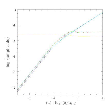
FIG. 1.: We present the evolutions of the adiabatic density perturbations in the corresponding comoving gauges $\delta_{(i)v_{(i)}}$ for several components. $(i)$ includes the baryon (dot, black), CDM (dot-long dash, blue), photon (long dash, red), massless neutrino (short-dash, green), and massive neutrino (solid, cyan). The two figures are (a) $k/a_{0}=0.1Mpc^{-1}$ and (b) $k/a_{0}=0.01Mpc^{-1}$. Also presented is the $\varphi_{v}$ (dot-short dash, yellow) where $v$ is the collective fluid velocity. The parameters are: $h=0.65$, $\Omega_{b0}=0.06$, $\Omega_{C0}=0.5$, $\Omega_{\gamma 0}=5.85\times 10^{-5}$, $\Omega_{\nu 0}=3.99\times 10^{-5}$, and $\Omega_{\nu_{m}0}=0.44$. We consider a flat background with vanishing $\Lambda$. The absolute value of the vertical scale is arbitrary.

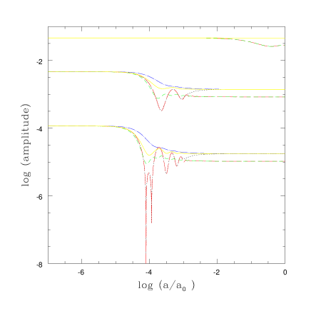
FIG. 2.: We present the evolutions of $\varphi$ in various comoving gauge conditions based on fixing the velocity variables of the components, i.e., $\varphi_{v_{(i)}}$, and $\varphi_{v}$: the baryon $\varphi_{v_{(b)}}$ (dot, black), the CDM $\varphi_{v_{(C)}}$ (dot-long dash, blue), the photon $\varphi_{v_{(\gamma)}}$ (long dash, red), the massless neutrino $\varphi_{v_{(\nu)}}$ (short dash, green), and the one based on the collective velocity $\varphi_{v}$ (dot-short dash, yellow). We consider three different scales: $k/a_{0}=0.001$ (top), $0.1$ and $0.2Mpc^{-1}$ (bottom). For $k/a_{0}=0.001Mpc^{-1}$, the baryon, CDM, and the collective one are overlapped (top), and the photon and massless neutrino are overlapped (bottom). In order to present the behaviors in three scales in one frame, we change the absolute scale of the amplitude arbitrarily. The parameters are: $\Omega_{C0}=0.94$, $\Omega_{\nu_{m}0}=0$, and the other parameters are the same as in Fig. 1.

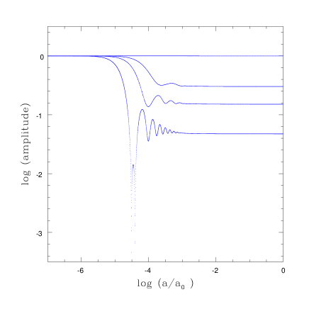
FIG. 3.: The evolution of $\varphi_{v}$ for different scales: $k/a_{0}=0.0001$ (top), $0.001$, $0.01$, $0.2$, and $0.5Mpc^{-1}$ (bottom). The cases of $k/a_{0}=0.0001$ and $0.001Mpc^{-1}$ are almost overlapped. The parameters are the same as in Figure 2.

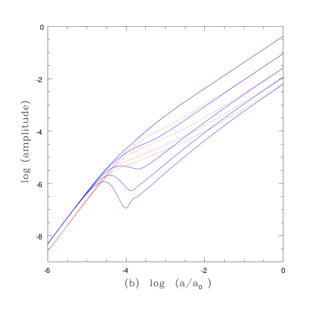
FIG. 4.: We present the evolution of density perturbation in the comoving gauge of the massive neutrino, $\delta_{(\nu_{m})v_{(\nu_{m})}}$, for different scales: $k/a_{0}=0.01$ (top), $0.1$, $0.2$, $0.3$ and $0.4Mpc^{-1}$ (bottom). Figure (a) considers the massive neutrino dominated model with a parameter $\Omega_{\nu_{m}0}=0.94$. Figure (b) considers substantial amount of the CDM with parameters $\Omega_{C0}=0.5$ and $\Omega_{\nu_{m}0}=0.44$. In Figure (b) we show the evolution of CDM $\delta_{(C)v_{(C)}}$ (dotted, red) as well. The other parameters are the same as in Fig. 2.

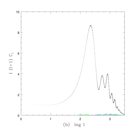
FIG. 5.: We present the power spectra $\ell(\ell+1)C_{\ell}$ of the scalar-type perturbation: the temperature $C_{\ell}^{\Theta\Theta}$ (top, black), the polarization $C_{\ell}^{EE}$ (middle, green), and the cross correlation $C_{\ell}^{\Theta E}$ (bottom, blue). We take the adiabatic initial condition with the scale-invariant ($n_{S}=1$) spectrum. Figure (a) shows the spectra in logarithmic scale, and (b) shows in real scale. We normalize the spectra using $\ell(\ell+1)C_{\ell}^{\Theta\Theta}=1$ for $\ell=10$. The parameters are: $\Omega_{C0}=0.25$, $\Omega_{\Lambda 0}=0.69$, $\Omega_{\nu_{m}0}=0.$, and the other parameters are the same as in Fig. 1.

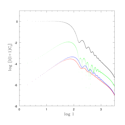
FIG. 6.: We present the power spectra $\ell(\ell+1)C_{\ell}$ of the gravitational wave: the temperature $C_{\ell}^{\Theta\Theta}$ (top, black), the cross correlation $C_{\ell}^{\Theta E}$ (green), and the polarizations $C_{\ell}^{EE}$ (blue) and $C_{\ell}^{BB}$ (bottom, red). As the initial condition we take the scale-invariant ($n_{T}=0$) spectrum and the solution with constant amplitude. We normalize the spectra using $\ell(\ell+1)C_{\ell}^{\Theta\Theta}=1$ for $\ell=10$. The parameters are the same as in Figure 5.

REFERENCES

- [1] P. de Bernardis, et al., Nature 404, 955 (2000); C. B. Netterfield, et al., astro-ph/0104460.
- [2] S. Hanany, et al., Astrophys. J. 545, L5 (2000); A. T. Lee, et al., astro-ph/0104459.
- [3] A. A. Penzias and R. W. Wilson, Astrophys. J. 142, 419 (1965).
- [4] R. K. Sachs and A. M. Wolfe, Astrophys. J. 147, 73 (1967).
- [5] P. J. E. Peebles and J. T. Yu, Astrophys. J. 162, 815 (1970).
- [6] E. M. Lifshitz, J. Phys. (USSR) 10, 116 (1946); E. M. Lifshitz and I. M. Khalatnikov, Adv. Phys. 12, 185 (1963).
- [7] E. R. Harrison, Rev. Mod. Phys. 39, 862 (1967).
- [8] H. Nariai, Prog. Theor. Phys. 41, 686 (1969).
- [9] J. M. Bardeen, Phys. Rev. D 22, 1882 (1980).
- [10] V. N. Lukash, Sov. Phys. JETP Lett. 31, 596 (1980); Sov. Phys. JETP 52, 807 (1980).
- [11] E. Gliner, Sov. Phys. JETP 22, 378 (1966); D. Kazanas, Astrophys. J. 241, L59 (1980); A. A. Starobinsky, Phys. Lett. B 91, 99 (1980); A. H. Guth, Phys. Rev. D 23, 347 (1981).
- [12] J. M. Bardeen, in Cosmology and Particle Physics, edited by L. Fang and A. Zee (Gordon and Breach, London, 1988), p. 1.
- [13] J. Hwang, Astrophys. J. 375, 443 (1991).
- [14] D. S. Salopek, J. R. Bond, and J. M. Bardeen, Phys. Rev. D 40, 1753 (1989).
- [15] J. Hwang, Class. Quant. Grav. 7, 1613 (1990).
- [16] J. Ehlers, Gen. Rel. Grav. 25, 1225 (1993), translated from German originally published in Akad. Wiss. Lit. Mainz, Abhandl. Math.-Nat. Kl. 11 792 (1961); G. F. R. Ellis, in General relativity and cosmology, Proceedings of the international summer school of physics Enrico Fermi course 47, edited by R. K. Sachs (Academic Press, New York, 1971), 104; G. F. R. Ellis, in Cargese Lectures in Physics, edited by E. Schatzmann (Gorden and Breach, New York, 1973), 1.
- [17] H. Kodama and M. Sasaki, Prog. Theor. Phys. Suppl. 78, 1 (1984).
- [18] J. Hwang, Astrophys. J. 415, 486 (1993).
- [19] J. Hwang, Astrophys. J. 427, 542 (1994).
- [20] J. Hwang and H. Noh, Phys. Rev. D 54, 1460 (1996).
- [21] J. M. Stewart and M. Walker, Prog. R. Soc. Lond. A 341, 49 (1974).
- [22] G. F. R. Ellis and M. Bruni, Phys. Rev. D 40, 1804 (1989).
- [23] H. Noh. and J. Hwang, Phys. Letts. B in press, astro-ph/0107069.
- [24] R. W. Lindquist, Ann. Phys. 37, 487 (1966); J. Ehlers, in General relativity and cosmology, Proceedings of the international summer school of physics Enrico Fermi course 47, edited by R. K. Sachs (Academic Press, New York, 1971), 1; J. M. Stewart, Non-Equilibrium Relativistic Kinetic Theory, Lecture Notes in Physics Vol. 10 (Springer-Verlag, New York, 1971).
- [25] A. V. Zakharov, Sov. Phys. J. 21, 289 (1978); H. Kodama and M. Sasaki, Internat. J. Mod. Phys. A 1, 265 (1986); M. Kasai and K. Tomita, Phys. Rev. D 33, 1576 (1986).
- [26] P. J. E. Peebles, Astrophys. J. 258, 415 (1982).
- [27] J. R. Bond and A. S. Szalay, Astrophys. J. 274, 443 (1983).
- [28] W. Hu, U. Seljak, M. White, and M. Zaldarriaga, Phys. Rev. D 57, 3290 (1998).
- [29] M. Zaldarriaga and U. Seljak, Phys. Rev. D 55, 1830 (1997).
- [30] E. Newman and R. Penrose, J. Math. Phys. 7, 863 (1966).
- [31] G. Dautcourt and K. Rose, Astron. Nachr. 299, 13 (1978).
- [32] D. H. Lyth and A. Woszczyna, Phys. Rev. D 52, 3338 (1995).
- [33] W. Hu and M. White, Phys. Rev. D 56, 596 (1997).
- [34] G. Dautcourt, Physica Scripta 21, 714 (1980).
- [35] J. R. Bond and G. Efstathiou, Astrophys. J. 285, L45 (1984).
- [36] M. Kamionkowski, A. Kosowsky, and A. Stebbins, Phys. Rev. Lett. 78, 2058 (1997); U. Seljak and M. Zaldarriaga, ib id 78, 2054 (1997).
- [37] A. Kosowsky, Annals of Phys. 246, 49 (1996); A. Challinor, Phys. Rev. D 62, 043004 (2000).
- [38] A. Lewis, A. Challinor and N. Turok, astro-ph/0106536.
- [39] C. Ma and E. Bertschinger, Astrophys. J. 455, 7 (1995).
- [40] J. R. Bond, in Cosmology and Large Scale Structure, edited by R. Schaeffer, J. Silk, M. Spiro, and J. Zinn-Justin (Elsevier Science, Amsterdam, 1996), 469.
- [41] P. T. P. Viana and A. R. Liddle, Phys. Rev. D 57, 674 (1998).
- [42] A. Lewis, A. Challinor, and A. Lasenby, Astrophys. J. 538, 473 (2000).
- [43] S. Seager, D. D. Sasselov, and D. Scott, Astrophys. J. 523, 1 (1999).
- [44] M. Bucher, K. Moodley, and N. Turok, Phys. Rev. D 62, 083508 (2000).
- [45] S. Dodelson, E. Gates, and A. Stebbins, Astrophys. J. 467, 10 (1996).
- [46] J. M. Stewart, Astrophys. J. 176, 323 (1972); P. J. E. Peebles, ib id 180, 1 (1973); A. Rebhan, ib id 391, 385 (1992); A. Rebhan and D. J. Schwarz, Phys. Rev. D 50, 2541 (1994).
- [47] A. V. Zakharov, Sov. Phys. J. 21, 295 (1978); Sov. Phys. J. 21, 442 (1978); Sov. Astron. 22, 528 (1978); Sov. Phys. JETP 50, 221 (1979); Sov. Astron. 26, 265 (1982); E. T. Vishniac, Astrophys. J. 257, 456 (1982); A. V. Zakharov, Sov. Phys. JETP 69, 437 (1989); Sov. Astron. 33, 624 (1989).
- [48] R. Durrer, Astro. Astrophys. 208, 1 (1989).
- [49] I. H. Gilbert, Astrophys. J. 144, 233 (1965).
- [50] A. G. Doroshkevich, Ya. B. Zel’dovich, and R. A. Sunyaev, Sov. Astron. 22, 523 (1978).
- [51] J. R. Bond and G. Efstathiou, Mon. Not. R. Astron. Soc. 226, 655 (1987).
- [52] P. J. E. Peebles, The large-scale structure of the universe (Princeton Univ. Press, Princeton, 1980); J. Silk and M. L. Wilson, Physica Scripta 21, 708 (1980); M. L. Wilson and J. Silk, Astrophys. J. 243, 14 (1981); M. L. Wilson, ib id 273, 2 (1983); G. Efstathiou and J. R. Bond, Mon. Not. R. Astron. Soc. 218, 103 (1986); N. Gouda and M. Sasaki, Prog. Theor. Phys. 76, 1016 (1986); G. Efstathiou and J. R. Bond, Mon. Not. R. Astron. Soc. 227, 33 (1987); N. Gouda, M. Sasaki, and Y. Suto, Astrophys. J. 341, 557 (1989); N. Sugiyama, Prog. Theor. Phys. 81, 1021 (1989); N. Gouda, N. Sugiyama, and M. Sasaki, ib id 85, 1023 (1991); N. Sugiyama and N. Gouda, ib id 88, 803 (1992).
- [53] U. Seljak, Astrophys. J. 435, L87 (1994); W. Hu and N. Sugiyama, Phys. Rev. D 51, 2599 (1995); Astrophys. J. 444, 489 (1995); ib id 471, 542 (1996).
- [54] R. K. Schaefer and A. A. de Laix, Astrophys. J. Suppl. 105, 1 (1996).
- [55] T. Gebbie and G. F. R. Ellis, astro-ph/9804316; R. Maartens, T. Gebbie and G. Ellis, Phys. Rev. D 59, 083506 (1999); T. Gebbie, P. Dunsby, and G. Ellis, Ann. Phys. (N.Y.) 282, 321 (2000); A. Challinor, Gen. Rel. Grav. 32, 1059 (2000); Class. Quant. Grav. 17, 871 (2000);
- [56] U. Seljak and M. Zaldarriaga, Astrophy. J. 469, 437 (1996); M. Zaldarriaga and U. Seljak, Astrophy. J. Suppl. 129, 431 (2000).
- [57] J. R. Bond, G. Efstathiou, and M. Tegmark, Mon. Not. R. Astron. Soc. 291, L33 (1997).
- [58] A. D. Sakharov, Sov. Phys. JETP 22, 241 (1966).
- [59] R. A. Sunyaev and Ya. B. Zel’dovich, Astrophys. Space Sci. 7, 3 (1970).
- [60] Ya. B. Zel’dovich and I. D. Novikov, Relativistic astrophysics, Vol 2, The structure and evolution of the universe (Univ. Chicago Press, Chicago, 1983).
- [61] A. Albrecht, astro-ph/9612015.
- [62] R. H. Dicke, Phys. Rev. 125, 2163 (1962); B. Whitt, Phys. Lett. B 145, 176 (1984); G. Magnano and L. M. Sokołowski, Phys. Rev. D 50, 5039 (1994); V. Faraoni, E. Gunzig, and P. Nardone, Fundamentals of Cosmic Physics, 20, 121 (1999).
- [63] J. Hwang, Class. Quant. Grav. 14, 1981 (1997).
- [64] S. W. Hawking, Astrophys. J., 145, 544 (1966).
- [65] J. Hwang and E. T. Vishniac, Astrophys. J., 353, 1 (1990).
- [66] R. Arnowitt, S. Deser, and C. W. Misner, in Gravitation: an introduction to current research, edited by L. Witten (Wiley, New York, 1962), p. 227.
- [67] W. Israel, Ann. Phys. 100, 310 (1976).