Cosmological Perturbations
in an
Inflationary Universe

Abstract

After introducing the perturbed metric tensor in a Friedmann-Robertson–Walker (FRW) background we review how the metric perturbations can be split into scalar, vector and tensor perturbations according to their transformation properties on spatial hypersurfaces and how these perturbations transform under small coordinate transformations. This allows us to introduce the notion of gauge-invariant perturbations and to provide their governing equations. We then proceed to give the energy- and momentum-conservation equations and Einstein’s field equations for a perturbed FRW metric for a single fluid and extend this set of equations to the multi-fluid case including energy transfer. In particular we are able to give an improved set of governing equations in terms of newly defined variables in the multi-fluid case. We also give the Klein-Gordon equations for multiple scalar fields. After introducing the notion of adiabatic and entropic perturbations we describe under what conditions curvature perturbations are conserved on large scales. We derive the “conservation law” for the curvature perturbation for the first time using only the energy conservation equation [105].

We then investigate the dynamics of assisted inflation. In this model an arbitrary number of scalar fields with exponential potentials evolve towards an inflationary scaling solution, even if each of the individual potentials is too steep to support inflation on its own. By choosing an appropriate rotation in field space we can write down for the first time explicitly the potential for the weighted mean field along the scaling solution and for fields orthogonal to it. This allows us to present analytic solutions describing homogeneous and inhomogeneous perturbations about the attractor solution without resorting to slow-roll approximations. We discuss the curvature and isocurvature perturbation spectra produced from vacuum fluctuations during assisted inflation [79].

Finally we investigate the recent claim that preheating after inflation may affect the amplitude of curvature perturbations on large scales, undermining the usual inflationary prediction. We analyze the simplest model of preheating analytically, and show that in linear perturbation theory the effect is negligible. The dominant effect is second-order in the field perturbation and we are able to show that this too is negligible, and hence conclude that preheating has no significant influence on large-scale perturbations in this model. We briefly discuss the likelihood of an effect in other models [62].

We end this work with some concluding remarks, possible extensions and an outlook to future work.

To my parents.

I would like to thank my supervisor David Wands for his kind guidance and his patience and express my gratitude to David Matravers and Roy Maartens.

I must also like to thank the Relativity and Cosmology Group for their constant inspiration and the School of Computer Science and Mathematics and the University of Portsmouth for funding this work.

1 Introduction

It has almost become impossible to write about cosmology without having at least mentioned once that we are now experiencing and living through “the golden age” of cosmology. This thesis is no exception.

The standard inflationary paradigm is an extremely successful model in explaining observed structures in the Universe (see Refs. [60, 61, 75] for reviews). In this cosmological model the universe is dominated at early times by a scalar field that gives rise to a period of accelerated expansion, which has become known as inflation. Inhomogeneities originate from the vacuum fluctuations of the inflaton field, which on being stretched to large scales become classical perturbations. The field inhomogeneities generate a perturbation in the curvature of uniform density hypersurfaces, and later on these inhomogeneities are inherited by matter and radiation when the inflaton field decays. Large scale structure then forms in the eras of radiation and matter domination through gravitational attraction of the seed fluctuations.

Defect models of cosmic structure formation have for a long period been the only viable competitor for the inflation based models. In these models a network of defects, usually cosmic strings, seeds the growth of cosmic structure continuously through the history of the Universe. Unfortunately, at least for the researchers involved in the investigation of these models, recent cosmic microwave background (CMB) observations have nearly ruled these models out [1].

The amount of data available in cosmology is increasing rapidly. New galaxy surveys, like the 2-degree-Field and the Sloan-Digital-Sky-Survey are beginning to determine the matter power spectrum, the distribution of galaxies and clusters of galaxies, on large scales. New balloon based experiments, like Boomerang and Maxima, have already measured the fluctuations in the CMB with unprecedented accuracy. Forthcoming satellite missions, like MAP and Planck, are going to improve these results even more.

Although it might seem that extending the parameter space of the cosmological models that are investigated will lead to a decrease in accuracy, the quality and sheer quantity of the new data will nevertheless allow us to constrain the parameter space enough to rule out large classes of models and to give hints in which direction we should direct our theoretical and experimental attention in future [13]. The combination of data from different CMB experiments with large scale structure and super-nova observations will be particularly useful in this respect.

But to take full advantage from these new experiments and the new data they will provide one has to make accurate theoretical predictions. In this work we extend the theory of cosmological perturbations. We apply the methods we have developed to investigate some models of the early universe and calculate their observable consequences.

The evolution and the dynamics of the universe are governed by Einstein’s theory of relativity, whose field equations are [82]

$$G_{\mu\nu}=8\pi G~{}T_{\mu\nu}\,,$$ (1.1)

where $G_{\mu\nu}$ is the Einstein tensor, $G$ Newton’s constant and $T_{\mu\nu}$ the energy-momentum tensor. From the contracted Bianchi identity $G_{\mu\nu;}^{~{}~{}~{}\nu}=0$, we find that the energy-momentum tensor is covariantly conserved,

$$T_{\mu\nu;}^{~{}~{}~{}\nu}=0\,.$$ (1.2)

In an unperturbed Friedmann-Robertson-Walker (FRW) universe, described by the line element

$$ds^{2}=-dt^{2}+a^{2}(t)\left[\frac{dr^{2}}{1-\kappa r^{2}}+r^{2}\left(d\theta^{2}+\sin^{2}\theta d\phi^{2}\right)\right]\,,$$ (1.3)

the homogeneous spatial hypersurfaces pick out a natural cosmic time coordinate, $t$, and hence a (3+1) decomposition of spacetime. Here $a(t)$ is the scale factor and $r$, $\theta$ and $\phi$ are polar coordinates. But in the presence of inhomogeneities this choice of coordinates is no longer unambiguous.

The need to clarify these ambiguities lead to the fluid-flow approach which uses the velocity field of the matter to define perturbed quantities orthogonal to the fluid-flow [38, 72, 74, 76, 24, 11]. An alternative school has sought to define gauge-invariant perturbations in any coordinate system by constructing quantities that are explicitly invariant under first-order coordinate transformations [2, 55, 84, 23, 8]. Results obtained in the two formalisms can be difficult to compare. One stresses the virtue of invariance of metric perturbations under gauge transformations, while the other claims to be covariant and therefore manifestly gauge-invariant due to its physically transparent definition.

We put special emphasis on the fact that perturbations defined on an unambiguous physical choice of hypersurface can always be written in a gauge-invariant manner. In the coordinate based formalism [2] the choice of hypersurface implies a particular choice of temporal gauge. By including the spatial gauge transformation from an arbitrary initial coordinate system all the metric perturbations can be given in an explicitly gauge-invariant form. In this language, linear perturbations in the fluid-flow or “covariant” approach appear as a particular gauge choice (the comoving orthogonal gauge [2, 55]) whose metric perturbations can be given in an explicitly gauge-invariant form. But there are many other possible choices of hypersurface, including the zero-shear (or longitudinal or conformal Newtonian) gauge [2, 55, 84, 77] in which gauge-invariant quantities may be defined.

Whereas there are still more things we do not know than we do know, and even more things we don’t even know we don’t know, it is safe to say that the age of “golden-ish” cosmology has begun.

2 Cosmological Perturbation Theory

In this section we present the fundamental building blocks of perturbation theory in a cosmological context. After introducing the concept of gauge and gauge transformation we give the governing equations in gauge dependent and gauge invariant form for scalar, vector and tensor quantities in a perturbed Friedmann-Robertson-Walker (FRW) spacetime in the single fluid case. After a short section on scalar fields we then give the governing equations for multiple fluids. We conclude this section with an application of the theory to quantities that are conserved on large scales.

2.1 Decomposing the metric tensor

We consider first-order perturbations about a FRW background, so that the metric tensor can be split up as

$$g_{\mu\nu}=g^{(0)}_{\mu\nu}+\delta g_{\mu\nu}\,,$$ (2.4)

where the background metric $g^{(0)}_{\mu\nu}$ is given by

$$g^{(0)}_{\mu\nu}=a^{2}(\eta)\left(\begin{array}[]{cc}-1&0\\ 0&\gamma_{ij}\end{array}\right)\,,$$ (2.5)

and $\gamma_{ij}$ is the metric on the 3-dimensional space with constant curvature $\kappa$. We will denote covariant spatial derivatives on this space as $X_{abc\ldots|i}$ .

The metric tensor has 10 independent components in 4 dimensions. For linear perturbations it turns out to be very useful to split the metric perturbation into different parts labelled scalar, vector or tensor according to their transformation properties on spatial hypersurfaces [2, 96]. The reason for splitting the metric perturbation into these three types is that they are decoupled in the linear perturbation equations.
Scalar perturbations can always be constructed from a scalar quantity, or its derivatives, and any background quantities such as the 3-metric $\gamma_{ij}$. We can construct any first-order scalar metric perturbation in terms of four scalars $\phi$, $B$, $\psi$ and $E$, where

$$\delta g_{00} = -a^{2}2\phi\,,$$ (2.6)

$$\delta g_{0i} = \delta g_{i0}=a^{2}B_{|i}\,,$$ (2.7)

$$\delta g_{ij} = -2a^{2}(\psi\;\gamma_{ij}-E_{|ij})\,.$$ (2.8)

Any 3-vector, such as $B_{|i}$, constructed from a scalar is necessarily curl-free, i.e., $B_{|[ij]}=0$. Thus one can distinguish an intrinsically vector part of the metric perturbation $\delta g_{0i}$, which we denote by $-S_{i}$, which gives a non-vanishing $\delta g_{0[i|j]}$. Similarly we can define a vector contribution to $\delta g_{ij}$ constructed from the (symmetric) derivative of a vector $F_{(i|j)}$. The scalar perturbations are distinguished from the vector contribution by requiring that the vector part is divergence-free, i.e., $\gamma^{ij}S_{i|j}=0$. This means that there can be no contribution to $\delta g_{00}$ from vector perturbations to first-order. The decomposition of a vector field into curl- and divergence-free parts in Euclidean space is known as Helmholtz’s theorem. The curl-free and divergence-free parts are also called longitudinal and solenoidal, respectively.

Finally there is a tensor contribution to $\delta g_{ij}=a^{2}h_{ij}$ which is transverse ($\gamma^{jk}h_{ij|k}=0$), i.e., divergence-free, and trace-free ($\gamma^{ij}h_{ij}=0$) which cannot be constructed from scalar or vector perturbations.

We have introduced four scalar functions, two (spatial) vector valued functions with three components each, and a symmetric spatial tensor with six components. But these functions are subject to several constraints: $h_{ij}$ is transverse and traceless, which contributes four constraints, $F_{i}$ and $S_{i}$ are divergence-free, one constraint each. We are therefore finally left 10 new degrees of freedom, the same number as the independent components of the perturbed metric.

We can now write the most general metric perturbation to first-order as

$$\delta g_{\mu\nu}=a^{2}(\eta)\left(\begin{array}[]{cc}-2\phi&B_{|i}-S_{i}\\ B_{|j}-S_{j}&-2\psi\gamma_{ij}+2E_{|ij}+F_{i|j}+F_{j|i}+h_{ij}\end{array}\right)\,.$$

The contravariant metric tensor, including the perturbed part, follows by requiring (to first order), $g_{\mu\nu}~{}g^{\nu\lambda}=\delta_{\mu}^{~{}\lambda}$, which gives

$$g^{\mu\nu}=a^{-2}(\eta)\left(\begin{array}[]{cc}-(1-2\phi)&B_{|}^{~{}i}-S^{i}\\ B_{|}^{~{}j}-S^{j}&(1+2\psi)\gamma^{ij}-2E_{|}^{~{}ij}-F^{i~{}j}_{~{}|}-F^{j~{}i}_{~{}|}-h^{ij}\end{array}\right)\,.$$

Thus we have the general linearly perturbed line element:

$$ds^{2}= a^{2}(\eta) \left\{-(1+2\phi)d\eta^{2}+2(B_{|i}-S_{i})d\eta dx^{i}\right.$$ (2.9)

$$\left.+\left[(1-2\psi)\gamma_{ij}+2E_{|ij}+2F_{i|j}+h_{ij}\right]dx^{i}dx^{j}\right\}\,.$$

2.2 Coordinate Transformation

We use Eq. (2.9) as a starting point and perform a small coordinate transformation, where the new coordinate system is denoted by a tilde.

The homogeneity of a FRW spacetime gives a natural choice of coordinates in the absence of perturbations. But in the presence of first-order perturbations we are free to make a first-order change in the coordinates, i.e., a gauge transformation,

$$\tilde{\eta}=\eta+\xi^{0}\,,\qquad\tilde{x}^{i}=x^{i}+\xi_{|}^{~{}i}+\bar{\xi}^{i}\,,$$ (2.10)

where $\xi^{0}=\xi^{0}(\eta,x^{i})$ and $\xi=\xi(\eta,x^{i})$ are arbitrary scalar functions, and $\bar{\xi}^{i}=\bar{\xi}^{i}(\eta,x^{i})$ is a divergence-free 3-vector. The function $\xi^{0}$ determines the choice of constant-$\eta$ hypersurfaces, that is the time-slicing, while $\xi_{|}^{~{}i}$ and $\bar{\xi}^{i}$ then select the spatial coordinates within these hypersurfaces. The choice of coordinates is arbitrary to first-order and the definitions of the first-order metric and matter perturbations are thus gauge-dependent.

The result of the transformation Eq. (2.10) acting on any quantity is that of taking the Lie derivative of the background value of that quantity, i.e. for every tensor $T$ one has [101]

$$\tilde{\delta T}=\delta T+{\cal{L}}_{\xi}T_{0}\,,$$ (2.11)

where $T_{0}$ is the background value of that quantity.

We use a slightly different approach by directly perturbing the line element in Eq. (2.9). Starting with the total differentials of $\xi^{0}$ and $\xi$ and $d\bar{\xi}^{i}$

$$d\xi^{0} = {\xi^{0}}^{\prime}d\tilde{\eta}+\xi^{0}_{~{}|i}d\tilde{x}^{i}\,,$$ (2.12)

$$d\xi = \xi^{\prime}d\tilde{\eta}+\xi_{~{}|j}d\tilde{x}^{j}\,,$$ (2.13)

$$d\bar{\xi}^{i} = \bar{\xi}^{i\prime}d\tilde{\eta}+\bar{\xi}^{i}_{~{}|j}d\tilde{x}^{j}\,,$$ (2.14)

we get using Eq. (2.10)

$$d\eta = d\tilde{\eta}-{\xi^{0}}^{\prime}d\tilde{\eta}-\xi^{0}_{~{}|i}d\tilde{x}^{i}\,,$$

$$dx^{i} = d\tilde{x}^{i}-(\xi^{\prime~{}i}_{|}+\bar{\xi}^{i\prime})d\tilde{\eta}-(\xi^{~{}i}_{|~{}j}+\bar{\xi}^{i}_{~{}|j})d\tilde{x}^{j}\,,$$ (2.15)

where we have used the fact that $\xi^{0}(\eta,x^{i})=\xi^{0}(\tilde{\eta},\tilde{x}^{i})$ and $\xi(\eta,x^{i})=\xi(\tilde{\eta},\tilde{x}^{i})$, to first order in the coordinate transformations.
Substituting the differentials Eq. (2.15) into Eq. (2.9) and using

$$a(\eta)=a(\tilde{\eta})-\xi^{0}a^{\prime}(\tilde{\eta})\,,$$ (2.16)

we then get for the line element in the “new” coordinate system, working only to first order in both the metric perturbations and the coordinate transformations:

$$ds^{2} = a^{2}\left(\tilde{\eta}\right)\left\{-\left(1+2\left(\phi-h\xi^{0}-\xi^{0\prime}\right)\right)d{\tilde{\eta}}^{2}+2\left(B+\xi^{0}-\xi^{\prime}\right)_{|i}d\tilde{\eta}d\tilde{x}^{i}\right.$$ (2.17)

$$\left.-2\left(S_{i}+\bar{\xi}^{\prime}_{i}\right)d\tilde{\eta}d\tilde{x}^{i}+\left[\left(1-2\left(\psi+h\xi^{0}\right)\right)\gamma_{ij}+2\left(E-\xi\right)_{|ij}\right.\right.$$

$$\left.\left.+2\left(F_{i|j}-\bar{\xi}_{i|j}\right)+h_{ij}\right]d\tilde{x}^{i}d\tilde{x}^{j}\right\}\,.$$

The general form of the line element presented in Eq. (2.9) must be invariant under infinitesimal coordinate transformations, since the line element $ds^{2}$ is a scalar invariant. We can read off the transformation equations for the metric perturbations by writing down the line element in the “new” coordinate system

$$ds^{2}= a^{2}(\tilde{\eta}) \left\{-(1+2\tilde{\phi})d\tilde{\eta}^{2}+2(\tilde{B}_{|i}-\tilde{S}_{i})d\tilde{\eta}d\tilde{x}^{i}\right.$$ (2.18)

$$\left.+\left[(1-2\tilde{\psi})\gamma_{ij}+2\tilde{E}_{|ij}+2\tilde{F}_{i|j}+\tilde{h}_{ij}\right]d\tilde{x}^{i}d\tilde{x}^{j}\right\}\,.$$

The coordinate transformation of Eq. (2.10) induces a change in the scalar functions $\phi$, $\psi$, $B$ and $E$ defined by Eq. (2.9)

$$\tilde{\phi} = \phi-h\xi^{0}-\xi^{0\prime}\,,$$ (2.19)

$$\tilde{\psi} = \psi+h\xi^{0}\,,$$ (2.20)

$$\tilde{B} = B+\xi^{0}-\xi^{\prime}\,,$$ (2.21)

$$\tilde{E} = E-\xi\,,$$ (2.22)

where $h=a^{\prime}/a$ and a dash indicates differentiation with respect to conformal time $\eta$. The vector valued functions $S_{i}$ and $F_{i}$ transform as

$$\tilde{F}_{i} = F_{i}-\bar{\xi}_{i},$$ (2.23)

$$\tilde{S}_{i} = S_{i}+\bar{\xi}_{i}^{\prime}.$$ (2.24)

The tensor part of the perturbation, $h_{ij}$, is unaffected by the gauge transformations.

2.3 Time slicing and spatial hypersurfaces

We now relate the metric perturbations to physical, that is observable, quantities [55]. The unit time-like vector field orthogonal to constant-$\eta$ hypersurfaces is

$$N^{\mu}={1\over a}(1-\phi,-B_{|}^{~{}i}+S^{i})\,,$$ (2.25)

and the covariant vector field is

$$N_{\mu}=-a(1+\phi,0)\,.$$ (2.26)

The covariant derivative of the time like unit vector field $N_{\mu}$ can be decomposed uniquely as follows [101] :

$$N_{\mu;\nu}=\sigma_{\mu\nu}+\frac{1}{3}\theta P_{\mu\nu}-a_{\mu}N_{\nu}\,,$$ (2.27)

where the projection tensor $P_{\mu\nu}$ is given by

$$P_{\mu\nu}=g_{\mu\nu}+N_{\mu}N_{\nu}.$$ (2.28)

The expansion rate is given as

$$\theta=N^{\mu}_{~{};\mu}\,,$$ (2.29)

the shear is

$$\sigma_{\mu\nu}=\frac{1}{2}P^{~{}\alpha}_{\mu}P^{~{}\beta}_{\nu}\left(N_{\alpha;\beta}+N_{\beta;\alpha}\right)-\frac{1}{3}\theta P_{\mu\nu}\,,$$ (2.30)

and the acceleration is

$$a_{\mu}=N_{\mu;\nu}N^{\nu}\,.$$ (2.31)

Note that on spatial hypersurfaces the vorticity, the shear, the acceleration and the expansion coincide with their Newtonian counterparts in fluid dynamics [81, 39].

The extrinsic curvature of hypersurfaces defined by $N_{\mu}$ is defined as

$$K_{\mu\nu}=-P_{\nu}^{~{}\lambda}N_{\mu;\nu}\,.$$ (2.32)

The Raychauduri equation [39] is given solely in terms of geometric quantities and gives the evolution of the expansion $\theta$ with respect to proper time as

$$\frac{d\theta}{d\tau}=a^{\mu}_{~{};\mu}-\sigma_{\mu\nu}\sigma^{\mu\nu}-\frac{1}{3}\theta^{2}-R_{\mu\nu}N^{\mu}N^{\nu}\,.$$ (2.33)

We can write the expansion, acceleration and shear of the vector field for a perturbed FRW spacetime, considering scalar quantities first, as

$$\theta = 3{a^{\prime}\over a^{2}}\left(1-\phi\right)-{3\over a}\psi^{\prime}-{1\over a}\nabla^{2}\left(B-E^{\prime}\right)\,,$$ (2.34)

$$a_{i} = \phi_{|i}\,,$$ (2.35)

$$\sigma_{ij} = a\left(\sigma_{|ij}-{1\over 3}\gamma_{ij}\nabla^{2}\sigma\right)\,,$$ (2.36)

where the scalar describing the shear is

$$\sigma=-B+E^{\prime}\,,$$ (2.37)

and where the time components are zero, i.e. $a_{0}=0$, $\sigma_{0\mu}=0$. Note that for an unperturbed background the expansion $\theta$ coincides with the expansion rate of the spatial volume per unit proper time.

The intrinsic spatial curvature on hypersurfaces of constant conformal time $\eta$ is given by [2, 55]

$${}^{(3)}R={6\kappa\over a^{2}}+\frac{12\kappa}{a^{2}}\psi+\frac{4}{a^{2}}\nabla^{2}\psi\,.$$ (2.38)

For a perturbation with comoving wavenumber $k$, such that $\nabla^{2}\psi=-k^{2}\psi$, we therefore have

$$\delta^{(3)}R=\frac{4}{a^{2}}\left(3\kappa-k^{2}\right)~{}\psi\,,$$ (2.39)

and $\psi$ is often simply referred to as the curvature perturbation.

For vector perturbations we find $\bar{a}_{\mu}=0$, $\bar{\sigma}_{00}=\bar{\sigma}_{0j}=0$, and $\bar{\theta}=0$, and the only non-zero first order quantity is the shear given by

$$\tau_{ij}\equiv\bar{\sigma}_{ij}=\frac{1}{2}a\left\{\left(S_{i|j}+S_{j|i}\right)+\left(F_{i|j}+F_{j|i}\right)^{\prime}\right\}\,,$$ (2.40)

where we distinguished the vector quantities from the scalar ones by a “bar”.

There is no tensor contribution to the expansion, the acceleration and the vorticity, but there is a non-zero contribution of the tensor pertubations to the shear,

$${}^{\rm{(tensor)}}\sigma_{ij}=\frac{1}{2}a\,h^{\prime}_{ij}\,.$$ (2.41)

2.3.1 Evolution of the curvature perturbation

We can now give a simple expression for the evolution of the curvature perturbation $\psi$. Multiplying Eq. (2.34) through by $(1+\phi)$ in order to give the expansion with respect to coordinate time, $t\equiv\int ad\eta$, we get

$$\tilde{\theta}=(1+\phi)\theta=3H-3\dot{\psi}+\nabla^{2}\tilde{\sigma}\,,$$ (2.42)

where $\tilde{\sigma}\equiv\dot{E}-B/a$. We can write this as an equation for the time evolution of $\psi$ in terms of the perturbed expansion, $\delta\tilde{\theta}\equiv\tilde{\theta}-3H$, and the shear:

$$\dot{\psi}=-{1\over 3}\delta\tilde{\theta}+{1\over 3}\nabla^{2}\tilde{\sigma}\,.$$ (2.43)

Note that this is independent of the field equations and follows simply from the geometry. It shows that on large scales ($\nabla^{2}\tilde{\sigma}\to 0$) the change in the curvature perturbation, $\dot{\psi}$, is proportional to the change in the expansion $\delta\tilde{\theta}$.

2.4 The stress-energy tensor for a fluid,
including anisotropic stress

Thus far we have concerned ourselves solely with the metric and its representation under different choices of coordinates. However, in any non-vacuum spacetime we will also have matter fields to consider. Like the metric, the coordinate representation of these fields will also be gauge-dependent.

The stress-energy tensor of a fluid with density $\rho$, isotropic pressure $p$ and 4-velocity $u^{\mu}$ is given by [55]

$$T^{\mu}_{~{}\nu}=\left(\rho+p\right)u^{\mu}u_{\nu}+p\delta^{\mu}_{~{}\nu}+\pi^{\mu}_{~{}\nu}\,,$$ (2.44)

where we have included the anisotropic stress tensor which decomposes into a trace-free scalar part, $\Pi$, a vector part, $\pi^{i}$, and a tensor part, ${}^{\rm{(tensor)}}\pi^{i}_{~{}j}$, according to

$$\pi^{i}_{~{}j}=\Pi_{|~{}j}^{~{}i}-\frac{1}{3}\nabla^{2}\Pi\delta^{i}_{~{}j}+\frac{1}{2}\left(\pi^{i}_{~{}|j}+\pi_{j|}^{~{}i}\right)+{}^{\rm{(tensor)}}\pi^{i}_{~{}j}\,.$$ (2.45)

The anisotropic stress tensor has only spatial components, $\pi_{ij}$, and is gauge-invariant. The gauge-invariance can either be shown by direct calculation as in [55], or by observing that $\pi_{ij}$ must be manifestly gauge-invariant due to its being zero in the background [96], since the background is FRW and so isotropic by definition. The linearly perturbed velocity can be written as

$$u^{\mu} = \frac{1}{a}\left[\left(1-\phi\right),~{}v_{|}^{~{}i}+v^{i}\right]\,,$$ (2.46)

$$u_{\nu} = a\left[-(1+\phi),~{}v_{|i}+B_{|i}+v_{i}-S_{i}\right]\,,$$ (2.47)

where we enforce the constraint $u_{\mu}u^{\mu}=-1$. We can introduce the velocity potential $v$ since the flow is irrotational for scalar perturbations. We then get for the components of the stress energy tensor

$$T^{0}_{~{}0} = -(\rho_{0}+\delta\rho)\,,$$ (2.48)

$$T^{0}_{~{}i} = (\rho_{0}+p_{0})~{}\left(B_{|i}+v_{|i}+v_{i}-S_{i}\right)\,,$$ (2.49)

$$T^{i}_{~{}0} = -(\rho_{0}+p_{0})~{}\left(v_{|}^{~{}i}+v^{i}\right)\,,$$ (2.50)

$$T^{i}_{~{}j} = (p_{0}+\delta p)~{}\delta^{i}_{~{}j}+\pi^{i}_{~{}j}\,.$$ (2.51)

Note, that the above definition differs slightly from that presented in Ref. [84].

Coordinate transformations affect the split between spatial and temporal components of the matter fields and so quantities like the density, pressure and 3-velocity are gauge-dependent, as described in Section 2.4.1. Density and pressure are scalar quantities which transform as given in Eq. (2.52) in the following section, but the velocity potential transforms as $\tilde{v}=v+\xi^{\prime}$, as given in Eq. (2.53).

2.4.1 Transformations of scalar and vector matter quantities

Any scalar $\rho$ (including the fluid density or pressure) which is homogeneous in the background FRW model can be written as $\rho(\eta,x^{i})=\rho_{0}(\eta)+\delta\rho(\eta,x^{i})$. The perturbation in the scalar quantity then transforms as

$$\delta\tilde{\rho}=\delta\rho-\xi^{0}\rho^{\prime}_{0}\,.$$ (2.52)

Physical scalars on the hypersurfaces, such as spatial curvature, acceleration, shear or the density perturbation $\delta\rho$, only depend on the choice of temporal gauge, $\xi^{0}$, but are independent of the coordinates within the 3-dimensional hypersurfaces determined by $\xi$. The spatial gauge, determined by $\xi$, can only affect the components of 3-vectors or 3-tensors on the hypersurfaces but not 3-scalars.
Vector quantities that are derived from a potential, such as the velocity potential $v$, only depend on the shift $\xi$ within the hypersurface and are independent of $\xi^{0}$. We therefore find that the velocity potential transforms as

$$\tilde{v}=v+\xi^{\prime}\,.$$ (2.53)

The function $\bar{\xi}^{i}$ only affects the components of divergence-free 3-vectors and 3-tensors within the 3-dimensional hypersurfaces, such as the velocity perturbation $v^{i}$, which then transforms as

$$\tilde{v}^{i}=v^{i}+\bar{\xi}^{i\prime}\,.$$ (2.54)

2.5 Gauge-invariant combinations

Scalar perturbations

The gauge-dependence of the metric perturbations lead Bardeen to propose that only quantities that are explicitly gauge-invariant under gauge transformations should be considered. The two scalar gauge functions allow two of the metric perturbations to be eliminated, implying that one should seek two remaining gauge-invariant combinations. By studying the transformation Eqs. (2.19–2.22), Bardeen constructed two such quantities [2, 84] ,

$$\Phi \equiv \phi+h(B-E^{\prime})+(B-E^{\prime})^{\prime}\,,$$ (2.55)

$$\Psi \equiv \psi-h\left(B-E^{\prime}\right)\,.$$ (2.56)

These turn out to coincide with the metric perturbations in a particular gauge, called variously the orthogonal zero-shear [2, 55], conformal Newtonian [77] or longitudinal gauge [84]. It may therefore appear that this gauge is somehow preferred over other choices. However any unambiguous choice of time-slicing can be used to define explicitly gauge-invariant perturbations. The longitudinal gauge of Ref. [84] provides but one example, as we shall show in Section 2.6.

Vector perturbations

There is one vector valued gauge transformation $\bar{\xi}^{i}$ and we have introduced two vector functions $S_{i}$ and $F_{i}$ into the metric, Eq. (2.9). From these we can construct only one variable independent of the vector valued functions $\xi^{i}$, which is given by

$$\tilde{S}_{i}=\tilde{F}_{i}=S_{i}+F^{\prime}_{i}\,.$$ (2.57)

2.6 Different time slicings

2.6.1 Longitudinal gauge

If we choose to work on spatial hypersurfaces with vanishing shear, we find from Eqs. (2.21),(2.22) and (2.37) that the shear scalar transforms as $\tilde{\sigma}=\sigma-\xi^{0}$ and this implies that starting from arbitrary coordinates we should perform a gauge-transformation

$$\xi^{0}_{l}=-B+E^{\prime}\,.$$ (2.58)

This is sufficient to determine the scalar metric perturbations $\phi$, $\psi$, $\sigma$ or any other scalar quantity on these hypersurfaces. In addition, the longitudinal gauge is completely determined by the spatial gauge choice

$$\xi_{l}=E\,,$$ (2.59)

and hence $\tilde{E}=\tilde{B}=0$. The remaining scalar metric perturbations $\phi$, $\psi$ and the density perturbation $\delta\rho$ become

$$\tilde{\phi}_{l} = \phi+h(B-E^{\prime})+(B-E^{\prime})^{\prime}\,,$$ (2.60)

$$\tilde{\psi}_{l} = \psi-h\left(B-E^{\prime}\right)\,,$$ (2.61)

$$\delta\tilde{\rho}_{l} = \delta\rho+\rho_{0}^{\prime}\left(B-E^{\prime}\right)\,.$$ (2.62)

Note, that $\tilde{\phi}_{l}$ and $\tilde{\psi}_{l}$ are then identical to $\Phi$ and $\Psi$ defined in Eqs. (2.55) and (2.56). These gauge-invariant quantities are simply a coordinate independent definition of the perturbations in the longitudinal gauge. Other specific gauge choices may equally be used to construct quantities that are manifestly gauge-invariant.

2.6.2 Uniform curvature gauge

An interesting alternative gauge choice, defined purely by local metric quantities is the uniform curvature gauge [55, 44, 45, 48, 97], also called the off-diagonal gauge [12, 15]. In this gauge one selects spatial hypersurfaces on which the induced 3-metric is left unperturbed, which requires $\tilde{\psi}=\tilde{E}=0$. This corresponds to a gauge transformation

$$\xi^{0}_{\kappa}=-{\psi\over h}\,,\qquad\xi_{\kappa}=E\,.$$ (2.63)

The gauge-invariant definitions of the remaining metric degrees of freedom are then from Eqs. (2.19) and (2.21)

$$\tilde{\phi}_{\kappa} = \phi+\psi+\left({\psi\over h}\right)^{\prime}\,,$$ (2.64)

$$\tilde{B}_{\kappa} = B-E^{\prime}-{\psi\over h}\,.$$ (2.65)

These gauge-invariant combinations were denoted ${\cal A}$ and ${\cal B}$ by Kodama and Sasaki [55]. Perturbations of scalar quantities in this gauge become

$$\delta\tilde{\rho}_{\kappa}=\delta\rho+\rho_{0}^{\prime}{\psi\over h}\,.$$ (2.66)

The shear perturbation in the uniform curvature gauge is just given by $\tilde{\sigma}_{\kappa}=-\tilde{B}_{\kappa}$. This is closely related to the curvature perturbation in the zero-shear (longitudinal) gauge, $\tilde{\psi}_{l}$, given in equation (2.61),

$$\tilde{B}_{\kappa}=-h\tilde{\psi}_{l}=\xi^{0}_{\kappa}-\xi^{0}_{l}\,.$$ (2.67)

Gauge-invariant quantities, such as $\tilde{B}_{\kappa}$ or $\tilde{\psi}_{l}$ are proportional to the displacement between two different choices of spatial hypersurface, which would vanish for a homogeneous model.

In some circumstances it is actually more convenient to use the uniform-curvature gauge-invariant variables instead of $\Phi$ and $\Psi$. For instance, when calculating the evolution of perturbations during a collapsing “pre Big Bang” era the perturbations $\tilde{\phi}_{\kappa}$ and $\tilde{B}_{\kappa}$ may remain small even when $\Phi$ and $\Psi$ become large [12, 15].

Note that the scalar field perturbation on uniform curvature hypersurfaces,

$$\delta\varphi_{\kappa}\equiv\delta\varphi+\varphi_{0}^{\prime}\frac{\psi}{h}\,,$$ (2.68)

is the gauge-invariant scalar field perturbation used by Mukhanov [83].

2.6.3 Synchronous gauge

For comparison note that the synchronous gauge, defined by $\tilde{\phi}=\tilde{B}=0$, does not determine the time-slicing unambiguously. There is a residual gauge freedom $\hat{\xi}^{0}=X/a$, where $X(x^{i})$ is an arbitrary function of the spatial coordinates, and it is not possible to define gauge-invariant quantities in general using this gauge condition [80]. This gauge was originally used by Lifshitz in his pioneering work on perturbations in a FRW spacetime [65]. He dealt with the residual gauge freedom by eliminating the unphysical gauge modes through symmetry arguments.

2.6.4 Comoving orthogonal gauge

The comoving gauge is defined by choosing spatial coordinates such that the 3-velocity of the fluid vanishes, $\tilde{v}=0$. Orthogonality of the constant-$\eta$ hypersurfaces to the 4-velocity, $u^{\mu}$, then requires $\tilde{v}+\tilde{B}=0$, which shows that the momentum vanishes as well. From Eqs. (2.21) and (2.53) this implies

$$\xi^{0}_{\rm{m}} = -(v+B)\,,$$

$$\xi_{\rm{m}} = -\int vd\eta+\hat{\xi}(x^{i})\,,$$ (2.69)

where $\hat{\xi}(x^{i})$ represents a residual gauge freedom, corresponding to a constant shift of the spatial coordinates. All the 3-scalars like curvature, expansion, acceleration and shear are independent of $\hat{\xi}$. Applying the above transformation from arbitrary coordinates, the scalar perturbations in the comoving orthogonal gauge can be written as

$$\tilde{\phi}_{\rm{m}} = \phi+\frac{1}{a}\left[\left(v+B\right)a\right]^{\prime}\,,$$ (2.70)

$$\tilde{\psi}_{\rm{m}} = \psi-h\left(v+B\right)\,,$$ (2.71)

$$\tilde{E}_{\rm{m}} = E+\int vd\eta-\hat{\xi}\,.$$ (2.72)

Defined in this way, these combinations are gauge-invariant under transformations of their component parts in exactly the same way as, for instance, $\Phi$ and $\Psi$ defined in Eqs. (2.55) and (2.56), apart from the residual dependence of $\tilde{E}_{m}$ upon the choice of $\hat{\xi}$.

Note that the curvature perturbation in the comoving gauge given above, Eq. (2.72) has been used first (with a constant pre-factor) by Lukash in 1980, [70]. It was later employed by Lyth and denoted $\cal{R}$ in his seminal paper, [71], and in many subsequent works, e.g. [60] and [64].

The density perturbation on the comoving orthogonal hypersurfaces is given by Eqs. (2.52) and (2.69) in gauge-invariant form as

$$\delta\tilde{\rho}_{\rm{m}}=\delta\rho+\rho_{0}^{\prime}\left(v+B\right)\,,$$ (2.73)

and corresponds to the gauge-invariant density perturbation $\epsilon_{m}E_{0}Q^{(0)}$ in the notation of Bardeen [2]. The gauge-invariant scalar density perturbation $\Delta$ introduced in Refs. [11] and [24] corresponds to $\delta\tilde{\rho}_{{\rm{m}}|i}^{~{}~{}~{}i}/\rho_{0}$.

If we wish to write these quantities in terms of the metric perturbations rather than the velocity potential then we can use the Einstein equations, presented in Section (2.8.3), to obtain

$$v+B=\frac{h\phi+\psi^{\prime}-\kappa\left(B-E^{\prime}\right)}{h^{\prime}-h^{2}-\kappa}\,.$$ (2.74)

In particular we note that we can write the comoving curvature perturbation, given in Eq. (2.72), in terms of the longitudinal gauge-invariant quantities as

$$\tilde{\psi}_{\rm{m}}=\Psi-\frac{h(h\Phi+\Psi^{\prime})}{h^{\prime}-h^{2}-\kappa}\,,$$ (2.75)

which coincides (for $\kappa=0$) with the quantity denoted $\zeta$ by Mukhanov, Feldman and Brandenberger in [84].

2.6.5 Comoving total matter gauge

The comoving total matter gauge extends the comoving orthogonal gauge from the single to the multi-fluid case. Whereas in the comoving gauge the fluid 3-velocity and the momentum of the single fluid vanished, in the total matter gauge the total momentum vanishes,

$$(\rho+p)\left(\tilde{v}+\tilde{B}\right)\equiv\sum_{\alpha}(\rho_{\alpha}+p_{\alpha})\left(\tilde{v}_{\alpha}+\tilde{B}\right)=0\,,$$ (2.76)

where $v_{\alpha}$, $\rho_{\alpha}$ and $p_{\alpha}$ are the velocity, the density and the pressure of the fluid species $\alpha$, respectively. Orthogonality of the constant-$\eta$ hypersurfaces to the total 4-momentum, $u^{\mu}$, then again requires that $\tilde{B}=0$, independently. Note that the gauge-invariant velocity $V\equiv v+E^{\prime}$ (actually the velocity in the longitudinal gauge) coincides with the shear $\sigma$ of the constant-$\eta$ hypersurfaces in the total matter gauge [55].

2.6.6 Uniform density gauge

Alternatively, we can use the matter content to pick out uniform density hypersurfaces on which to define perturbed quantities. Using Eq. (2.52) we see that this implies a gauge transformation

$$\xi_{\delta\rho}^{0}={\delta\rho\over\rho_{0}^{\prime}}\,.$$ (2.77)

On these hypersurfaces the gauge-invariant curvature perturbation is [22, 80]

$$-\zeta\equiv\tilde{\psi}_{\delta\rho}=\psi+h{\delta\rho\over\rho_{0}^{\prime}}\,.$$ (2.78)

The sign is chosen to coincide with $\zeta$ defined in Refs. [4, 3]. There is another degree of freedom inside the spatial hypersurfaces and we can choose either $\tilde{B}$, $\tilde{E}$ or $\tilde{v}$ to be zero.

2.7 Gauge-dependent equations of motion

We now give the governing equations in the homogeneous background and the gauge-dependent equations of motions for the scalar, vector and tensor perturbations. In the following we use the stress energy tensor of a fluid, including anisotropic stresses, as given in Section 2.4.

2.7.1 Conservation of the energy-momentum tensor

In the homogeneous background the energy conservation equation is given by

$$\rho^{\prime}=-3h(\rho+p)\,.$$ (2.79)

Note, there is no zeroth order momentum conservation equation as momentum is zero by assumption of isotropy.

The conservation of energy-momentum yields one evolution equation for the perturbation in the energy density

$$\delta\rho^{\prime}+3h(\delta\rho+\delta p)=(\rho+p)\left[3\psi^{\prime}-\nabla^{2}(v+E^{\prime})\right]\,,$$ (2.80)

plus an evolution equation for the momentum

$$\left[(\rho+p)(v+B)\right]^{\prime}+\delta p+{2\over 3}(\nabla^{2}+3{\kappa})\Pi=-(\rho+p)\left[\phi+4h(v+B)\right]\,.$$ (2.81)

There is no equivalent to the energy conservation equation in the case of vector perturbations since energy is a scalar quantity, but Eq. (1.2) gives a momentum conservation equation for the vector perturbations,

$$\left[(\rho+p)(v_{i}-S_{i})\right]^{\prime}+4h(\rho+p)(v_{i}-S_{i}) = -\nabla_{k}\left(\pi^{k}_{~{}|i}+\pi_{i|}^{~{}k}\right)$$ (2.82)

$$= -\left(\nabla^{2}+2\kappa\right)\pi_{i}\,,$$

since momentum is a vector.

There is neither an energy nor a momentum conservation equation for the tensor matter variables, since, as already mentioned, energy is a scalar and momentum a vector quantity, and hence they are decoupled from the tensor quantities.

2.7.2 Einstein’s field equations

The equations of motion for the homogeneous background with scale factor $a(\eta)$ and Hubble rate $h/a\equiv a^{\prime}/a^{2}$ are

$$h^{2} = {8\pi G\over 3}\rho a^{2}-\kappa\,,$$ (2.83)

$$h^{\prime} = -{4\pi G\over 3}(\rho+3p)a^{2}\,.$$ (2.84)

They are derived from the $0-0$ and the $i-j$ components of the unperturbed Einstein equations, respectively. Equation (2.83) is often referred to as the “Friedmann equation”.

We now give the perturbed Einstein field equations beginning with the scalar perturbations in the single fluid case. The first-order perturbed Einstein equations yield two evolution equations from the $i-j$ component and its trace, respectively,

$$\psi^{\prime\prime}+2h\psi^{\prime}-\kappa\psi+h\phi^{\prime}+(2h^{\prime}+h^{2})\phi = 4\pi Ga^{2}\left(\delta p+{2\over 3}\nabla^{2}\Pi\right)\,,$$ (2.85)

$$\sigma^{\prime}+2h\sigma-\phi+\psi = 8\pi Ga^{2}\Pi\,,$$ (2.86)

plus the energy and momentum constraints

$$3h(\psi^{\prime}+h\phi)-(\nabla^{2}+3{\kappa})\psi-h\nabla^{2}\sigma = -4\pi Ga^{2}\delta\rho\,,$$ (2.87)

$$\psi^{\prime}+h\phi+\kappa\sigma = -4\pi Ga^{2}(\rho+p)(v+B)\,,$$ (2.88)

derived from the $0-0$ and the $0-i$ components of the Einstein equations, respectively, where $\sigma=-B+E^{\prime}$, as given in Eq. (2.37).

The $0-i$ component of the Einstein equation for vector perturbations gives rise to a single constraint equation,

$$\left(\nabla^{2}+2\kappa\right)\left(S_{i}+F^{\prime}_{i}\right)=16\pi Ga^{2}(\rho+p)\left(S_{i}-v_{i}\right)\,.$$ (2.89)

The $i-j$ component then leads to an evolution equation, expressed in terms of the vector-shear $\tau_{ij}$ defined in Eq. (2.40),

$$\tau^{\prime}_{ij}+h\tau_{ij}=a^{3}2\pi G\left(\pi_{i|j}+\pi_{j|i}\right)\,.$$ (2.90)

The case where the matter content of the universe is dominated by a scalar field is of great interest in cosmology. In anticipation of the results of Section 2.9 we can now show that in this case the vector perturbations are zero and stay so. From Eqs. (2.49),(2.51) and (2.116) and (2.117) we see that the vector matter variables $v_{i}-S_{i}$ and $\pi_{i}$ are zero and there are therefore no source terms in the constraint equation (2.89) and the evolution equation (2.90). Hence the vector perturbations are zero in all of space and stay so as long as the scalar field dominates the energy content of the universe and afterwards if no sources of vorticity are introduced.

The only non-zero component of the perturbed Einstein tensor for tensor perturbations is $\delta G^{i}_{~{}j}$. This gives rise to

$$\left[h^{\prime\prime}_{ij}+2h~{}h^{\prime}_{ij}+\left(2\kappa-\nabla^{2}\right)h_{ij}\right]=16\pi Ga^{2}{}^{\rm{(tensor)}}\pi_{ij}\,.$$ (2.91)

There is no separate conservation equation for the tensor matter variables. Hence the time evolution of the tensor metric perturbations $h_{ij}$ is determined solely by the Hubble parameter $h$ and the scale factor $a$, only sourced by matter perturbations in form of the tensor-anisotropic stress ${}^{\rm{(tensor)}}\pi_{ij}$. For scalar and vector matter fields ${}^{\rm{(tensor)}}\pi_{ij}=0$ for linear perturbations and the evolution equation for $h_{ij}$ is source-free or homogeneous.

2.8 Picking a gauge: three examples

To illustrate the gauge invariant approach we use the gauge dependent equations derived in the last section and present them in terms of gauge-invariant quantities which coincide with physical quantities in particular time-slicings. As examples we work with quantities coinciding with three specific gauges: the popular longitudinal gauge, the uniform density gauge and the comoving gauge.

2.8.1 Governing equations in the longitudinal gauge

The longitudinal gauge is defined by vanishing shift vector, $\tilde{B}=0$, and vanishing anisotropic potential , $\tilde{E}=0$, and hence $\tilde{\sigma}_{\rm{l}}=0$. Note that the influential report by Mukhanov, Feldman and Brandenberger, [84], employs this gauge throughout. We now give the gauge invariant equations of motion in this particular gauge.

We get from the conservation of the energy momentum tensor a “continuity” and a constraint equation,

$$\delta\tilde{\rho}_{\rm{l}}^{\prime}+3h(\delta\tilde{\rho}_{\rm{l}}+\delta\tilde{p}_{\rm{l}}) = (\rho+p)\left[3\tilde{\psi}_{\rm{l}}^{\prime}-\nabla^{2}\tilde{v}_{\rm{l}}^{\prime}\right]\,,$$ (2.92)

$$\left[(\rho+p)\tilde{v}_{\rm{l}}\right]^{\prime}+\delta\tilde{p}_{\rm{l}}+{2\over 3}(\nabla^{2}+3{\kappa})\tilde{\Pi}_{\rm{l}} = -(\rho+p)\left[\tilde{\phi}_{\rm{l}}+4h\tilde{v}_{\rm{l}}\right]\,.$$ (2.93)

The evolution equations become

$$\tilde{\psi}_{\rm{l}}^{\prime\prime}+2h\tilde{\psi}_{\rm{l}}^{\prime}-\kappa\tilde{\psi}_{\rm{l}}+h\tilde{\phi}_{\rm{l}}^{\prime}+(2h^{\prime}+h^{2})\tilde{\phi}_{\rm{l}} = 4\pi Ga^{2}\left(\delta\tilde{p}_{\rm{l}}+{2\over 3}\nabla^{2}\tilde{\Pi}_{\rm{l}}\right)\,,$$ (2.94)

$$\tilde{\psi}_{\rm{l}}-\tilde{\phi}_{\rm{l}} = 8\pi Ga^{2}\tilde{\Pi}_{\rm{l}}\,,$$ (2.95)

and the energy and momentum constraints are

$$3h(\tilde{\psi}_{\rm{l}}^{\prime}+h\tilde{\phi}_{\rm{l}})-(\nabla^{2}+3\kappa)\tilde{\psi}_{\rm{l}} = -4\pi Ga^{2}\delta\tilde{\rho}_{\rm{l}}\,,$$ (2.96)

$$\tilde{\psi}_{\rm{l}}^{\prime}+h\tilde{\phi}_{\rm{l}} = -4\pi Ga^{2}(\rho+p)v_{\rm{l}}\,.$$ (2.97)

From Eq. (2.95) we see that in the case of vanishing anisotropic stresses, as is the case for a perfect fluid or a scalar field, the curvature perturbation and the lapse function coincide,

$$\tilde{\psi}_{\rm{l}}=\tilde{\phi}_{\rm{l}}\,.$$ (2.98)

This can simplify calculations considerably.

2.8.2 Governing equations in the uniform density gauge

In the uniform density gauge the density perturbation vanishes, $\delta\tilde{\rho}=0$. This defines the spatial hypersurfaces. There is another degree of freedom inside the spatial hypersurfaces and we can choose either $\tilde{B}$, $\tilde{E}$ or $\tilde{v}$ being zero. We choose the shift vector $\tilde{B}=0$, so that $\tilde{\sigma}_{\delta\rho}\equiv\tilde{E}_{\delta\rho}$. We now give the gauge invariant equations of motion in this gauge.

The conservation of the stress energy tensor gives then two constraint equations

$$\frac{3h}{\rho+p}\delta\tilde{p}_{\delta\rho} = 3\tilde{\psi}_{\delta\rho}^{\prime}-\nabla^{2}\left(\tilde{v}_{\delta\rho}+\tilde{\sigma}_{\delta\rho}\right)\,,$$ (2.99)

$$\left[(\rho+p)\tilde{v}_{\delta\rho}\right]^{\prime}+\delta\tilde{p}_{\delta\rho} + \frac{2}{3}(\nabla^{2}-3\kappa)\tilde{\Pi}_{\delta\rho}$$ (2.100)

$$= -(\rho+p)\left[\tilde{\phi}_{\delta\rho}+4h\tilde{v}_{\delta\rho}\right]\,.$$

It is worth to point out the importance of the perturbed energy conservation equation in the uniform density gauge, Eq. (2.99) above, for later parts of this work. In Section 2.12 we discuss conserved quantities on large scales. Postponing a detailed discussion to the later section, we can already see that on large scales, i.e. when $\nabla^{2}(\tilde{v}_{\delta\rho}+\tilde{\sigma}_{\delta\rho})\to 0$, the change in the curvature perturbation is proportional to the pressure perturbation, $\tilde{\psi}_{\delta\rho}^{\prime}\propto\delta\tilde{p}_{\delta\rho}$. Hence the curvature perturbation $\tilde{\psi}_{\delta\rho}$ is constant on large scales for a vanishing pressure perturbation. In Section 4 on preheating we will discuss the case in which the pressure perturbation does not vanish and might give rise to a change in the curvature perturbation on large scales.

The Einstein evolution equations in the uniform density gauge are

$$\tilde{\psi}_{\delta\rho}^{\prime\prime}+2h\tilde{\psi}_{\delta\rho}^{\prime}-\kappa\tilde{\psi}_{\delta\rho}+h\tilde{\phi}_{\delta\rho}^{\prime} + (2h^{\prime}+h^{2})\tilde{\phi}_{\delta\rho}$$ (2.101)

$$= 4\pi Ga^{2}\left(\delta\tilde{p}_{\delta\rho}+{2\over 3}\nabla^{2}\tilde{\Pi}_{\delta\rho}\right)\,,$$

$$\tilde{\sigma}_{\delta\rho}^{\prime}+2h\tilde{\sigma}_{\delta\rho}-\tilde{\phi}_{\delta\rho}+\tilde{\psi}_{\delta\rho} = 8\pi Ga^{2}\tilde{\Pi}_{\delta\rho}\,,$$ (2.102)

and the constraint equations are

$$3h(\tilde{\psi}_{\delta\rho}^{\prime}+h\tilde{\phi}_{\delta\rho})-(\nabla^{2}+3{\kappa})\tilde{\psi}_{\delta\rho} - h\nabla^{2}\tilde{\sigma}_{\delta\rho}=0\,$$ (2.103)

$$\tilde{\psi}_{\delta\rho}^{\prime}+h\tilde{\phi}_{\delta\rho}+{\kappa}\tilde{\sigma}_{\delta\rho} = -4\pi Ga^{2}(\rho+p)\tilde{v}_{\delta\rho}\,.$$ (2.104)

2.8.3 Governing equations in the comoving gauge

The comoving gauge is defined by vanishing fluid 3-velocity, $\tilde{v}=0$, and vanishing scalar shift function, $\tilde{B}=0$.

We now give the gauge invariant equations of motion in this particular gauge. We get from the conservation of the energy momentum tensor a “continuity” and a constraint equation,

$$\delta\tilde{\rho}_{\rm{m}}^{\prime}+3h(\delta\tilde{\rho}_{\rm{m}}+\delta\tilde{p}_{\rm{m}}) = (\rho+p)\left[3\tilde{\psi}_{\rm{m}}^{\prime}-\nabla^{2}\tilde{E}_{\rm{m}}^{\prime}\right]\,,$$ (2.105)

$$\delta\tilde{p}_{\rm{m}}+{2\over 3}(\nabla^{2}+3{\kappa})\tilde{\Pi}_{\rm{m}} = -(\rho+p)\tilde{\phi}_{\rm{m}}\,.$$ (2.106)

The evolution equations become

$$\tilde{\psi}_{\rm{m}}^{\prime\prime}+2h\tilde{\psi}_{\rm{m}}^{\prime}-\kappa\tilde{\psi}_{\rm{m}}+h\tilde{\phi}_{\rm{m}}^{\prime} + (2h^{\prime}+h^{2})\tilde{\phi}_{\rm{m}}$$ (2.107)

$$= 4\pi Ga^{2}\left(\delta\tilde{p}_{\rm{m}}+{2\over 3}\nabla^{2}\tilde{\Pi}_{\rm{m}}\right)\,,$$

$$\tilde{\sigma}_{\rm{m}}^{\prime}+2h\tilde{\sigma}_{\rm{m}}-\tilde{\phi}_{\rm{m}}+\tilde{\psi}_{\rm{m}} = 8\pi Ga^{2}\tilde{\Pi}_{\rm{m}}\,,$$ (2.108)

and the energy and momentum constraints are

$$3h(\tilde{\psi}_{\rm{m}}^{\prime}+h\tilde{\phi}_{\rm{m}})-(\nabla^{2}+3\kappa)\tilde{\psi}_{\rm{m}}-h\nabla^{2}\tilde{\sigma}_{\rm{m}} = -4\pi Ga^{2}\delta\tilde{\rho}_{\rm{m}}\,$$ (2.109)

$$\tilde{\psi}_{\rm{m}}^{\prime}+h\tilde{\phi}_{\rm{m}}+\kappa\tilde{\sigma}_{\rm{m}} = 0\,.$$ (2.110)

We will use an extension of the comoving orthogonal gauge, the total matter defined in Section 2.6.5, in Section 2.10 on multi-component fluids and will give the governing equations in the total matter gauge there.

2.9 Scalar fields

In this section we briefly introduce the stress energy tensor for scalar fields, postponing a detailed discussion of scalar fields and their dynamics to Section 3.

2.9.1 Single scalar field

A minimally coupled scalar field is specified by the Lagrangian density

$${\cal L}=-{1\over 2}\varphi^{;\mu}\varphi_{;\mu}-V(\varphi)\,,$$ (2.111)

where $\varphi^{;\mu}=g^{\mu\nu}\varphi_{,\nu}$. The energy momentum tensor is defined as

$$T^{\mu}_{~{}\nu}=-2\frac{\partial{\cal L}}{\partial g_{\mu\nu}}+\delta^{\mu}_{~{}\nu}{\cal L}\,,$$ (2.112)

and we therefore get for a scalar field $\varphi$

$$T^{\mu}_{~{}\nu}=\varphi^{;\mu}\varphi_{;\nu}-\delta^{\mu}_{~{}\nu}\left(V(\varphi)+{1\over 2}\varphi^{;\mu}\varphi_{;\mu}\right)\,.$$ (2.113)

Splitting the scalar field into a homogeneous background field and a perturbation,

$$\varphi(\eta,x^{i})=\varphi_{0}(\eta)+\delta\varphi(\eta,x^{i})\,,$$ (2.114)

and using the definitions above we find for the components of the energy momentum tensor of a perturbed scalar field without specifying a gauge yet

$$T^{0}_{~{}0} = -{1\over 2}a^{-2}\varphi^{\prime~{}2}_{0}-V_{0}+a^{-2}\varphi_{0}^{\prime}\left(\phi~{}\varphi_{0}^{\prime}-\delta\varphi^{\prime}\right)-V_{,\varphi}\delta\varphi\,,$$ (2.115)

$$T^{0}_{~{}i} = -a^{-2}\left(\varphi_{0}^{\prime}\delta\varphi_{,i}\right)\,,$$ (2.116)

$$T^{i}_{~{}j} = \left[{1\over 2}a^{-2}\varphi^{\prime~{}2}_{0}-V_{0}-V_{,\varphi}\delta\varphi+a^{-2}\varphi_{0}^{\prime}\left(\delta\varphi^{\prime}-\phi~{}\varphi_{0}^{\prime}\right)\right]~{}\delta^{i}_{~{}j}\,,$$ (2.117)

where $V_{,\varphi}\equiv\frac{dV}{d\varphi}$ and $V_{0}=V(\varphi_{0})$ . We also see, by comparing Eq. (2.117) with Eq. (2.51) above, that scalar fields neither support anisotropic stresses nor source vector and tensor perturbations, to first order.

The Klein-Gordon equation or scalar field equation can either be derived by using the conservation of the stress energy tensor, $T^{\mu\nu}_{~{}~{};\nu}=0$, or by directly varying the action for the scalar field, equation (2.111). We find for the background field

$$\varphi_{0}^{\prime\prime}+2h\varphi_{0}^{\prime}+a^{2}V_{,\varphi}=0\,,$$ (2.118)

and for the perturbed Klein-Gordon equation for the field fluctuation

$$\delta\varphi^{\prime\prime}+2h\delta\varphi^{\prime}-\nabla^{2}\delta\varphi+a^{2}V_{,\varphi\varphi}\delta\varphi+2a^{2}V_{,\varphi}\phi-\varphi^{\prime}_{0}\phi^{\prime}-\varphi^{\prime}_{0}\left(3\psi^{\prime}-\nabla^{2}\sigma\right)=0\,.$$ (2.119)

2.9.2 $N$ scalar fields

For $N$ minimally coupled scalar fields the Lagrangian density is given by

$${\cal L}=-\frac{1}{2}\sum_{I}\left(\varphi^{;\mu}_{I}\varphi_{I;\mu}\right)-V(\varphi_{I})\,.$$ (2.120)

For the general potential $V=V(\varphi_{I})$ the energy momentum tensor can not be split into a background and a perturbed part. In the special case of an additive potential of the form $V=\sum_{I}V_{I}(\varphi_{I})$ this is possible, but we postpone this case until we investigate the assisted inflation model in Section 3.

The total energy-momentum tensor in the background is hence

$$T^{0}_{~{}0} = -a^{-2}\left(\sum_{I}\frac{1}{2}\varphi_{I0}^{\prime 2}+a^{2}V\right)\,,$$ (2.121)

$$T^{0}_{~{}j} = 0\,,$$ (2.122)

$$T^{k}_{~{}j} = a^{-2}\left(\sum_{I}\frac{1}{2}\varphi^{\prime~{}2}_{I0}-a^{2}V\right)\delta^{k}_{~{}j}\,.$$ (2.123)

The perturbed energy-momentum tensor can be be given for each field $I$ and is

$$T^{0}_{(I)~{}0} = -a^{-2}\left(\varphi_{I0}^{\prime}\delta\varphi_{I}^{\prime}-\varphi_{I0}^{\prime 2}\phi+a^{2}V_{,\varphi_{I}}\delta\varphi_{I}\right)\,,$$ (2.124)

$$T^{0}_{(I)~{}j} = -a^{-2}\varphi_{I0}^{\prime 2}\delta\varphi_{I,j}\,,$$ (2.125)

$$T^{k}_{(I)~{}j} = a^{-2}\left[V_{,\varphi_{I}}\delta\varphi_{I}a^{2}+\varphi^{\prime}_{I0}\left(\delta\varphi^{\prime}_{I}-\phi~{}\varphi^{\prime}_{I0}\right)\right]\delta^{k}_{~{}j}\,,$$ (2.126)

where $V_{,\varphi_{I}}\equiv\frac{\partial V}{\partial\varphi_{I}}$. As in the single field case there are no vector and tensor parts and no anisotropic stresses to first order. The total perturbed energy momentum tensor for all the fields is then given as the sum of the perturbed energy momentum tensors of each field,

$$\delta T^{\mu}_{~{}\nu}=\sum_{I}\delta T^{\mu}_{(I)\nu}\,.$$ (2.127)

The background Klein-Gordon equation for the $I$-th scalar field is

$$\varphi_{I0}^{\prime\prime}+2h\varphi_{I0}^{\prime}+a^{2}V_{\varphi_{I}}=0\,.$$ (2.128)

The perturbed Klein-Gordon equation for the $I$-th scalar field is

$$\delta\varphi_{I}^{\prime\prime} +2h~{}\delta\varphi_{I}^{\prime}-\nabla^{2}\delta\varphi_{I}+a^{2}\sum_{J}V_{,\varphi_{I}\varphi_{J}}\delta\varphi_{J}$$ (2.129)

$$+2a^{2}V_{,\varphi_{I}}\phi-\varphi_{I0}^{\prime}\phi^{\prime}-\varphi_{I0}^{\prime}\left(3\psi^{\prime}-\nabla^{2}\sigma\right)=0\,,$$

where $V_{,\varphi_{I}\varphi_{J}}\equiv\frac{\partial^{2}V}{\partial\varphi_{I}\partial\varphi_{J}}$ and the equation is gauge dependent.

2.9.3 The Klein-Gordon equation in specific gauges

As in Section 2.8, we give here the perturbed Klein-Gordon equation (2.119) in gauge-invariant form in three different gauges, the longitudinal, the comoving and the constant energy gauge. We give the equations for the case of a single scalar field, which simplifies the notation, but they can be readily extended to the multi-field case, as can be seen by comparing Sections 2.9.1 and 2.9.2 above.

The Klein-Gordon equation in the longitudinal gauge is

$$\tilde{\delta\varphi}_{\rm{l}}^{\prime\prime}+2h\tilde{\delta\varphi}_{\rm{l}}^{\prime}-\nabla^{2}\tilde{\delta\varphi}_{\rm{l}}+a^{2}V_{,\varphi\varphi}\tilde{\delta\varphi}_{\rm{l}}+2a^{2}V_{,\varphi}\tilde{\phi}_{\rm{l}}-\varphi^{\prime}_{0}\tilde{\phi}_{\rm{l}}^{\prime}-3\varphi^{\prime}_{0}\tilde{\psi}_{\rm{l}}^{\prime}=0\,.$$ (2.130)

The Klein-Gordon equation in the uniform density gauge can be simplified by using the fact that $\tilde{\delta\rho}$ and $\tilde{\delta\rho}^{\prime}$ vanish. We find therefore in addition to the Klein-Gordon equation two constraints,

$$\varphi^{\prime}_{0}\tilde{\delta\varphi}^{\prime}_{\delta\rho} + a^{2}V_{,\varphi}\tilde{\delta\varphi}_{\delta\rho}-\varphi^{\prime 2}_{0}\phi_{\delta\rho}=0\,,$$

$$\tilde{\delta\varphi}^{\prime\prime}_{\delta\rho} - 2h\tilde{\delta\varphi}^{\prime}_{\delta\rho}+a^{2}V_{,\varphi\varphi}\tilde{\delta\varphi}_{\delta\rho}-2\varphi^{\prime\prime}_{0}\phi_{\delta\rho}-\varphi^{\prime}_{0}\phi^{\prime}_{\delta\rho}=0\,.$$ (2.131)

Hence the perturbed Klein-Gordon equation in the constant energy gauge reduces, subject to Eqs. (2.9.3), to a constraint equation in the field fluctuation,

$$4ha^{2}V_{,\varphi}\tilde{\delta\varphi_{\delta\rho}}+\varphi^{\prime}_{0}\nabla^{2}\tilde{\delta\varphi_{\delta\rho}}-2\varphi^{\prime\prime}_{0}\varphi^{\prime}_{0}\phi_{\delta\rho}-\varphi^{\prime 2}_{0}\left(3\psi_{\delta\rho}^{\prime}-\nabla^{2}\sigma_{\delta\rho}\right)=0\,,$$ (2.132)

which is not very useful, really.

In the comoving gauge we find by comparing Eqs. (2.49) and (2.116) that the field fluctuations vanish,

$$\tilde{\delta\varphi}_{\rm{m}}=0\,.$$ (2.133)

The perturbed Klein-Gordon equation then reduces to a constraint equation for the metric perturbations,

$$2a^{2}V_{,\varphi}\tilde{\phi}_{\rm{m}}-\varphi^{\prime}_{0}\tilde{\phi}_{\rm{m}}^{\prime}-\varphi^{\prime}_{0}\left(3\tilde{\psi}_{\rm{m}}^{\prime}-\nabla^{2}\sigma_{\rm{m}}\right)=0\,,$$ (2.134)

where $\sigma_{\rm{m}}=E^{\prime}_{\rm{m}}$.

2.10 Multicomponent fluids

2.10.1 Including energy and momentum transfer

In this section we will consider the evolution of linear scalar perturbations about a homogeneous and isotropic (FRW) universe, now containing several interacting fluids.

The metric perturbations are the same as in the single fluid case, whereas the matter variables are different in the multi-fluid case for each fluid. The Einstein equations can be taken from Section (2.7) (for each fluid species), but the energy and momentum conservation equation acquire new interaction terms.

The total energy momentum tensor is given as

$$T_{\mu\nu}=\sum_{\alpha}T_{(\alpha)\mu\nu}\,.$$ (2.135)

As in the single fluid case the total energy momentum tensor is conserved,

$$T^{\nu\mu}_{~{}~{};\mu}=0\,,$$

but the (non-)conservation of energy-momentum for each fluid leads to

$$T^{\mu\nu}_{(\alpha);\mu}=Q^{\mu}_{(\alpha)}\,,$$ (2.136)

where $Q^{\mu}_{(\alpha)}$ is the energy momentum four vector. We can now give the governing equations in the background. The energy momentum four vector in the background is given as

$${}^{(0)}Q^{\mu}_{(\alpha)}=(-aQ_{(\alpha)},0,0,0)\,.$$ (2.137)

The energy conservation equation for fluid $\alpha$ with energy density $\rho_{\alpha}$ and pressure $p_{\alpha}$ is then

$$\rho_{\alpha}^{\prime}=-3h(1-q_{\alpha})(\rho_{\alpha}+p_{\alpha})\,,\\$$ (2.138)

where

$$q_{(\alpha)}\equiv\frac{aQ_{(\alpha)}}{3h(\rho_{\alpha}+p_{\alpha})}\,,$$ (2.139)

parameterises the energy transfer between fluids, subject to the constraint

$$\sum_{\alpha}(\rho_{\alpha}+p_{\alpha})q_{\alpha}=0\,,$$ (2.140)

which ensures that the total energy is conserved, as in the single fluid case. It follows from Eq. (2.135) that the total density and the total pressure are the sum of the densities and pressures, respectively, of each fluid component $\alpha$,

$$\rho=\sum_{\alpha}\rho_{\alpha}\,,\qquad p=\sum_{\alpha}p_{\alpha}\,.$$ (2.141)

The equations of motion for the homogeneous background are the same as in the single component case, see Section (2.7). The perturbed energy momentum four vector is given as

$$\delta Q^{0}_{(\alpha)} = -aQ_{(\alpha)}(\phi+\epsilon_{\alpha})\,,$$

$$\delta Q^{j}_{(\alpha)} = a\left[Q_{(\alpha)}(v+B)+f_{(\alpha)}\right]_{|}^{~{}j}\,,$$ (2.142)

where we introduced $\epsilon_{\alpha}$ and $f_{(\alpha)}$ to describe the energy and momentum transfer, respectively. Under a scalar gauge transformation $\epsilon_{\alpha}$ transforms as

$$\tilde{\epsilon}_{\alpha}=\epsilon_{\alpha}-\xi^{0}\left(\frac{Q^{\prime}_{(\alpha)}}{Q_{(\alpha)}}\right)\,,$$ (2.143)

whereas the momentum transfer parameter $f_{(\alpha)}$ is gauge invariant.

2.10.2 Scalar perturbations in the multi-fluid case

We get for the gauge dependent perturbed energy (non)-conservation equation

$$\delta\rho_{\alpha}^{\prime}+3h\left(\delta\rho_{\alpha}+\delta p_{\alpha}\right)= \left(\rho_{\alpha}+p_{\alpha}\right) \left[-\nabla^{2}\left(v_{\alpha}+E^{\prime}\right)\right.$$ (2.144)

$$+3\psi^{\prime}+3hq_{\alpha}(\phi+\epsilon_{\alpha})\Big{]}\,,$$

and for the perturbed momentum equation

$$\left[(\rho_{\alpha}+p_{\alpha})(v_{\alpha}+B)\right]^{\prime} + (\rho_{\alpha}+p_{\alpha})\left[4h(v_{\alpha}+B)+\phi\right]$$

$$+\delta p_{\alpha}+{2\over 3}(\nabla^{2}+3\kappa) \Pi_{\alpha} =h(\rho_{\alpha}+p_{\alpha})\left[3q_{\alpha}(v+B)+F_{\alpha}\right]\,.$$ (2.145)

Since the metric is the same for all the fluids the field equations do not change compared to the single fluid case, as pointed out in the previous section.

2.10.3 Vector perturbations in the multi-fluid case

We extend the equation of motion for vector perturbations in the single fluid case, Eq. (2.82), to the multi-fluid case:

$$\left[(\rho_{\alpha}+p_{\alpha})V_{\alpha i}\right]^{\prime}+4h(\rho_{\alpha}+p_{\alpha})V_{\alpha i}-\frac{1}{2}\left(\nabla^{2}+2\kappa\right)\pi_{\alpha i}=h(\rho_{\alpha}+p_{\alpha})\left[\tilde{f}_{\alpha i}+q_{\alpha}V_{\alpha i}\right]\,,$$ (2.146)

where $V_{\alpha i}\equiv v_{(\alpha)i}-S_{i}$ is the gauge-invariant vector velocity perturbation, $\tilde{f}_{\alpha i}$ is the gauge-invariant vector momentum transfer, and $\pi_{\alpha i}\equiv\pi_{(\alpha)i}$ is the anisotropic stress of the species $\alpha$, respectively.

2.10.4 Tensor perturbations in the multi-fluid case

The tensor perturbations are coupled directly to the matter only through the anisotropic tensor stress. In order to extend the equation of motion for tensor perturbations, Eq. (2.91), to the multi-fluid case we therefore simply have to set

$${}^{\rm{(tensor)}}\pi_{ij}=\sum_{\alpha}{}^{\rm{(tensor)}}\pi_{(\alpha)ij}\,,$$ (2.147)

where ${}^{\rm{(tensor)}}\pi_{(\alpha)ij}$ is the anisotropic stress perturbation for the tensor mode of species $\alpha$.

2.10.5 Equations of motion for scalar perturbations in the total matter gauge

Although we work in the total matter gauge throughout this section we omit the “tilde” and the subscript “m” to denote the chosen gauge, since there is no confusion possible and the equations appear less cluttered.

The first-order perturbed Einstein equations in the total matter gauge yield two evolution equations

$$\psi^{\prime\prime}+2h\psi^{\prime}-\kappa\psi+h\phi^{\prime}+(2h^{\prime}+h^{2})\phi = 4\pi Ga^{2}\left(\delta p+{2\over 3}\nabla^{2}\Pi\right)\,,$$ (2.148)

$$\sigma^{\prime}+2h\sigma-\phi+\psi = 8\pi Ga^{2}\Pi\,,$$ (2.149)

plus the energy and momentum constraints

$$3h(\psi^{\prime}+h\phi)-(\nabla^{2}+3\kappa)\psi+h\nabla^{2}\sigma = -4\pi Ga^{2}\delta\rho\,,$$ (2.150)

$$\psi^{\prime}+h\phi+\kappa\sigma = 0\,.$$ (2.151)

The (non-)conservation of energy-momentum for each fluid leads to

$$T^{~{}\mu}_{(\alpha)~{}0;\mu} = -3h(\rho_{\alpha}+p_{\alpha})q_{\alpha}(1+\phi+\epsilon_{\alpha})\,,$$ (2.152)

$$T^{~{}\mu}_{(\alpha)~{}i;\mu} = h(\rho_{\alpha}+p_{\alpha})f_{\alpha|i}\,,$$ (2.153)

so that the perturbed energy transfer in the total matter gauge is given $3h(\rho_{\alpha}+p_{\alpha})q_{\alpha}\epsilon_{\alpha}$ and the momentum transfer is given by the gradient of $h(\rho_{\alpha}+p_{\alpha})f_{\alpha}$.

This yields the equations of motion for the density and velocity perturbations

$$\delta\rho_{\alpha}^{\prime}+3h\left(\delta\rho_{\alpha}+\delta p_{\alpha}\right) = \left(\rho_{\alpha}+p_{\alpha}\right)\left[-\nabla^{2}\left(v_{\alpha}+\sigma\right)\right.$$ (2.154)

$$+ 3\left(\psi^{\prime}+h\phi\right)+3hq_{\alpha}\epsilon_{\alpha}-3h(1-q_{\alpha})\phi\Big{]}\,,$$

$$\left[(\rho_{\alpha}+p_{\alpha})v_{\alpha}\right]^{\prime}=(\rho_{\alpha}+p_{\alpha})\left[-4hv_{\alpha}-\phi+hf_{\alpha}\right]-\delta p_{\alpha}-{2\over 3}(\nabla^{2}+3\kappa)\Pi_{\alpha}\,.$$ (2.155)

The conservation of the total energy-momentum yields one evolution equation for the density perturbation

$$\delta\rho^{\prime}+3h(\rho+p)(\delta\rho+\delta p)=(\rho+p)(3\psi^{\prime}-\nabla^{2}\sigma)\,,$$ (2.156)

plus a momentum conservation equation, which in this gauge reduces to an equation for the hydrostatic equilibrium between the pressure gradient and the gravitational potential gradient,

$$\delta p+{2\over 3}(\nabla^{2}+3\kappa)\Pi=-(\rho+p)\phi\,.$$ (2.157)

Use of the energy and momentum constraint equations (2.150), (2.151) and (2.157), considerably simplifies the evolution equations (2.156) and (2.149) to give

$$\delta\rho^{\prime}+3h\delta\rho = -(\nabla^{2}+3\kappa)\left[(\rho+p)\sigma-2h\Pi\right]\,,$$ (2.158)

$$\sigma^{\prime}+h\sigma = -\Psi-{\delta p\over\rho+p}+\left(8\pi Ga^{2}-{2\over 3}{\nabla^{2}+3{\kappa}\over\rho+p}\right)\Pi\,,$$ (2.159)

where the gauge-invariant metric perturbation $\Psi\equiv\psi+h\sigma$ (actually the curvature perturbation in the longitudinal gauge, Eq. (2.61) is related to the density perturbation in the total matter gauge by the energy constraint equation (2.87)

$$\Psi=-{4\pi Ga^{2}\over k^{2}-3{\kappa}}\delta\rho\,.$$ (2.160)

2.10.6 Entropy perturbations

In the case of a single fluid with no entropy perturbations the pressure perturbation $\delta p$ is simply a function of the density perturbation,

$$\delta p=c^{2}_{s}\delta\rho\,,$$ (2.161)

where the adiabatic sound speed is defined as

$$c_{s}^{2}={p^{\prime}\over\rho^{\prime}}\,.$$ (2.162)

In general the pressure perturbation (in any gauge) can be split into adiabatic and entropic (non-adiabatic) parts, by writing

$$\delta p=c_{{\rm s}}^{2}\delta\rho+p\Gamma\,,$$ (2.163)

where $\Gamma$ is the dimensionless entropy perturbation. The non-adiabatic part can be written as

$$\delta p_{\rm nad}\equiv p\Gamma\equiv p^{\prime}\left({\delta p\over p^{\prime}}-{\delta\rho\over\rho^{\prime}}\right)\,.$$ (2.164)

The non-adiabatic pressure perturbation $\delta p_{\rm{nad}}$, defined in this way is gauge-invariant, and represents the displacement between hypersurfaces of uniform pressure and uniform density.

We can extend the notion of adiabatic and non-adiabatic from density and pressure perturbations to perturbations in general: An adiabatic perturbation is one for which all perturbations $\delta x$ share a common value for $\delta x/{x^{\prime}}$, where $x^{\prime}$ is the time dependence of the background value of $x$. If the Universe is dominated by a single fluid with a definite equation of state, or by a single scalar field whose perturbations start in the vacuum state, then only adiabatic perturbations can be supported. If there is more than one fluid, then the adiabatic condition is a special case, but for instance is preserved if a single inflaton field subsequently decays into several components. However, perturbations in a second field, for instance the one into which the inflaton decays during preheating, typically violate the adiabatic condition.

The entropy perturbation between any two quantities (which are spatially homogeneous in the background) has a naturally gauge-invariant definition, which follows from the obvious extension of Eq. (2.164),

$$\Gamma_{xy}\equiv{\delta x\over{x^{\prime}}}-{\delta y\over{y^{\prime}}}\,.$$ (2.165)

In a multi-component system the entropy perturbation $\Gamma$ can be split into two parts

$$\Gamma=\Gamma_{\rm int}+\Gamma_{\rm rel}\,,$$ (2.166)

where $\Gamma_{\rm int}$ is the intrinsic and $\Gamma_{\rm rel}$ the relative entropy perturbation. The pressure perturbation in the $\alpha$ fluid is given as

$$\delta p_{\alpha}=c_{\alpha}^{2}\delta\rho_{\alpha}+p_{\alpha}\Gamma_{\alpha}\,,$$ (2.167)

where $\Gamma_{\alpha}$ is intrinsic entropy perturbation of this particular fluid and the sound speed of the $\alpha$ fluid is

$$c_{\alpha}^{2}={p_{\alpha}^{\prime}\over\rho_{\alpha}^{\prime}}\,.$$ (2.168)

The sum of the intrinsic entropy perturbations in each fluid is represented by

$$p\Gamma_{\rm int}=\sum_{\alpha}p_{\alpha}\Gamma_{\alpha}\,.$$ (2.169)

There may be some cases in which one can discuss the entropy perturbation within a single fluid, however we are more interested in the case where the entropy perturbation arises due to relative evolution between two or more fluids with different sound speeds. This is given by

$$p\Gamma_{\rm rel}\equiv\sum_{\alpha}(c_{\alpha}^{2}-c_{s}^{2})\delta\rho_{\alpha}\,.$$ (2.170)

The overall adiabatic sound speed is determined by the component parts

$$c_{s}^{2} = \sum_{\alpha}\frac{c_{\alpha}^{2}\rho_{\alpha}^{\prime}}{\rho^{\prime}}$$ (2.171)

$$= \sum_{\alpha}c_{\alpha}^{2}(1-q_{\alpha}){\rho_{\alpha}+p_{\alpha}\over\rho+p}\,.$$ (2.172)

Substituting this into equation (2.170) we obtain

$$p\Gamma_{\rm rel}={1\over 2}\sum_{\alpha,\beta}{(\rho_{\alpha}+p_{\alpha})(\rho_{\beta}+p_{\beta})\over\rho+p}(c_{\alpha}^{2}-c_{\beta}^{2})S_{\alpha\beta}+\sum_{\alpha}q_{\alpha}c_{\alpha}^{2}(\rho_{\alpha}+p_{\alpha})\Delta\,,$$ (2.173)

where, following Kodama and Sasaki [55], we introduce new dimensionless variables for the perturbed total and relative energy densities

$$\Delta \equiv {\delta\rho\over\rho+p}\,,$$ (2.174)

$$\Delta_{\alpha} \equiv {\delta\rho_{\alpha}\over\rho_{\alpha}+p_{\alpha}}\,,$$ (2.175)

$$S_{\alpha\beta} \equiv \Delta_{\alpha}-\Delta_{\beta}\,.$$ (2.176)

While this is a useful definition of the entropy perturbation $S_{\alpha\beta}$ in the absence of energy transfer between the fluids ($q_{\alpha}=0$) it is not very well suited to (and not gauge invariant in) the more general case, as can be seen by the presence of adiabatic perturbation $\Delta$ in the expression for $\Gamma_{\rm rel}$. Instead it is useful to introduce alternative definitions

$$\hat{\Delta}_{\alpha} \equiv {\delta\rho_{\alpha}\over(1-q_{\alpha})(\rho_{\alpha}+p_{\alpha})}\,,$$ (2.177)

$$\hat{S}_{\alpha\beta} \equiv \hat{\Delta}_{\alpha}-\hat{\Delta}_{\beta}\,,$$ (2.178)

$\hat{S}_{\alpha\beta}$ is then a gauge invariant definition of the entropy perturbation, and it allows us to re-write Eq. (2.173) as

$$p\Gamma_{\rm rel}={1\over 2}\sum_{\alpha,\beta}{(1-q_{\alpha})(\rho_{\alpha}+p_{\alpha})(1-q_{\beta})(\rho_{\beta}+p_{\beta})\over\rho+p}(c_{\alpha}^{2}-c_{\beta}^{2})\hat{S}_{\alpha\beta}\,,$$ (2.179)

which vanishes in the absence of any non-adiabatic perturbation.

2.11 Refined equations of motion

Here we present the equations of motion in terms of Kodama and Sasaki’s redefined density perturbations defined in our Eqs. (2.174–2.176). After some delicate calculations we obtain from the equations presented in Section 2.10.5 a system of coupled first order ordinary differential equations

$$\Delta^{\prime}-3hc_{s}^{2}\Delta = (k^{2}-3{\kappa})\left[\sigma-{2h\Pi\over\rho+p}\right]\,,$$ (2.180)

$$\sigma^{\prime}+h\sigma = \left[{4\pi Ga^{2}(\rho+p)\over k^{2}-3{\kappa}}-c_{s}^{2}\right]\Delta+{p\over\rho+p}\Gamma$$ (2.181)

$$+\left[8\pi Ga^{2}+{2\over 3}{k^{2}-3{\kappa}\over\rho+p}\right]\Pi\,,$$

$$S_{\alpha\beta}^{\prime} = k^{2}v_{\alpha\beta}-3h\left[q_{\alpha}(1+c_{\alpha}^{2})\Delta_{\alpha}-q_{\beta}(1+c_{\beta}^{2})\Delta_{\beta}\right]\,$$ (2.182)

$$\ \ -3h(q_{\alpha}-q_{\beta})\left[{\delta p-2(k^{2}-3{\kappa})\Pi/3\over\rho+p}\right]$$

$$\ \ +3h(E_{\alpha\beta}-\Gamma_{\alpha\beta})\,,$$

$$v_{\alpha\beta}^{\prime}+hv_{\alpha\beta} = 3h\left[c_{\alpha}^{2}v_{\alpha}-c_{\beta}^{2}v_{\beta}-q_{\alpha}(1+c_{\alpha}^{2})v_{\alpha}+q_{\beta}(1+c_{\beta}^{2})v_{\beta}\right]$$ (2.183)

$$\ \ +hf_{\alpha\beta}-\left(c_{\alpha}^{2}\Delta_{\alpha}-c_{\beta}^{2}\Delta_{\beta}\right)-\Gamma_{\alpha\beta}-\Pi_{\alpha\beta}\,,$$

where

$$v_{\alpha\beta} \equiv v_{\alpha}-v_{\beta}\,,$$ (2.184)

$$\Gamma_{\alpha\beta} \equiv {p_{\alpha}\Gamma_{\alpha}\over\rho_{\alpha}+p_{\alpha}}-{p_{\beta}\Gamma_{\beta}\over\rho_{\beta}+p_{\beta}}\,,$$ (2.185)

$$\Pi_{\alpha\beta} \equiv {2(3{\kappa}-k^{2})\over 3}\left({\Pi_{\alpha}\over\rho_{\alpha}+p_{\alpha}}-{\Pi_{\beta}\over\rho_{\beta}+p_{\beta}}\right)\,,$$ (2.186)

$$E_{\alpha\beta} \equiv q_{\alpha}\epsilon_{\alpha}-q_{\beta}\epsilon_{\beta}\,,$$ (2.187)

$$f_{\alpha\beta} \equiv f_{\alpha}-f_{\beta}\,.$$ (2.188)

The residual dependence on the individual $\Delta_{\alpha}$ and $v_{\alpha}$ on the right-hand-sides of the equations of motion for $S_{\alpha\beta}$ and $v_{\alpha\beta}$ can be eliminated by substituting in

$$\Delta_{\alpha} = \Delta+\sum_{\gamma}{\rho_{\gamma}+p_{\gamma}\over\rho+p}S_{\alpha\gamma}\,,$$ (2.189)

$$v_{\alpha} = \sum_{\gamma}{\rho_{\gamma}+p_{\gamma}\over\rho+p}v_{\alpha\gamma}\,.$$ (2.190)

Finally then we obtain

$$S_{\alpha\beta}^{\prime} +{3\over 2}h\left[q_{\alpha}(1+c_{\alpha}^{2})+q_{\beta}(1+c_{\beta}^{2})\right]S_{\alpha\beta}$$ (2.191)

$$+{3\over 2}h\left[q_{\alpha}(1+c_{\alpha}^{2})-q_{\beta}(1+c_{\beta}^{2})\right]\sum_{\gamma}{\rho_{\gamma}+p_{\gamma}\over\rho+p}(S_{\alpha\gamma}+S_{\beta\gamma})$$

$$=k^{2}v_{\alpha\beta}-3h\left[c_{s}^{2}(q_{\alpha}-q_{\beta})+q_{\alpha}(1+c_{\alpha}^{2})-q_{\beta}(1+c_{\beta}^{2})\right]\Delta$$

$$\quad-3h(q_{\alpha}-q_{\beta})\left[{p\Gamma-2(k^{2}-3{\kappa})\Pi/3\over\rho+p}\right]+3h(E_{\alpha\beta}-\Gamma_{\alpha\beta})\,,$$

$$v_{\alpha\beta}^{\prime} +h\left[1-{3\over 2}(c_{\alpha}^{2}+c_{\beta}^{2})+{3\over 2}q_{\alpha}(1+c_{\alpha}^{2})+{3\over 2}q_{\beta}(1+c_{\beta}^{2})\right]v_{\alpha\beta}$$ (2.192)

$$-{3\over 2}h\left[c_{\alpha}^{2}-c_{\beta}^{2}-q_{\alpha}(1+c_{\alpha}^{2})+q_{\beta}(1+c_{\beta}^{2})\right]\sum_{\gamma}{\rho_{\gamma}+p_{\gamma}\over\rho+p}(v_{\alpha\gamma}+v_{\beta\gamma})$$

$$=-(c_{\alpha}^{2}-c_{\beta}^{2})\Delta-{1\over 2}(c_{\alpha}^{2}+c_{\beta}^{2})S_{\alpha\beta}$$

$$\quad-{1\over 2}(c_{\alpha}^{2}-c_{\beta}^{2})\sum_{\gamma}{\rho_{\gamma}+p_{\gamma}\over\rho+p}(S_{\alpha\gamma}+S_{\beta\gamma})+hf_{\alpha\beta}-\Gamma_{\alpha\beta}-\Pi_{\alpha\beta}\,.$$

These equations provide a closed set of coupled first-order equations in the absence of intrinsic entropy perturbation ($\Gamma_{\alpha}=0$) in the individual fluids, and if one specifies the energy and momentum transfer between fluids, and their anisotropic stress.

However they remain rather unsatisfactory due to the presence of the adiabatic perturbation $\Delta$ as a source term for $q_{\alpha}\neq 0$ on the right-hand-side of the equation of motion for the entropy perturbation $S_{\alpha\beta}$. It should be possible to conceive of an adiabatic perturbation on large scales, $\delta\eta=\delta\rho_{\alpha}/\rho_{\alpha}^{\prime}$ for all fluids $\alpha$ (i.e. a perturbation along the homogeneous background trajectory), which remains adiabatic (i.e. remains along the trajectory) and does not generate an entropy perturbation even in the presence of energy transfer between the fluids. This should indeed be possible if we work in terms of our alternative (gauge-invariant for $q_{\alpha}\neq 0$) entropy perturbation $\hat{S}_{\alpha\beta}$.

We can then write the equations of motion for $\hat{S}_{\alpha\beta}$ and $v_{\alpha\beta}$ as

$$\hat{S}_{\alpha\beta}^{\prime} -{1\over 2}\left[{q_{\alpha}^{\prime}\over 1-q_{\alpha}}+{q_{\beta}^{\prime}\over 1-q_{\beta}}-3hq_{\alpha}(1+c_{\alpha}^{2})-3hq_{\beta}(1+c_{\beta}^{2})\right]\hat{S}_{\alpha\beta}$$ (2.193)

$$+{1\over 2}\left[{q_{\alpha}^{\prime}\over 1-q_{\alpha}}-{q_{\beta}^{\prime}\over 1-q_{\beta}}-3hq_{\alpha}(1+c_{\alpha}^{2})+3hq_{\beta}(1+c_{\beta}^{2})\right]$$

$$\times\sum_{\gamma}{(1-q_{\gamma})(\rho_{\gamma}+p_{\gamma})\over\rho+p}(\hat{S}_{\alpha\gamma}+\hat{S}_{\beta\gamma})$$

$$= k^{2}\hat{v}_{\alpha\beta}-{{\kappa}\over h}\left({q_{\alpha}\over 1-q_{\alpha}}-{q_{\beta}\over 1-q_{\beta}}\right)\hat{S}_{\Delta{\kappa}}+3h\left(\hat{E}_{\alpha\beta}-\hat{\Gamma}_{\alpha\beta}\right)\,,$$

$$v_{\alpha\beta}^{\prime} +h\left[1-{3\over 2}(c_{\alpha}^{2}+c_{\beta}^{2})+{3\over 2}q_{\alpha}(1+c_{\alpha}^{2})+{3\over 2}q_{\beta}(1+c_{\beta}^{2})\right]v_{\alpha\beta}$$ (2.194)

$$-{3\over 2}h\left[c_{\alpha}^{2}-c_{\beta}^{2}-q_{\alpha}(1+c_{\alpha}^{2})+q_{\beta}(1+c_{\beta}^{2})\right]\sum_{\gamma}{\rho_{\gamma}+p_{\gamma}\over\rho+p}(v_{\alpha\gamma}+v_{\beta\gamma})$$

$$=-[c_{\alpha}^{2}(1-q_{\alpha})-c_{\beta}^{2}(1-q_{\beta})]\Delta-{1\over 2}[c_{\alpha}^{2}(1-q_{\alpha})+c_{\beta}^{2}(1-q_{\beta})]\hat{S}_{\alpha\beta}$$

$$\quad-{1\over 2}[c_{\alpha}^{2}(1-q_{\alpha})-c_{\beta}^{2}(1-q_{\beta})]\sum_{\gamma}{(1-q_{\gamma})(\rho_{\gamma}+p_{\gamma})\over\rho+p}(\hat{S}_{\alpha\gamma}+\hat{S}_{\beta\gamma})$$

$$\quad+hf_{\alpha\beta}-\Gamma_{\alpha\beta}-\Pi_{\alpha\beta}\,,$$

where

$$\hat{S}_{\Delta{\kappa}} \equiv \Delta-3\psi$$ (2.195)

$$= \left[1+{12\pi Ga^{2}(\rho+p)\over k^{2}-3{\kappa}}\right]\Delta+3h\sigma\,,$$

$$\hat{v}_{\alpha\beta} \equiv {v_{\alpha}-(\psi/h)\over 1-q_{\alpha}}-{v_{\beta}-(\psi/h)\over 1-q_{\beta}}\,,$$ (2.196)

$$\hat{E}_{\alpha\beta} \equiv {q_{\alpha}\hat{\epsilon}_{\alpha}\over 1-q_{\alpha}}-{q_{\beta}\hat{\epsilon}_{\beta}\over 1-q_{\beta}}\,,$$ (2.197)

$$\hat{\Gamma}_{\alpha\beta} \equiv {p_{\alpha}\Gamma_{\alpha}\over(1-q_{\alpha})(\rho_{\alpha}+p_{\alpha})}-{p_{\beta}\Gamma_{\beta}\over(1-q_{\beta})(\rho_{\beta}+p_{\beta})}\,,$$ (2.198)

and we have introduced the non-adiabatic part of the perturbed energy transfer for each fluid

$$\hat{\epsilon}_{\alpha}\equiv\epsilon_{\alpha}+{Q_{\alpha}^{\prime}\over Q_{\alpha}}{\Delta\over 3h}\,,$$ (2.199)

where $Q_{\alpha}\equiv 3hq_{\alpha}(\rho_{\alpha}+p_{\alpha})/a$. This vanishes if the perturbed energy transfer vanishes on surfaces of constant total density, and thus is zero if the energy transfer is a function solely of the total density, or if the perturbations are purely adiabatic.

We have had to introduce the total density perturbation on uniform curvature hypersurfaces $\hat{S}_{\Delta{\kappa}}$ and the momentum perturbation on uniform curvature hypersurfaces $v_{\alpha}-(\psi/h)$.

But there remains a source term on the right hand side of the $\hat{S}$ equation from adiabatic perturbations, $\hat{S}_{\Delta{\kappa}}$, for spatially curved background FRW models ($\kappa\neq 0$), which threatens to source entropy perturbations on large scales by adiabatic ones, in contradiction with our intuition.

2.12 Conserved quantities on large scales

During the different epochs of the universe different forms of matter dominate and may later become insignificant or decay altogether. Instead of following the evolution of the various matter fields it is more convenient to follow the evolution of a metric variable, the curvature perturbation, which is, as we shall see below, conserved on large scales for adiabatic perturbations on uniform density hypersurfaces.

Bardeen, Steinhardt and Turner constructed a conserved quantity $\zeta_{\rm{BST}}$ from quantities in the uniform expansion gauge, where the expansion scalar $\delta\theta=0$, as defined in Eq. (2.29), which can be identified with the curvature perturbation on uniform density hypersurfaces $\zeta$ in [4, 80]. A neat way of showing the constancy of $\zeta$ is by using the energy conservation equation in the uniform density gauge, Eq. (2.99). This approach, which does not depend on the Einstein field equations, was introduced first in [105].

As shown in Section 2.10.6 we can split the pressure perturbation into an adiabatic and a non-adiabatic part,

$$\delta p=c_{s}^{2}\delta\rho+\delta p_{\rm{nad}}\,,$$ (2.200)

where $\delta p_{\rm{nad}}$ is the non-adiabatic pressure perturbation defined in Eq. (2.164). Note that the first term in the above equation is zero in the uniform density gauge and we can identify $\delta p_{\rm{nad}}$ with the pressure perturbation in the uniform density gauge, $\tilde{\delta p_{\delta\rho}}$. Rewriting Eq. (2.99) and using the fact that in the uniform density gauge $\tilde{\psi}_{\delta\rho}\equiv-\zeta$ we find

$$\zeta^{\prime}=-\frac{h}{\rho+p}\delta p_{\rm{nad}}-\nabla^{2}\left(v+E^{\prime}\right)\,.$$ (2.201)

On sufficiently large scales gradient terms can be neglected and [75, 29],

$$\zeta^{\prime}=-\frac{h}{\rho+p}\delta p_{\rm{nad}}\,.$$ (2.202)

It follows that $\zeta$ is conserved on large scales for adiabatic perturbations, for which $\delta p_{\rm{nad}}=0$. We emphasize, that this result has been derived independently from the gravitational field equations, using only the conservation of energy [105]! Hence this result holds in any theory of relativistic gravity .

In Ref. [84] the gauge-invariant variable $\zeta_{\scriptscriptstyle{\rm MFB}}$ is defined as

$$\zeta_{\scriptscriptstyle{\rm MFB}}=\Phi+\frac{2}{3}\frac{\Phi^{\prime}+\Phi h}{(1+w)h},$$ (2.203)

where $w\equiv p_{0}/\rho_{0}$. On large scales (where we neglect spatial derivatives) and in flat-space ($\kappa=0$) with vanishing anisotropic stresses ($\pi^{i}_{~{}j}=0$, which requires that $\Phi=\Psi$ [84]) all three quantities $\tilde{\psi}_{\rm{m}}$, $\tilde{\psi}_{\rho}$ and $\zeta_{\scriptscriptstyle{\rm MFB}}$ coincide. The curvature perturbation, in one or the other of these forms, is often used to predict the amplitude of perturbations re-entering the horizon scale during the radiation or matter dominated eras in terms of perturbations that left the horizon during an inflationary epoch, because they remain constant on super-horizon scales (whose comoving wavenumber $k\ll h$) for adiabatic perturbations [60].

It is illustrative to investigate the coincidence of the three quantities $\tilde{\psi}_{\rm{m}}$, $\tilde{\psi}_{\rho}$ and $\zeta_{\scriptscriptstyle{\rm MFB}}$ more closely.

2.12.1 Single-field inflation

The specific relation between the inflaton field and curvature perturbations depends on the choice of gauge. In practice the inflaton field perturbation spectrum can be calculated on uniform-curvature ($\tilde{\psi}=0$) slices, where the field perturbations have the gauge-invariant definition [83, 84]

$$\tilde{\delta}\varphi_{\psi}\equiv\delta\varphi+{\varphi^{\prime}\over h}\psi\,.$$ (2.204)

In the slow-roll limit the amplitude of field fluctuations at horizon crossing ($\lambda=H^{-1}$) is given by $H/2\pi$ (see Section 3.5.2). Note that this is the amplitude of the asymptotic solution on large scales. This result is independent of the geometry and holds for a massless scalar field in de Sitter spacetime independently of the gravitational field equations.

The field fluctuation is then related to the curvature perturbation on comoving hypersurfaces (on which the scalar field is uniform, $\delta\varphi_{\rm m}=0$) using Eq. (2.20), by

$${\cal R}\equiv\tilde{\psi}_{\rm m}=\frac{h}{{\varphi}^{\prime}}\delta\varphi_{\psi}\,.$$ (2.205)

We will now demonstrate that for adiabatic perturbations we can identify the curvature perturbation on comoving hypersurfaces, ${\cal R}$, with the curvature perturbation on uniform-density hypersurfaces, $-\zeta$. In an arbitrary gauge the density and pressure perturbations of a scalar field are given by (see Eqs. (2.115) and (2.117))

$$\delta\rho = a^{-2}(\varphi^{\prime}\,{\delta\varphi^{\prime}}-\phi\varphi^{\prime 2})+V_{,\varphi}\,\delta\varphi\,,$$ (2.206)

$$\delta p = a^{-2}(\varphi^{\prime}\,{\delta\varphi^{\prime}}-\phi\varphi^{\prime 2})-V_{,\varphi}\,\delta\varphi\,,$$ (2.207)

where $V_{,\varphi}\equiv dV/d\varphi$. Thus we find $\delta\rho-\delta p=2V_{,\varphi}\delta\varphi$. The entropy perturbation, Eq. (2.164), for a scalar field is given by

$$\Gamma_{\rm{scalar}}\propto\left\{\frac{\delta\varphi}{\varphi^{\prime}}-\frac{\delta\varphi^{\prime}-\varphi^{\prime 2}\phi}{\varphi^{\prime\prime}-h\varphi^{\prime}}\right\}\,,$$ (2.208)

and from the energy and momentum constraints, Equations (2.87) and (2.88), for a scalar field we get

$$\nabla^{2}\left(\psi-h\,\sigma\right)=4\pi G\left(\varphi^{\prime}\delta\varphi^{\prime}-\varphi^{\prime 2}\phi-(\varphi^{\prime\prime}-h\varphi^{\prime})\delta\varphi\right)\,.$$ (2.209)

Hence the entropy perturbation for a scalar field vanishes if gradient terms can be neglected. Therefore on large scales the scalar field perturbations become adiabatic and then on uniform-density hypersurfaces both the density and pressure perturbation must vanish and thus so does the field perturbation $\delta\varphi_{\delta\rho}=0$ for $V_{\varphi}\neq 0$. Hence the uniform-density and comoving hypersurfaces coincide, and ${\cal R}$ and $-\zeta$ are identical, for adiabatic perturbations and, from Eq. (2.202), are constant on large scales.

2.12.2 Multi-component inflaton field

During a period of inflation it is important to distinguish between “light” fields, whose effective mass is less than the Hubble parameter, and “heavy” fields whose mass is greater than the Hubble parameter. Long-wavelength (super-Hubble scale) perturbations of heavy fields are under-damped and oscillate with rapidly decaying amplitude ($\langle\phi^{2}\rangle\propto a^{-3}$) about their vacuum expectation value as the universe expands. Light fields, on the other hand, are over-damped and may decay only slowly towards the minimum of their effective potential. It is the slow-rolling of these light fields that controls the cosmological dynamics during inflation.

The inflaton, defined as the direction of the classical evolution, is one of the light fields, while the other light fields (if any) will be taken to be orthogonal to it in field space. In a multi-component inflation model there is a family of inflaton trajectories, and the effect of the orthogonal perturbations is to shift the inflaton from one trajectory to another.

If all the fields orthogonal to the inflaton are heavy then there is in effect a unique inflaton trajectory in field space. In this case even a curved path in field space, after canonically normalizing the inflaton trajectory, is indistinguishable from the case of a straight trajectory, and leads to no variation in $\zeta$.

When there are multiple light fields evolving during inflation, uncorrelated perturbations in more than one field will lead to different regions that are not simply time translations of each other. In order to specify the evolution of each locally homogeneous universe one needs as initial data the value of every cosmologically significant field. In general, therefore, there will be non-adiabatic perturbations, $\Gamma_{xy}\neq 0$.

If the local integrated expansion, $N$, is sensitive to the value of more than one of the light fields then $\zeta$ is able to evolve on super-horizon scales, as has been shown by several authors [95, 28, 30]. Note also that the comoving and uniform-density hypersurfaces need no longer coincide in the presence of non-adiabatic pressure perturbations. In practice it is necessary to follow the evolution of the perturbations on super-horizon scales in order to calculate the curvature perturbation at later times. In most models studied so far, the trajectories converge to a unique one before the end of inflation, but that need not be the case in general.

The separate universe approach described in Section 2.13 gives a rather straightforward procedure for calculating the evolution of the curvature perturbation, $\psi$, on large scales based on the change in the integrated expansion, $N$, in different locally homogeneous regions of the universe. This approach was developed in Refs. [90, 98, 91] for general relativistic models where scalar fields dominate the energy density and pressure, though it has not been applied to many specific models. In the case of a single-component inflaton, this means that on each comoving scale, $\lambda$, the curvature perturbation, $\zeta$, on uniform-density (or comoving orthogonal) hypersurfaces must stop changing when gradient terms can be neglected. More generally, with a multi-component inflaton, the perturbations generated in the fields during inflation will still determine the curvature perturbation, $\zeta$, on large scales, but one needs to follow the time evolution during the entire period a scale remains outside the horizon in order to evaluate $\zeta$ at later times. This will certainly require knowledge of the gravitational field equations and may also involve the use of approximations such as the slow-roll approximation to obtain analytic results.

2.12.3 Preheating

During inflation, every field is supposed to be in the vacuum state well before horizon exit, corresponding to the absence of particles. The vacuum fluctuation cannot play a role in cosmology unless it is converted into a classical perturbation, defined as a quantity which can have a well-defined value on a sufficiently long time-scale [35, 71]. For every light field this conversion occurs at horizon exit ($\lambda\sim H^{-1}$). In contrast, heavy fields become classical, if at all, only when their quantum fluctuation is amplified by some other mechanism.

There has recently been great interest in models where vacuum fluctuations become classical (i.e., particle production occurs) due to the rapid change in the effective mass (and hence the vacuum state) of one or more fields. This usually (though not always [17]) occurs at the end of inflation when the inflaton oscillates about its vacuum expectation value which can lead to parametric amplification of the perturbations — a process which has become known as preheating [57]. The rate of amplification tends to be greatest for long-wavelength modes and this has lead to the claim that rapid amplification of non-adiabatic perturbations could change the curvature perturbation, $\zeta$, even on very large scales [5, 6]. Preheating will be discussed in more detail in Section 4.

Within the separate universes picture, discussed in Section 2.13, this is certainly possible if preheating leads to different integrated expansion in different regions of the universe. In particular by Eq. (2.202) the curvature perturbation $\zeta$ can evolve if a significant non-adiabatic pressure perturbation is produced on large scales. However it is also apparent in the separate universes picture that no non-adiabatic perturbation can subsequently be introduced on large scales if the original perturbations were purely adiabatic. This is of course also apparent in the field equations where preheating can only amplify pre-existing field fluctuations.

Efficient preheating requires strong coupling between the inflaton and preheating fields which typically leads to the preheating field being heavy during inflation (when the inflaton field is large). The strong suppression of super-horizon scale fluctuations in heavy fields during inflation means that in this case no significant change in $\zeta$ is produced on super-horizon scales before back-reaction due to particle production on much smaller scales damps the oscillation of the inflaton and brings preheating to an end [50, 49, 62].

Because the first-order effect is so strongly suppressed in such models, the dominant effect actually comes from second-order perturbations in the fields [50, 49, 62]. The expansion on large scales is no longer independent of shorter wavelength field perturbations when we consider higher-order terms in the equations of motion. Nonetheless in many cases it is still possible to use linear perturbation theory for the metric perturbations while including terms quadratic in the matter field perturbations. In Ref. [62] this was done to show that even allowing for second-order field perturbations, there is no significant non-adiabatic pressure perturbation, and hence no change in $\zeta$, on large scales in the original model of preheating in chaotic inflation.

More recently a modified version of preheating has been proposed [7] (requiring a different model of inflation) where the preheating field is light during inflation, and the coupling to the inflaton only becomes strong at the end of inflation. In such a multi-component inflation model non-adiabatic perturbations are no longer suppressed on super-horizon scales and it is possible for the curvature perturbation $\zeta$ to evolve both during inflation and preheating, as described in Section 2.12.2.

2.12.4 Non-interacting multi-fluid systems

In a multi-fluid system we can define uniform-density hypersurfaces for each fluid and a corresponding curvature perturbation on these hypersurfaces,

$$\zeta_{(\alpha)}\equiv-\psi-\frac{\delta\rho_{(\alpha)}}{\rho^{\prime}_{(\alpha)}}h\,.$$ (2.210)

Equation (2.201) then shows that $\zeta_{(\alpha)}$ remains constant for adiabatic perturbations in any fluid whose energy–momentum is locally conserved:

$$n^{\nu}T^{~{}\mu}_{(\alpha)~{}\nu;\mu}=0\,.$$ (2.211)

Using the relation between the curvature perturbation on constant density hypersurfaces and the density perturbation on constant curvature hypersurfaces

$$\tilde{\psi}_{\delta\rho}=\frac{h}{\rho^{\prime}}\tilde{\delta\rho_{\psi}}\,,$$ (2.212)

the total curvature perturbation, i.e. curvature perturbation on uniform total density hypersurfaces, can then be defined as

$$\zeta\equiv-\frac{h\sum_{\alpha}\delta\rho_{\alpha}}{\sum_{\alpha}\rho^{\prime}_{\alpha}}\,,$$ (2.213)

where the sum is over the fluid components. This quantity is not in general conserved in a multi-fluid system in presence of a non-zero relative entropy perturbation $\Gamma_{\rm{rel}}\neq 0$ in Eq. (2.179).

Thus, for example, in a universe containing non-interacting cold dark matter plus radiation, which both have well-defined equations of state ($p_{\rm{m}}=0$ and $p_{\gamma}=\rho_{\gamma}/3$), the curvatures of uniform-matter-density hypersurfaces, $\zeta_{\rm{m}}$, and of uniform-radiation-density hypersurfaces, $\zeta_{\gamma}$, remain constant on super-horizon scales. The curvature perturbation on the uniform-total-density hypersurfaces is given by

$$\zeta=\frac{(4/3)\rho_{\gamma}\zeta_{\gamma}+\rho_{\rm{m}}\zeta_{\rm{m}}}{(4/3)\rho_{\gamma}+\rho_{\rm{m}}}\,.$$ (2.214)

At early times in the radiation dominated era ($\rho_{\gamma}\gg\rho_{\rm{m}}$) we have $\zeta_{\rm{ini}}\simeq\zeta_{\gamma}$, while at late times ($\rho_{\rm{m}}\gg\rho_{\gamma}$) we have $\zeta_{\rm{fin}}\simeq\zeta_{\rm{m}}$. $\zeta$ remains constant throughout only for adiabatic perturbations where the uniform-matter-density and uniform-radiation-density hypersurfaces coincide, ensuring $\zeta_{\gamma}=\zeta_{\rm{m}}$. The isocurvature (or entropy) perturbation is conventionally denoted by the perturbation in the ratio of the photon and matter number densities

$$S_{\gamma{\rm{m}}}={\delta n_{\gamma}\over n_{\gamma}}-{\delta n_{\rm{m}}\over n_{\rm{m}}}=3\left(\zeta_{\gamma}-\zeta_{\rm{m}}\right)\,.$$ (2.215)

Hence the entropy perturbation for any two non-interacting fluids always remains constant on large scales independent of the gravitational field equations. Hence we recover the standard result for the final curvature perturbation in terms of the initial curvature and entropy perturbation

$$\zeta_{\rm{fin}}=\zeta_{\rm{ini}}-{1\over 3}S_{\gamma{\rm{m}}}\,.$$ (2.216)

2.13 The separate universe picture

Thus far we have shown how one can use the perturbed field equations, to follow the evolution of linear perturbations in the metric and matter fields in whatever gauge one chooses. This allows one to calculate the corresponding perturbations in the density and pressure and the non-adiabatic pressure perturbation if there is one, and see whether it causes a significant change in $\zeta$.

However, there is a particularly simple alternative approach to studying the evolution of perturbations on large scales, which has been employed in some multi-component inflation models [94, 92, 90, 98, 91, 75]. This considers each super-horizon sized region of the Universe to be evolving like a separate Robertson–Walker universe where density and pressure may take different values, but are locally homogeneous. After patching together the different regions, this can be used to follow the evolution of the curvature perturbation with time. Figure 1 shows the general idea of the separate universe picture, though really every point is viewed as having its own Robertson–Walker region surrounding it.

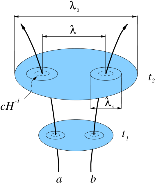
Figure 1: A schematic illustration of the separate universes picture, with the symbols as identified in the text.

Consider two such locally homogeneous regions $(a)$ and $(b)$ at fixed spatial coordinates, separated by a coordinate distance $\lambda$, on an initial hypersurface (e.g., uniform-density hypersurface) specified by a fixed coordinate time, $t=t_{1}$, in the appropriate gauge (e.g., uniform-density gauge). The initial large-scale curvature perturbation on the scale $\lambda$ can then be defined (independently of the background) as

$$\delta\psi_{1}\equiv\psi_{a1}-\psi_{b1}\,.$$ (2.217)

On a subsequent hypersurface defined by $t=t_{2}$ the curvature perturbation at $(a)$ or $(b)$ can be evaluated using Eq. (2.43) [but neglecting $\nabla^{2}\sigma$] to give [90]

$$\psi_{a2}=\psi_{a1}-\delta N_{a}\,,$$ (2.218)

where the integrated expansion between the two hypersurfaces along the world-line followed by region $(a)$ is given by $N_{a}=N+\delta N_{a}$, and $N\equiv\ln a$ is the expansion in the unperturbed background and

$$\delta N_{a}=\int_{1}^{2}{1\over 3}\delta\tilde{\theta}_{a}dt\,.$$ (2.219)

The curvature perturbation when $t=t_{2}$ on the comoving scale $\lambda$ is thus given by

$$\delta\psi_{2}\equiv\psi_{a2}-\psi_{b2}=\delta\psi_{1}-\left(N_{a}-N_{b}\right)\,.$$ (2.220)

In order to calculate the change in the curvature perturbation in any gauge on very large scales it is thus sufficient to evaluate the difference in the integrated expansion between the initial and final hypersurface along different world-lines.

In particular, using Eq. (2.220), one can evolve the curvature perturbation, $\zeta$, on super-horizon scales, knowing only the evolution of the family of Robertson–Walker universes, which according to the separate Universe assumption describe the evolution of the Universe on super-horizon scales:

$$-\Delta\zeta=-\Delta N\,.$$ (2.221)

where $-\zeta=\psi_{a}-\psi_{b}$ on uniform-density hypersurfaces and $\Delta N=N_{a}-N_{b}$ in Eq. (2.220). As we shall discuss in Section 4, this evolution is in turn specified by the values of the relevant fields during inflation, and as a result one can calculate $\zeta$ at horizon re-entry from the vacuum fluctuations of these fields.

While it is a non-trivial assumption to suppose that every comoving region well outside the horizon evolves like an unperturbed universe, there has to be some scale $\lambda_{\rm s}$ for which that assumption is true to useful accuracy. If there were not, the concept of an unperturbed (Robertson–Walker) background would make no sense. We use the phrase ‘background’ to describe the evolution on a much larger scale $\lambda_{0}$, which should be much bigger even than our present horizon size, with respect to which the perturbations in this section are defined. It is important to distinguish this from regions of size $\lambda_{\rm{s}}$ large enough to be treated as locally homogeneous, but which when pieced together over a larger scale, $\lambda$, represent the long-wavelength perturbations under consideration. Thus we require a hierarchy of scales:

$$\lambda_{0}\gg\lambda\gg\lambda_{{\rm s}}\gtrsim cH^{-1}\,.$$ (2.222)

Ideally $\lambda_{0}$ would be taken to be infinite. However it may be that the Universe becomes highly inhomogeneous on some very much larger scale, $\lambda_{{\rm e}}\gg\lambda_{0}$, where effects such as stochastic or eternal inflation determine the dynamical evolution. Nevertheless, this will not prevent us from defining an effectively homogeneous background in our observable Universe, which is governed by the local Einstein equations and hence impervious to anything happening on vast scales. Specifically we will assume that it is possible to foliate spacetime on this large scale $\lambda_{0}$ with spatial hypersurfaces.

When we use homogeneous equations to describe separate regions on length scales greater than $\lambda_{\rm{s}}$, we are implicitly assuming that the evolution on these scales is independent of shorter wavelength perturbations. This is true within linear perturbation theory in which the evolution of each Fourier mode can be considered independently, but any non-linear interaction introduces mode-mode coupling which undermines the separate universes picture. The separate universe model may still be used for the evolution of linear metric perturbation if the perturbations in the total density and pressure remain small, but a suitable model (possibly a thermodynamic description) of the effect of the non-linear evolution of matter fields on smaller scales may be necessary in some cases.

Adiabatic perturbations in the density and pressure correspond to shifts forwards or backwards in time along the background solution, $\delta p/\delta\rho={p^{\prime}}/\rho^{\prime}\equiv c_{s}^{2}$, and hence $\Gamma=0$ in Eq. (2.164). For example, in a universe containing only baryonic matter plus radiation, the density of baryons or photons may vary locally, but the perturbations are adiabatic if the ratio of photons to baryons remains unperturbed (cf. Eq.(2.215)). Different regions are compelled to undergo the same evolution along a unique trajectory in field space, separated only by a shift in the expansion. The pressure $p$ thus remains a unique function of the density $\rho$ and the energy conservation equation, $d\rho/dN=-3(\rho+p)$, determines $\rho$ as a function of the integrated expansion, $N$. Under these conditions, uniform-density hypersurfaces are separated by a uniform expansion and hence the curvature perturbation, $\zeta$, remains constant.

For $\Gamma\neq 0$ it is no longer possible to define a simple shift to describe both the density and pressure perturbation. The existence of a non-zero pressure perturbation on uniform-density hypersurfaces changes the equation of state in different regions of the Universe and hence leads to perturbations in the expansion along different worldlines between uniform-density hypersurfaces. This is consistent with Eq. (2.202) which quantifies how the non-adiabatic pressure perturbation determines the variation of $\zeta$ on large scales [30, 75].

We defined a generalized adiabatic condition which requires $\Gamma_{xy}=0$ for any physical scalars $x$ and $y$ in Eq. (2.165) in Section 2.10.6. In the separate universes picture this condition ensures that if all field perturbations are adiabatic at any one time (i.e. on any spatial hypersurface), then they must remain so on large scales at any subsequent time. Purely adiabatic perturbations can never give rise to entropy perturbations on large scales as all fields share the same time shift, $\delta\eta=\delta x/{x^{\prime}}$, along a single phase-space trajectory.

3 Quantum fluctuations from inflation

In this section we will discuss the generation of quantum fluctuations from inflation in the context of a particularly simple multi-component model: assisted inflation. The assisted inflation model is one of the very few models, in which it is possible to calculate the power spectra of the homogeneous and the inhomogeneous field fluctuations analytically, without resorting to the slow roll approximation [60, 75, 61].

3.1 The assisted inflation model

A single scalar field with an exponential potential is known to drive power-law inflation, where the cosmological scale factor grows as $a\propto t^{p}$ with $p>1$, for sufficiently flat potentials [69, 36, 14, 19]. Liddle, Mazumdar and Schunck [63] recently proposed a novel model of inflation driven by several scalar fields with exponential potentials. Although each separate potential,

$$V_{i}=V_{0}\exp\left(-\sqrt{16\pi\over p_{i}}{\varphi_{i}\over m_{\rm Pl}}\right)\,,$$ (3.1)

may be too steep to drive inflation by itself ($p_{i}<1$), the combined effect of several such fields, with total potential energy

$$V=\sum_{i=1}^{n}V_{i}\,,$$ (3.2)

leads to a power-law expansion $a\propto t^{\bar{p}}$ with [63]

$$\bar{p}=\sum_{i=1}^{n}p_{i}\,,$$ (3.3)

provided $\bar{p}>1/3$. Supergravity theories typically predict steep exponential potentials, but if many fields can cooperate to drive inflation, this may open up the possibility of obtaining inflationary solutions in such models.

Scalar fields with exponential potentials are known to possess self-similar solutions in Friedmann-Robertson-Walker models either in vacuum [36, 14] or in the presence of a barotropic fluid [106, 103, 19, 40]. In the presence of other matter, the scalar field is subject to additional friction, due to the larger expansion rate relative to the vacuum case. This means that a scalar field, even if it has a steep (non-inflationary) potential may still have an observable dynamical effect in a radiation or matter dominated era [107, 25, 26, 100].

The paper of Liddle, Mazumdar and Schunck [63] was the first to consider the effect of additional scalar fields with independent exponential potentials. They considered $n$ scalar fields in a spatially flat Friedmann-Robertson-Walker universe with scale factor $a(t)$. The Lagrange density for the fields, as an extension of Eq. (2.111), is

$${\cal L}=\sum_{i=1}^{n}-{1\over 2}\left(\nabla\varphi_{i}\right)^{2}-V_{i}\,,$$ (3.4)

with each exponential potential $V_{i}$ of the form given in Eq. (3.1). The cosmological expansion rate is then given by the Friedmann equation (2.83) in coordinate time

$$H^{2}={8\pi\over 3m_{\rm Pl}^{2}}\sum_{i=1}^{n}\left(V_{i}+{1\over 2}\dot{\varphi}_{i}^{2}\right)\,,$$ (3.5)

and the individual fields obey the Klein-Gordon equation (2.118),

$$\ddot{\varphi}_{i}+3H\dot{\varphi}_{i}=-{dV_{i}\over d\varphi_{i}}\,.$$ (3.6)

One can then obtain a scaling solution of the form [63]

$${\dot{\varphi}_{i}^{2}\over\dot{\varphi}_{j}^{2}}={V_{i}\over V_{j}}=C_{ij}\,.$$ (3.7)

Differentiating this expression with respect to time, and using the form of the potential given in Eq. (3.1) then implies that

$${1\over\sqrt{p_{i}}}\dot{\varphi}_{i}-{1\over\sqrt{p_{j}}}\dot{\varphi}_{j}=0\,,$$ (3.8)

and hence

$$C_{ij}={p_{i}\over p_{j}}\,.$$ (3.9)

The scaling solution is thus given by [63]

$${1\over\sqrt{p_{i}}}\varphi_{i}-{1\over\sqrt{p_{j}}}\varphi_{j}={m_{\rm Pl}\over\sqrt{16\pi}}\ln{p_{j}\over p_{i}}\,.$$ (3.10)

A numerical solution with four fields is shown in Fig. 2 as an example. In Ref. [63] the authors demonstrated the existence of a scaling solution for $n$ scalar fields written in terms of a single re-scaled field $\tilde{\varphi}=\sqrt{\bar{p}/p_{1}}\varphi_{1}$. The choice of $\varphi_{1}$ rather than any of the other fields is arbitrary as along the scaling solution all the $\varphi_{i}$ fields are proportional to one another.

Figure 2: Evolution of four fields $\varphi_{1}$, $\varphi_{2}$, $\varphi_{3}$ and $\varphi_{4}$ (from bottom to top) during assisted inflation with $p_{1}=0.3$, $p_{2}=1$, $p_{3}=2$ and $p_{4}=7$.

In this part of the thesis we will prove that this scaling solution is the late-time attractor by choosing a redefinition of fields (a rotation in field space) which allows us to write down the effective potential for field variations orthogonal to the scaling solution and show that this potential has a global minimum along the attractor solution. In general the full expression for an arbitrary number of fields is rather messy so we first give, in Section 3.2, the simplest case where there are just two fields, and then extend this to $n$ fields in Section 3.3. The resulting inflationary potential is similar to that used in models of hybrid inflation and we show in Section 3.4 that assisted inflation can be interpreted as a form of “hybrid power-law inflation”. As in the case of power-law or hybrid inflation, one can obtain analytic expressions for inhomogeneous linear perturbations close to the attractor trajectory without resorting to slow-roll type approximations. Thus we are able to give exact results for the large-scale perturbation spectra due to vacuum fluctuations in the fields in Section 3.5. We discuss our results in Sections 3.6 and 5.

3.2 Two field model

We will restrict our analysis initially to just two scalar fields, $\varphi_{1}$ and $\varphi_{2}$, with the Lagrange density

$${\cal L}=-{1\over 2}(\nabla\varphi_{1}^{2})-{1\over 2}(\nabla\varphi_{2}^{2})-V_{0}\left[\exp\left(-\sqrt{16\pi\over p_{1}}{\varphi_{1}\over m_{\rm Pl}}\right)+\exp\left(-\sqrt{16\pi\over p_{2}}{\varphi_{2}\over m_{\rm Pl}}\right)\right]\,.$$ (3.11)

We define the fields

$$\bar{\varphi}_{2} = {\sqrt{p_{1}}\varphi_{1}+\sqrt{p_{2}}\varphi_{2}\over\sqrt{p_{1}+p_{2}}}$$ (3.12)

$$+{m_{\rm Pl}\over\sqrt{16\pi(p_{1}+p_{2})}}\left(p_{1}\ln{p_{1}\over p_{1}+p_{2}}+p_{2}\ln{p_{2}\over p_{1}+p_{2}}\right)\,,$$

$$\bar{\sigma}_{2} = {\sqrt{p_{2}}\varphi_{1}-\sqrt{p_{1}}\varphi_{2}\over\sqrt{p_{1}+p_{2}}}+{m_{\rm Pl}\over\sqrt{16\pi}}\sqrt{p_{1}p_{2}\over p_{1}+p_{2}}\ln{p_{1}\over p_{2}}\,,$$ (3.13)

to describe the evolution along and orthogonal to the scaling solution, respectively, by applying a Gram-Schmidt orthogonalisation procedure.

Figure 3: The field rotation in the two field case. The $\bar{\varphi}_{2}$ direction is along the attractor, $\bar{\sigma}_{2}$ orthogonal to it.

The re-defined fields $\bar{\varphi}_{2}$ and $\bar{\sigma}_{2}$ are orthonormal linear combinations of the original fields $\varphi_{1}$ and $\varphi_{2}$. They represent a rotation, and arbitrary shift of the origin, in field-space. Fig. 3 illustrates this. Thus $\bar{\varphi}_{2}$ and $\bar{\sigma}_{2}$ have canonical kinetic terms, and the Lagrange density given in Eq. (3.11) can be written as

$${\cal L}=-{1\over 2}(\nabla\bar{\varphi}_{2}^{2})-{1\over 2}(\nabla\bar{\sigma}_{2}^{2})-\bar{V}(\bar{\sigma}_{2})\exp\left(-\sqrt{16\pi\over p_{1}+p_{2}}{\bar{\varphi}_{2}\over m_{\rm Pl}}\right)\,,$$ (3.14)

where

$$\bar{V}(\bar{\sigma}_{2}) = V_{0}\left[{p_{1}\over p_{1}+p_{2}}\exp\left(-\sqrt{16\pi\over p_{1}+p_{2}}\sqrt{p_{2}\over p_{1}}{\bar{\sigma}_{2}\over m_{\rm Pl}}\right)\right.$$ (3.15)

$$+\left.{p_{2}\over p_{1}+p_{2}}\exp\left(\sqrt{16\pi\over p_{1}+p_{2}}\sqrt{p_{1}\over p_{2}}{\bar{\sigma}_{2}\over m_{\rm Pl}}\right)\right]\,.$$

It is easy to confirm that $\bar{V}(\bar{\sigma}_{2})$ has a global minimum value $V_{0}$ at $\bar{\sigma}_{2}=0$, which implies that $\bar{\sigma}_{2}=0$ is the late time attractor, which coincides with the scaling solution given in Eq. (3.10) for two fields.

Close to the scaling solution we can expand about the minimum, to second-order in $\bar{\sigma}_{2}$, and we obtain

$$V(\bar{\varphi}_{2},\bar{\sigma}_{2})\approx V_{0}\left[1+{8\pi\over(p_{1}+p_{2})}{\bar{\sigma}_{2}^{~{}2}\over m_{\rm Pl}^{2}}\right]\exp\left(-\sqrt{16\pi\over p_{1}+p_{2}}{\bar{\varphi}_{2}\over m_{\rm Pl}}\right)\,.$$ (3.16)

Note that the potential for the field $\bar{\sigma}_{2}$ has the same form as in models of hybrid inflation [66, 67, 20] where the inflaton field rolls towards the minimum of a potential with non-vanishing potential energy density ${V}_{0}$. Here there is in addition a “dilaton” field, $\bar{\varphi}_{2}$, which leads to a time-dependent potential energy density as $\bar{\sigma}_{2}\to 0$. Assisted inflation is related to hybrid inflation [66, 67, 20] in the same way that extended inflation [58] was related to Guth’s old inflation model [34]. As in hybrid or extended inflation, we require a phase transition to bring inflation to an end. Otherwise the potential given by Eq. (3.16) leads to inflation into the indefinite future.

3.3 Many field model

We will now prove that the attractor solution presented in Ref. [63] is the global attractor for an arbitrary number of fields with exponential potentials of the form given in Eq. (3.1), using proof by induction. To do this, we recursively construct the orthonormal fields and their potential.

Let us assume that we already have $n$ fields $\varphi_{i}$ with exponential potentials $V_{i}$ of the form given in Eq. (3.1) and that it is possible to pick $n$ orthonormal fields $\bar{\sigma}_{2},\ldots,\bar{\sigma}_{n}$ and $\bar{\varphi}_{n}$ such that the sum of the individual potentials $V_{i}$ can be written as

$$\sum_{i=1}^{n}V_{i}=\bar{V}_{n}\exp\left(-\sqrt{16\pi\over\bar{p}_{n}}{\bar{\varphi}_{n}\over m_{\rm Pl}}\right)\,,$$ (3.17)

where we will further assume that $\bar{V}_{n}=\bar{V}_{n}(\bar{\sigma}_{i})$ has a global minimum $\bar{V}_{n}(0)=V_{0}$ when $\bar{\sigma}_{i}=0$ for all $i$ from $2$ to $n$.

It is possible to extend this form of the potential to $n+1$ fields if we consider an additional field $\varphi_{n+1}$ with an exponential potential $V_{n+1}$ of the form given in Eq. (3.1). Analogously to the two field case, we define

$$\bar{\varphi}_{n+1} = {\sqrt{\bar{p}_{n}}\bar{\varphi}_{n}+\sqrt{p_{n+1}}\varphi_{n+1}\over\sqrt{\bar{p}_{n+1}}}$$ (3.18)

$$+ {m_{\rm Pl}\over\sqrt{16\pi(\bar{p}_{n+1})}}\left(\bar{p}_{n}\ln{\bar{p}_{n}\over\bar{p}_{n+1}}+p_{n+1}\ln{p_{n+1}\over\bar{p}_{n+1}}\right)\,,$$

$$\bar{\sigma}_{n+1} = {\sqrt{p_{n+1}}\bar{\varphi}_{n}-\sqrt{\bar{p}_{n}}\varphi_{n+1}\over\sqrt{\bar{p}_{n+1}}}+{m_{\rm Pl}\over\sqrt{16\pi}}\sqrt{\bar{p}_{n}p_{n+1}\over\bar{p}_{n+1}}\ln{\bar{p}_{n}\over p_{n+1}}\,,$$ (3.19)

where

$$\bar{p}_{n+1}=\bar{p}_{n}+p_{n+1}\ .$$ (3.20)

Using these definitions we can show that the sum of the $n+1$ individual potentials $V_{i}$ can be written as

$$\sum_{i=1}^{n+1}V_{i}=\bar{V}_{n+1}\exp\left(-\sqrt{16\pi\over\bar{p}_{n+1}}{\bar{\varphi}_{n+1}\over m_{\rm Pl}}\right)\,,$$ (3.21)

where $\bar{V}_{n+1}=\bar{V}_{n+1}(\bar{\sigma}_{i})$ is given by

$$\bar{V}_{n+1} = \bar{V}_{n}{\bar{p}_{n}\over\bar{p}_{n+1}}\exp\left(-\sqrt{16\pi\over\bar{p}_{n+1}}\sqrt{p_{n+1}\over\bar{p}_{n}}{\bar{\sigma}_{n+1}\over m_{\rm Pl}}\right)$$ (3.22)

$$+ V_{0}~{}{p_{n+1}\over\bar{p}_{n+1}}\exp\left(\sqrt{16\pi\over\bar{p}_{n+1}}\sqrt{\bar{p}_{n}\over p_{n+1}}{\bar{\sigma}_{n+1}\over m_{\rm Pl}}\right)\,.$$

Because we have assumed that $\bar{V}_{n}$ has a global minimum value $\bar{V}_{n}(0)=V_{0}$ when $\bar{\sigma}_{i}=0$ for all $i$ from $2$ to $n$, one can verify that $\bar{V}_{n+1}$ also has a minimum value $\bar{V}_{n+1}(0)=V_{0}$ when $\bar{\sigma}_{i}=0$, for all $i$ from $2$ to $n+1$.

However, we have already shown in Section 3.2 that for two fields $\varphi_{1}$ and $\varphi_{2}$, we can define two fields $\bar{\varphi}_{2}$ and $\bar{\sigma}_{2}$, given in Eqs. (3.12) and (3.13) whose combined potential given in Eq. (3.14) is of the form required in Eq. (3.17), with $\bar{p}_{2}=p_{1}+p_{2}$. Hence we can write the potential in the form given in Eq. (3.17) for $n$ fields, for all $n\geq 2$, with

$$\bar{p}\equiv\bar{p}_{n}=\sum_{i=1}^{n}p_{i}\ .$$ (3.23)

Equations (3.12) and (3.18) then lead us to the non-recursive expression for the “weighted mean field”

$$\bar{\varphi}\equiv\bar{\varphi}_{n}=\sum_{i=1}^{n}\left(\sqrt{{p_{i}\over\bar{p}}}\varphi_{i}+{m_{\rm Pl}\over\sqrt{16\pi\bar{p}}}~{}p_{i}\ln{p_{i}\over\bar{p}}\right)\,,$$ (3.24)

which describes the evolution along the scaling solution. This is simply a rotation in field space plus an arbitrary shift, chosen to preserve the form of the potential given in Eq. (3.17). The $n-1$ fields $\bar{\sigma}_{i}$ describe the evolution orthogonal to the attractor trajectory.

The potential $\bar{V}_{n}$ has a global minimum at $\bar{\sigma}_{i}=0$, which demonstrates that this is the stable late-time attractor. From Eqs. (3.15) and (3.22) we get a closed expression for $\bar{V}_{n}$,

$$\bar{V}_{n} = V_{0}\left\{\frac{p_{1}}{\bar{p}}\exp\left[-\frac{\sqrt{16\pi}}{m_{\rm Pl}}~{}\sum^{n}_{i=2}\sqrt{\frac{p_{i}}{\bar{p}_{i}\bar{p}_{i-1}}}~{}\bar{\sigma}_{i}\right]\right.$$ (3.25)

$$+ \left.~{}\sum^{n-1}_{i=2}\frac{p_{i}}{\bar{p}}\exp\left[\frac{\sqrt{16\pi}}{m_{\rm Pl}}\left(\sqrt{\frac{\bar{p}_{i-1}}{\bar{p}_{i}p_{i}}}~{}\bar{\sigma}_{i}-\sum^{n}_{j=i+1}\sqrt{\frac{p_{j}}{\bar{p}_{j}\bar{p}_{j-1}}}~{}\bar{\sigma}_{j}\right)\right]\right.$$

$$\qquad\left.+~{}\frac{p_{n}}{\bar{p}}\exp\left[\frac{\sqrt{16\pi}}{m_{\rm Pl}}\sqrt{\frac{\bar{p}_{n-1}}{\bar{p}p_{n}}}~{}\bar{\sigma}_{n}\right]\right\}.$$

Close to the attractor trajectory (to second order in $\bar{\sigma}_{i}$) we can write a Taylor expansion for the potential

$$\sum_{i=1}^{n}V_{i}\approx V_{0}\left(1+{8\pi\over{\bar{p}m_{\rm Pl}^{2}}}\sum_{j=2}^{n}\bar{\sigma}_{j}^{2}\right)\exp\left(-\sqrt{16\pi\over\bar{p}}{\bar{\varphi}_{n}\over m_{\rm Pl}}\right)\,.$$ (3.26)

Note that this expression is dependent only upon $\bar{p}$ and not on the individual $p_{i}$.

3.4 Stringy hybrid inflation

The form of the potentials in Eqs. (3.16) and (3.26) is reminiscent of the effective potential obtained in the Einstein conformal frame from Brans-Dicke type gravity theories [102]. The appearance of the weighted mean field, $\bar{\varphi}$, as a “dilaton” field in the potential suggests that the matter Lagrangian might have a simpler form in a conformally related frame. If we work in terms of a conformally re-scaled metric

$$\tilde{g}_{\mu\nu}=\exp\left(-\sqrt{16\pi\over\bar{p}}{\bar{\varphi}\over m_{\rm Pl}}\right)g_{\mu\nu}\,,$$ (3.27)

then the Lagrange density given in Eq. (3.14) becomes

$$\tilde{{\cal L}}=\exp\left(\sqrt{16\pi\over\bar{p}}{\bar{\varphi}\over m_{\rm Pl}}\right)\times\left\{-{1\over 2}\left(\tilde{\nabla}\bar{\varphi}\right)^{2}-\sum_{i=2}^{n}{1\over 2}\left(\tilde{\nabla}\bar{\sigma}_{i}\right)-\bar{V}\right\}\,,$$ (3.28)

In this conformal related frame the field $\bar{\varphi}$ is non-minimally coupled to the gravitational part of the Lagrangian. The original field equations were derived from the full action, including the Einstein-Hilbert Lagrangian of general relativity,

$$S=\int d^{4}x\sqrt{-g}\left[{m_{\rm Pl}^{2}\over 16\pi}R+{\cal L}\right]\,,$$ (3.29)

where $R$ is the Ricci scalar curvature of the metric $g_{\mu\nu}$. In terms of the conformally related metric given in Eq. (3.27) this action becomes (up to boundary terms [104])

$$S=\int d^{4}x\sqrt{-\tilde{g}}e^{-\varphi_{\rm{dil}}}\left[{m_{\rm Pl}^{2}\over 16\pi}\tilde{R}-\omega(\tilde{\nabla}\varphi_{\rm{dil}})-{1\over 2}\sum_{i=1}^{n-1}(\tilde{\nabla}\bar{\sigma}_{i})^{2}-\bar{V}\right]\,,$$ (3.30)

where we have introduced the dimensionless dilaton field

$$\varphi_{\rm{dil}}=-\sqrt{16\pi\over\bar{p}}{\bar{\varphi}\over m_{\rm Pl}}\,,$$ (3.31)

and the dimensionless Brans-Dicke parameter

$$\omega={\bar{p}-3\over 2}\,.$$ (3.32)

Thus the assisted inflation model is identical to $n-1$ scalar fields $\bar{\sigma}_{i}$ with a hybrid inflation type potential $\bar{V}(\bar{\sigma}_{i})$ in a string-type gravity theory with dilaton, $\varphi_{\rm{dil}}\propto\bar{\varphi}$. However, we note that in order to obtain power-law inflation with $\bar{p}\gg 1$ the dimensionless constant $\omega$ must be much larger than that found in the low-energy limit of string theory where $\omega=-1$.

3.5 Perturbations about the attractor

The redefined orthonormal fields and the potential allow us to give the equations of motion for the independent degrees of freedom. If we consider only linear perturbations about the attractor then the energy density is independent of all the fields except $\bar{\varphi}$, and we can solve the equation for the $\bar{\varphi}$ field analytically.

The field equation for the weighted mean field is

$$\ddot{\bar{\varphi}}+3H\dot{\bar{\varphi}}=\sqrt{{16\pi\over\bar{p}}}{V\over m_{\rm Pl}}\,.$$ (3.33)

Along the line $\bar{\sigma}_{i}=0$ for all $i$ in field space, we have

$$V=V_{0}\exp\left(-\sqrt{16\pi\over\bar{p}}{\bar{\varphi}\over m_{\rm Pl}}\right)\,,$$ (3.34)

and the well-known power-law solution [69] with $a\propto t^{\bar{p}}$ is the late-time attractor [36, 14] for this potential, where

$$\bar{\varphi}(t)=\bar{\varphi}_{0}\ln\left(\frac{t}{t_{0}}\right),$$ (3.35)

and $\bar{\varphi}_{0}=m_{\rm{Pl}}\sqrt{\bar{p}/4\pi}$ and $t_{0}=m_{\rm{Pl}}\sqrt{\bar{p}/8\pi V_{0}(3\bar{p}-1)}$.

3.5.1 Homogeneous linear perturbations

The field equations for the $\bar{\sigma}_{i}$ fields are

$$\ddot{\bar{\sigma}_{i}}+3H\dot{\bar{\sigma}_{i}}+\frac{\partial V}{\partial\bar{\sigma}_{i}}=0.$$ (3.36)

where the potential $V$ is given by Eqs. (3.17) and (3.25), and the attractor solution corresponds to $\bar{\sigma}_{i}=0$. Equation (3.26) shows that we can neglect the back-reaction of $\bar{\sigma}_{i}$ upon the energy density, and hence the cosmological expansion, to first-order and the field equations have the solutions

$$\bar{\sigma}_{i}(t)=\Sigma_{i+}t^{s_{+}}+\Sigma_{i-}t^{s_{-}},$$ (3.37)

where

$$s_{\pm}=\frac{3\bar{p}-1}{2}\left[-1\pm\sqrt{\frac{3(\bar{p}-3)}{3\bar{p}-1}}~{}\right],$$ (3.38)

for $\bar{p}>3$, confirming that $\sigma_{i}=0$ is indeed a local attractor. In the limit $\bar{p}\to\infty$ we obtain $s_{i}=-2$. For $1<\bar{p}<3$ the perturbations are under-damped and execute decaying oscillations about $\bar{\sigma}_{i}=0$.

The form of the solutions given in Eq. (3.37) for $\bar{\sigma}_{i}(t)$ close to the attractor is the same for all the orthonormal fields $\bar{\sigma}_{i}$, as demonstrated in Fig. 4. Their evolution is independent of the individual $p_{i}$ and determined only by the sum, $\bar{p}$, as expected from the form of the potential given in Eq. (3.26).

Figure 4: Evolution of the fields $\bar{\sigma}_{1}$, $\bar{\sigma}_{2}$, and $\bar{\sigma}_{3}$, orthogonal to the scaling solution, in the assisted inflation model shown in Fig. 2.

3.5.2 Inhomogeneous Linear Perturbations

Conventional hybrid inflation and power-law inflation are two of the very few models [60] in which one can obtain exact analytic expressions for the spectra of vacuum fluctuations on all scales without resorting to a slow-roll type approximation. In the case of hybrid inflation, this is only possible in the limit that the inflaton field $\sigma$ approaches the minimum of its potential and we can neglect its back-reaction on the metric [30]. As the present model is so closely related to both power-law and hybrid inflation models close to the attractor, it is maybe not surprising then that we can obtain exact expressions for the evolution of inhomogeneous linear perturbations close to the scaling solution.

We will work in terms of the redefined fields $\bar{\varphi}$ and $\bar{\sigma}_{i}$, and their perturbations on spatially flat hypersurfaces [79]. In the limit that $\bar{\sigma}_{i}\to 0$ we can neglect the back-reaction of the $\bar{\sigma}_{i}$ field upon the metric and the field $\bar{\varphi}$. Perturbations in the field $\bar{\varphi}$ then obey the usual equation for a single field driving inflation [83], and perturbations in the field $\bar{\sigma}_{i}$ evolve in a fixed background. Defining

$$u = a\delta\bar{\varphi}\,,$$ (3.39)

$$\bar{v}_{i} = a\delta\bar{\sigma}_{i}\,,$$ (3.40)

we obtain the decoupled equations of motion for perturbations with comoving wavenumber $k$,

$$u_{k}^{\prime\prime}+\left(k^{2}-{z^{\prime\prime}\over z}\right)u_{k} = 0\,,$$ (3.41)

$$\bar{v}_{ik}^{\prime\prime}+\left(k^{2}+a^{2}{d^{2}V\over d\bar{\sigma}_{i}^{2}}-{a^{\prime\prime}\over a}\right)\bar{v}_{ik} = 0\,,$$ (3.42)

where [83] $z\equiv a^{2}\bar{\varphi}^{\prime}/a^{\prime}$ and a prime denotes differentiation with respect to conformal time $\eta\equiv\int dt/a$. For power-law expansion we have $z\propto a\propto(-\eta)^{-\bar{p}/(\bar{p}-1)}$ and thus

$${a^{\prime\prime}\over a}={\bar{p}(2\bar{p}-1)\over(\bar{p}-1)^{2}}~{}\eta^{-2}.$$ (3.43)

We also have $aH\propto-\bar{p}/((\bar{p}-1)\eta)$ which gives

$$a^{2}{d^{2}V\over d\sigma^{2}}=\frac{2(3\bar{p}-1)}{(\bar{p}-1)^{2}}~{}\eta^{-2},$$ (3.44)

where we have used the fact that $d^{2}V/d\bar{\sigma}_{i}^{2}=16\pi V/m_{\rm Pl}^{2}$ along the attractor. The equations of motion therefore become

$$u_{k}^{\prime\prime}+\left(k^{2}-{\nu^{2}-(1/4)\over\eta^{2}}\right)u_{k} = 0\,,$$ (3.45)

$$\bar{v}_{ik}^{\prime\prime}+\left(k^{2}-{\lambda^{2}-(1/4)\over\eta^{2}}\right)\bar{v}_{ik} = 0\,,$$ (3.46)

where

$$\nu = {3\over 2}+{1\over\bar{p}-1}\,,$$ (3.47)

$$\lambda = {3\over 2}{\sqrt{(\bar{p}-3)(\bar{p}-1/3)}\over\bar{p}-1}\,,$$ (3.48)

and the general solutions in terms of Hankel functions are

$$u_{k}=U_{1}(-k\eta)^{1/2}H^{(1)}_{\nu}(-k\eta)+U_{2}(-k\eta)^{1/2}H^{(2)}_{\nu}(-k\eta)\,,$$ (3.49)

$$\bar{v}_{ik}=V_{1i}(-k\eta)^{1/2}H^{(1)}_{\lambda}(-k\eta)+V_{2i}(-k\eta)^{1/2}H^{(2)}_{\lambda}(-k\eta)\,.$$ (3.50)

Taking only positive frequency modes in the initial vacuum state for $|k\eta|\gg 1$ and normalising requires $u_{k}$ and $\bar{v}_{ik}\to e^{-ik\eta}/\sqrt{2k}$, which gives the vacuum solutions

$$u_{k} = \frac{1}{2}(-\pi\eta)^{1/2}e^{\frac{\pi}{2}(\nu+1)i}H^{(1)}_{\nu}(-k\eta),$$ (3.51)

$$\bar{v}_{ik} = \frac{1}{2}(-\pi\eta)^{1/2}e^{\frac{\pi}{2}(\lambda+1)i}H^{(1)}_{\lambda}(-k\eta),$$ (3.52)

In the opposite limit, i.e., $-k\eta\to 0$, we use the limiting form of the Hankel functions, $H_{\nu}^{(1)}(z)\sim-(i/\pi)\Gamma(\nu)z^{-\nu}$, and therefore on large scales, and at late times, we obtain

$$u_{k} \to \frac{2^{\nu-1}}{\sqrt{\pi k}}e^{i\frac{\pi}{2}\nu}\left(-k\eta\right)^{\frac{1}{2}-\nu}\Gamma(\nu),$$ (3.53)

$$\bar{v}_{ik} \to \frac{2^{\lambda-1}}{\sqrt{\pi k}}e^{i\frac{\pi}{2}\lambda}\left(-k\eta\right)^{\frac{1}{2}-\lambda}\Gamma(\lambda)\,.$$ (3.54)

The power spectrum of a Gaussian random field $X$ is conventionally given by [61]

$${\cal P}_{X}(k)\equiv\left(\frac{k^{3}}{2\pi^{2}}\right)|X_{k}|^{2}\,.$$ (3.55)

The power spectra on large scales for the field perturbations $\delta\bar{\varphi}$ and $\delta\bar{\sigma}_{i}$ are thus

$${\cal P}_{\delta\varphi}^{~{}~{}1/2} = \frac{C(\nu)}{\left(\nu-\frac{1}{2}\right)}~{}\frac{H}{2\pi}~{}\left(-k\eta\right)^{\frac{3}{2}-\nu},$$ (3.56)

$${\cal P}_{\delta\sigma_{i}}^{~{}~{}1/2} = \frac{C(\lambda)}{\left(\nu-\frac{1}{2}\right)}~{}\frac{H}{2\pi}~{}\left(-k\eta\right)^{\frac{3}{2}-\lambda},$$ (3.57)

where we have used $\eta=-(\nu-1/2)/(aH)$ and we define

$$C(\alpha)\equiv\frac{2^{\alpha}\Gamma(\alpha)}{2^{\frac{3}{2}}\Gamma(\frac{3}{2})}.$$ (3.58)

Both the weighted mean field $\bar{\varphi}$ and the orthonormal fields $\bar{\sigma}_{i}$ are “light” fields ($m^{2}<3H^{2}/2$) during assisted inflation (for $\bar{p}>3$) and thus we obtain a spectrum of fluctuations in all the fields on large scales. Note that in the de Sitter limit, $\bar{p}\to\infty$ and thus $\nu\to 3/2$ and $\lambda\to 3/2$, we have ${\cal P}_{\delta\varphi}^{~{}1/2}\to H/2\pi$, and ${\cal P}_{\delta\sigma_{i}}^{~{}1/2}\to H/2\pi$.

Denoting the scale dependence of the perturbation spectra by

$$\Delta n_{x}\equiv\frac{d\ln{\cal P}_{x}}{d\ln k}\,,$$ (3.59)

we obtain

$$\Delta n_{\delta\varphi} = 3-2\nu=-\frac{2}{\bar{p}-1},$$ (3.60)

$$\Delta n_{\delta\bar{\sigma}_{i}} = 3-2\lambda=3\left(1-{\sqrt{(\bar{p}-3)(\bar{p}-1/3)}\over\bar{p}-1}\right).$$ (3.61)

3.6 Conclusions

We have shown that the assisted inflation model, driven by many scalar fields with steep exponential potentials, can be better understood by performing a rotation in field space, which allows us to re-write the potential as a product of a single exponential potential for a weighted mean field, $\bar{\varphi}$, and a potential $\bar{V}_{n}$ for the orthogonal degrees of freedom, $\bar{\sigma}_{i}$, which has a global minimum when $\bar{\sigma}_{i}=0$. This proves that the scaling solution found in Ref. [63] is indeed the late-time attractor.

The particular form of the potential which we present for scalar fields minimally-coupled to the spacetime metric, can also be obtained via a conformal transformation of a hybrid inflation type inflationary potential [66, 67, 20] with a non-minimally coupled, but otherwise massless, dilaton field, $\varphi_{\rm{dil}}\propto\bar{\varphi}$. Thus we see that assisted inflation can be understood as a form of power-law hybrid inflation, where the false-vacuum energy density is diluted by the evolution of the dilaton field.

We have also been able to give exact solutions for inhomogeneous linear perturbations about the attractor trajectory in terms of our rotated fields. Perturbations in the weighted mean field $\bar{\varphi}$ corresponds to the perturbations in the density on the uniform curvature hypersurfaces, or equivalently, perturbations in the curvature of uniform density hypersurfaces:

$$\zeta=-{H\over\dot{\bar{\varphi}}}\delta\bar{\varphi}\,.$$ (3.62)

These perturbations are along the attractor trajectory, and hence describe adiabatic curvature perturbations. The perturbation spectrum for $\zeta$ is

$${\cal P}_{\zeta}=\left(\frac{H}{\dot{\bar{\varphi}}}\right)^{2}{\cal P}_{\delta\varphi}$$ (3.63)

which will be ${\cal P}_{\zeta}^{1/2}=H^{2}/(2\pi\dot{\bar{\varphi}})$ in the de Sitter limit (where $\bar{p}\to\infty$). The spectral index of the curvature perturbations on large scales is thus given from Eq. (3.60) as

$$n_{s}\equiv 1+{d\ln{\cal P}_{\zeta}\over d\ln k}=1-{2\over\bar{p}-1}\,,$$ (3.64)

and is always negatively tilted with respect to the Harrison-Zel’dovich spectrum where $n_{s}=1$. Note that in the de Sitter limit ($\bar{p}\to\infty$) we recover the result of Ref. [63].

First-order perturbations in the fields orthogonal to the weighted mean field are isocurvature perturbations during inflation. Vacuum fluctuations lead to a positively tilted spectrum. The presence of non-adiabatic perturbations can lead to a more complicated evolution of the large-scale curvature perturbation than may be assumed in single-field inflation models [92, 90, 29] as discussed in Section 2 and in particular Section 2.12. However, we have shown that these perturbations decay relative to the adiabatic perturbations and hence we recover the single field limit at late times. In particular we find that the curvature perturbation $\zeta$ becomes constant on super-horizon scales during inflation. Note, however, that assisted inflation must be ended by a phase transition whose properties are not specified in the model. If this phase transition is sensitive to the isocurvature (non-adiabatic) fluctuations orthogonal to the attractor trajectory, then the curvature perturbation, $\zeta$, during the subsequent radiation dominated era may not be simply related to the curvature perturbation during inflation.

Since the publication of the first two papers on assisted inflation, [63, 79], the model has enjoyed considerable further interest by several authors. In Ref. [21], Copeland, Mazumdar and Nunes extended the model presented above to include cross-couplings between the scalar fields. Kanti and Olive proposed a realisation of assisted inflation based on the compactification of a five-dimensional Kaluza-Klein model, extending the model to include standard chaotic-type potentials [52, 53]. Green and Lidsey showed that an arbitrary number of scalar fields with exponential potentials can be obtained from compactification of a higher dimensional theory [32]. They used a rotation in field space to show that the system reduces to a single scalar field with a single exponential potential. Coley and van den Hoogen investigated the dynamics of assisted inflation, including a barotropic fluid and curvature as well as scalar fields with exponential potentials, applying methods of dynamical systems [18]. Lately Kaloper and Liddle used the assisted inflation mechanism in connection with chaotic inflation and showed that the dynamics does not become independent of the initial conditions at late times [51].

4 Preheating

The standard inflationary paradigm is an extremely successful model in explaining observed structures in the Universe (see Refs. [60, 61, 75] for reviews). The inhomogeneities originate from the quantum fluctuations of the inflaton field, which on being stretched to large scales become classical perturbations as shown in the preceding section. The field inhomogeneities generate a perturbation in the curvature of uniform density hypersurfaces, $\zeta$, as shown in the preceding section and later on these inhomogeneities are inherited by matter and radiation when the inflaton field decays. In the simplest scenario, the curvature perturbation on scales much larger than the Hubble length is constant, and in particular is unchanged during the inflaton decay. This enables a prediction of the present-day perturbations which does not depend on the specific cosmological evolution between the late stages of inflation and the recent past (say, before nucleosynthesis).

It has recently been claimed [5, 6] that this simple picture may be violated if inflation ends with a period of preheating, a violent decay of the inflaton particles into another field (or even into quanta of the inflaton field itself). Such a phenomenon would completely undermine the usual inflationary picture, and indeed the original claim was that large-scale perturbations would be amplified into the non-linear regime, placing them in conflict with observations such as measurements of microwave background anisotropies. Given the observational successes of the standard picture, these claims demand attention.

In Section 2.12.2 and Ref. [105], we discuss the general criteria under which large-scale curvature perturbations can vary. As has been known for some time, this is possible provided there exist large-scale non-adiabatic pressure perturbations, as can happen for example in multi-field inflation models [95, 28, 30, 90, 75]. Under those circumstances a significant effect is possible during preheating, though there is nothing special about the preheating era in this respect and this effect always needs to be considered in any multi-component inflation model.

In this section we perform an analysis of the simplest preheating model, as discussed in Ref. [5, 6]. We identify two possible sources of variation of the curvature perturbation. One comes from large-scale isocurvature perturbations in the preheating field into which the inflaton decays; we concur with the recent analyses of Jedamzik and Sigl [50] and Ivanov [49] that this effect is negligible due to the rapid decay of the background value of the preheating field during inflation. However, we also show that in fact a different mechanism gives the dominant contribution, which is second-order in the field perturbations coming from short-wavelength fluctuations in the fields. Nevertheless, we show too that this effect is completely negligible, and hence that preheating in this model has no significant effect on large-scale curvature perturbations.

4.1 Perturbation evolution

We describe the perturbations via the curvature perturbation on uniform-density hypersurfaces, denoted $\zeta$ . In linear theory the evolution of $\zeta$ is well known, and arises from the non-adiabatic part of the pressure perturbations, Eq. (2.164).

On large scales anisotropic stress can be ignored when the matter content is entirely in the form of scalar fields, and in its absence the non-adiabatic pressure perturbation determines the variation of $\zeta$, and rewriting Eq. (2.202) we get [30, 75]

$${d\zeta\over dN}=-\frac{1}{\rho+p}\,\delta p_{\rm{nad}}\,,$$ (4.1)

where $N\equiv\ln a$ measures the integrated expansion. The uniform-density hypersurfaces become ill-defined [cf. the definition of $\zeta$, Eq. (2.78)] if the density is not a strictly decreasing function along worldlines between hypersurfaces of uniform density, and one might worry that this undermines the above analysis. However we can equally well derive this evolution equation in terms of the density perturbation on spatially-flat hypersurfaces, $\delta\rho_{\psi}\equiv-(d\rho/dN)\zeta$, which remains well-defined. Spatially-flat hypersurfaces are automatically separated by a uniform integrated expansion on large scales, so the perturbed continuity equation in this gauge takes the particularly simple form

$${d\delta\rho_{\psi}\over dN}=-3(\delta\rho_{\psi}+\delta p_{{\psi}})\,.$$ (4.2)

From this one finds that $\delta\rho_{\psi}\propto d\rho/dN$ for adiabatic perturbations and hence again we recover a constant value for $\zeta$. However it is clearly possible for entropy perturbations to cause a change in $\zeta$ on arbitrarily large scales when the non-adiabatic pressure perturbation is non-negligible.

4.2 Preheating

During inflation, the reheat field into which the inflaton field decays possesses quantum fluctuations on large scales just like the inflaton field itself. As these perturbations are uncorrelated with those in the inflaton field, the adiabatic condition will not be satisfied, and hence there is a possibility that $\zeta$ might vary on large scales. Only direct calculation can demonstrate whether the effect might be significant, and we now compute this effect in the simplest preheating model, as analyzed in Ref. [5, 6]. This is a chaotic inflation model with scalar field potential

$$V(\varphi,\chi)=\frac{1}{2}\,m^{2}\varphi^{2}+\frac{1}{2}\,g^{2}\varphi^{2}\chi^{2}\,,$$ (4.3)

where $\varphi$ is the inflaton and $\chi$ the reheat field, and $m$ and $g$ are the inflaton mass and the coupling of the reheat field to the inflaton, respectively. Slow-roll inflation proceeds with $\varphi\gtrsim m_{{\rm Pl}}$ and $g\chi\ll m$. The effective mass of the $\chi$ field is $g\varphi$ and thus will be much larger than the Hubble rate, $H\simeq\sqrt{4\pi/3}\,m\varphi/m_{{\rm Pl}}$, for $g\gg m/m_{{\rm Pl}}\sim 10^{-6}$. Throughout this section, we use the symbol ‘$\simeq$’ to indicate equality within the slow-roll approximation.

This model gives efficient preheating, since the effective mass of $\chi$ oscillates about zero with large amplitude. In most other models of inflation, preheating is less efficient or absent, because the mass oscillates about a nonzero value and/or has a small amplitude.

Any variation of $\zeta$ during preheating will be driven by the (non-adiabatic part of) the $\chi$ field perturbation. Our calculation takes place in three steps. The first is to compute the perturbations in the $\chi$ field at the end of inflation. The second is to compute how these perturbations are amplified during the preheating epoch by the strong resonance. Finally, the main part of the calculation is to compute the change in $\zeta$ driven by these $\chi$ perturbations.

4.2.1 The initial quantum fluctuation of the $\chi$-field

Perturbations in the $\chi$ field obey the wave equation

$$\ddot{\delta\chi}+3H\dot{\delta\chi}+\left(\frac{k^{2}}{a^{2}}+g^{2}\varphi^{2}\right)\delta\chi=0\,.$$ (4.4)

The slow-roll conditions ensure that the $\chi$ field remains in the adiabatic vacuum state for a massive field [10]

$$\delta\chi_{k}\simeq{a^{-\frac{3}{2}}~{}e^{-i\omega t}\over\sqrt{2\omega}}\,,$$ (4.5)

where $\omega^{2}=k^{2}/a^{2}+g^{2}\varphi^{2}$. This is an approximate solution to Eq. (4.4) provided

$$\nu\equiv\frac{m_{\chi}}{H}\simeq\sqrt{\frac{3}{4\pi}}\frac{g\,m_{{\rm Pl}}}{m}\gg 1\,,$$ (4.6)

where $m_{\chi}\equiv g\varphi$ is the effective mass of the $\chi$ field.

Hence the power spectrum (defined in Eq. (3.55)) for long-wavelength fluctuations ($k\ll m_{\chi}$) in the $\chi$ field simply reduces to the result for massive field in flat space

$${\cal P}_{\delta\chi}\simeq\frac{1}{4\pi^{2}m_{\chi}}\left(\frac{k}{a}\right)^{3}\,.$$ (4.7)

Physically, this says that at all times the expansion of the Universe has a negligible effect on the modes as compared to the mass. In particular, at the end of inflation we can write

$$\left.{\cal P}_{\delta\chi}\right|_{{\rm end}}\simeq\frac{1}{\nu}\left(\frac{H_{{\rm end}}}{2\pi}\right)^{2}\left(\frac{k}{k_{{\rm end}}}\right)^{3}\,.$$ (4.8)

The power spectrum has a spectral index $n_{{}_{\delta\chi}}=3$. This is the extreme limit of the mechanism used to give a blue tilt in isocurvature inflation scenarios [68, 87].

4.2.2 Parametric resonance

After inflation, the inflaton field $\varphi$ oscillates. Strong parametric resonance may now occur, amplifying the initial quantum fluctuation in $\chi$ to become a perturbation of the classical field $\chi$. The condition for this is

$$q\equiv\frac{g^{2}\varphi_{\rm{ini}}^{2}}{4m^{2}}\gg 1\,,$$ (4.9)

where $\varphi_{\rm{ini}}$ is the initial amplitude of the $\varphi$-field oscillations.

We model the effect of preheating on the amplitude of the $\chi$ field following Ref. [57] as

$${\cal P}_{\delta\chi}=\left.{\cal P}_{\delta\chi}\right|_{{\rm end}}\;e^{2\mu_{k}m\Delta t}\,,$$ (4.10)

and the Floquet index $\mu_{k}$ is taken as

$$\mu_{k}\simeq\frac{1}{2\pi}\ln\left(1+2e^{-\pi\kappa^{2}}\right)\,,$$ (4.11)

with

$$\kappa^{2}\equiv\left(\frac{k}{k_{{\rm max}}}\right)^{2}\equiv\frac{1}{18\sqrt{q}}\left(\frac{k}{k_{{\rm end}}}\right)^{2}\,.$$ (4.12)

For strong coupling ($q\gg 1$), we have $\kappa^{2}\ll 1$ for all modes outside the Hubble scale after inflation ends $(k\leq k_{{\rm end}})$. Therefore $\mu_{k}\approx\ln 3/2\pi\approx 0.17$ is only very weakly dependent on the wavenumber $k$. Combining Eqs. (4.8) and (4.10) gives

$${\cal P}_{\delta\chi}\simeq{1\over\nu}\left(\frac{H_{{\rm end}}}{2\pi}\right)^{2}\left(\frac{k}{k_{{\rm end}}}\right)^{3}\;e^{2\mu_{k}m\Delta t}\,.$$ (4.13)

4.2.3 Change in the curvature perturbation on large scales

In order to quantify the effect that parametric growth of the $\chi$ field fluctuations during preheating might have upon the standard predictions for the spectrum of density perturbations after inflation, we need to estimate the change in the curvature perturbation $\zeta$ on super-horizon scales due to entropy perturbations on large-scales.

The density and pressure perturbations due to first-order perturbations in the inflaton field on large scales (i.e. neglecting spatial gradient terms) are of order $g^{2}\varphi^{2}\chi\delta\chi$. Not only are the field perturbations $\delta\chi$ strongly suppressed on large scales at the end of inflation [as shown in our Eq. (4.8)] but so is the background field $\chi$. We can place an upper bound on the size of the background field by noting that in order to have slow-roll chaotic inflation (dominated by the $m^{2}\varphi^{2}/2$ potential) when any given mode $k$ which we are interested in crossed outside the horizon, we require $\chi\ll m/g$. The large effective mass causes this background field to decay, just like the super-horizon perturbations, and at the end of inflation we require $\chi\ll m/g(k/k_{\rm end})^{3/2}$ when considering preheating in single-field chaotic inflation. Combining this with Eq. (4.8) we find that the spectrum of density or pressure perturbations due to linear perturbations in the $\chi$ field has an enormous suppression for $k\ll k_{\rm end}$:

$$\left.{\cal P}_{\chi\delta\chi}\right|_{\rm end}\ll\sqrt{{4\pi\over 3}}\left({m\over gm_{\rm Pl}}\right)^{3}\left({m_{\rm Pl}H_{\rm end}\over 2\pi}\right)^{2}\left({k\over k_{\rm end}}\right)^{6}$$ (4.14)

Effectively the density and pressure perturbations have no term linear in $\delta\chi$, because that term is multiplied by the background field value which is vanishingly small.

By contrast the second-order pressure perturbation is of order $g^{2}\varphi^{2}\delta\chi^{2}$ where the power spectrum of $\delta\chi^{2}$ is given by [73]

$${\cal P}_{\delta\chi^{2}}\simeq{k^{3}\over 2\pi}\int_{0}^{k_{\rm cut}}\frac{{\cal P}_{\delta\chi}(\left|{\bf k}^{\prime}\right|){\cal P}_{\delta\chi}(\left|{\bf k}-{\bf k}^{\prime}\right|)}{\left|{\bf k}\right|^{\prime 3}\left|{\bf k}-{\bf k}^{\prime}\right|^{3}}d^{3}{\bf k}^{\prime}\,.$$ (4.15)

We impose the upper limit $k_{\rm cut}\sim k_{\rm max}$ to eliminate the ultraviolet divergence associated with the vacuum state. Substituting in for ${\cal P}_{\delta\chi}$ from Eq. (4.8), we can write

$$\left.{\cal P}_{\delta\chi^{2}}\right|_{\rm end}={8\pi\over 9}\left({m\over gm_{\rm Pl}}\right)^{2}\left({H_{\rm end}\over 2\pi}\right)^{4}\left({k_{\rm cut}\over k_{\rm end}}\right)^{3}\left({k\over k_{\rm end}}\right)^{3}\,.$$ (4.16)

Noting that $H_{\rm end}\sim m$ and $k_{\rm cut}\sim k_{\rm max}\sim q^{1/4}k_{\rm end}$, it is evident that the second-order effect will dominate over the linear term for $k<g^{1/2}q^{1/3}k_{\rm end}$.

The leading-order contributions to the pressure and density perturbations on large scales are thus

$$\delta\rho = m^{2}\varphi\,\delta\varphi+\dot{\varphi}\,\dot{\delta\varphi}-\dot{\varphi}^{2}\phi+{1\over 2}g^{2}\varphi^{2}\delta\chi^{2}+{1\over 2}\dot{\delta\chi}^{2}\,,$$ (4.17)

$$\delta p = -m^{2}\varphi\,\delta\varphi+\dot{\varphi}\,\dot{\delta\varphi}-\dot{\varphi}^{2}\phi-{1\over 2}g^{2}\varphi^{2}\delta\chi^{2}+{1\over 2}\dot{\delta\chi}^{2}\,.$$ (4.18)

We stress that we will still only consider first-order perturbations in the metric and total density and pressure, but these include terms to second-order in $\delta\chi$. From Eqs. (2.164), (4.17) and (4.18) we obtain

$$\delta p_{\rm nad}=\frac{-m^{2}\varphi\,\dot{\delta\chi}^{2}+\ddot{\varphi}g^{2}\varphi^{2}\delta\chi^{2}}{3H\dot{\varphi}}\,,$$ (4.19)

where the long-wavelength solutions for vacuum fluctuations in the $\varphi$ field obey the adiabatic condition [31]

$$\frac{\delta\varphi}{\dot{\varphi}}=\frac{\dot{\delta\varphi}-\dot{\varphi}\phi}{\ddot{\varphi}}\,.$$ (4.20)

Inserted into Eq. (4.1), this gives the rate of change of $\zeta$.

Note that the non-adiabatic pressure will diverge periodically when $\dot{\varphi}=0$ as the comoving or uniform density hypersurfaces become ill-defined. Such a phenomenon was noted in the single-field context by Finelli and Brandenberger [27], who evaded it by instead using Mukhanov’s variable $u=a\delta\varphi_{\psi}$ which renders well-behaved equations. Linear perturbation theory remains valid as there are choices of hypersurface, such as the spatially-flat hypersurfaces, on which the total pressure perturbation remains finite and small. In particular, we can calculate the change in the density perturbation due to the non-adiabatic part of the pressure perturbation on spatially-flat hypersurfaces from Eq. (4.2), which yields

$$\Delta\rho_{\rm nad}=-3\int\delta p_{\rm nad}Hdt\,.$$ (4.21)

Even though $\delta p_{\rm nad}$ contains poles whenever $\dot{\varphi}=0$, the integrated effect remains finite whenever the upper and lower limits of the integral are at $\dot{\varphi}\neq 0$. From this density perturbation calculated in the spatially-flat gauge one can reconstruct the change in the curvature perturbation on uniform density hypersurfaces

$$\Delta\zeta=H{\Delta\rho_{\rm nad}\over\dot{\rho}}\,.$$ (4.22)

Substituting in our expression for $\delta p_{\rm nad}$ we obtain

$$\Delta\zeta=-{1\over\dot{\varphi}^{2}}\int\left(1+{2m^{2}\varphi\over 3H\dot{\varphi}}\right)g^{2}\varphi^{2}\left|\delta\chi^{2}\right|H\,dt\,,$$ (4.23)

where we have averaged over short timescale oscillations of the $\chi$-field fluctuations to write $\left|\dot{\delta\chi}^{2}\right|=g^{2}\varphi^{2}\left|\delta\chi^{2}\right|$. To evaluate this we take the usual adiabatic evolution for the background $\varphi$ field after the end of inflation

$$\varphi=\varphi_{\rm{ini}}\,{\sin(m\Delta t)\over m\Delta t}\,,$$ (4.24)

and time-averaged Hubble expansion

$$H={2m\over 3(m\Delta t+\Theta)}\,,$$ (4.25)

where $\Theta$ is an integration constant of order unity. The amplitude of the $\chi$-field fluctuations also decays proportional to $1/\Delta t$ over a half-oscillation from $m\Delta t=n\pi$ to $m\Delta t=(n+1)\pi$, with the stochastic growth in particle number occurring only when $\varphi=0$. Thus evaluating $\Delta\zeta$ over a half-oscillation $\Delta t=\pi/m$ we can write

$$\Delta\zeta=-{2g^{2}|\delta\chi^{2}|x_{n}^{4}\over 3m^{2}}\int_{x_{n}}^{x_{n+1}}\left({1\over x+\Theta}+{s\over s^{\prime}}\right){s^{2}\over x^{2}}dx\,,$$ (4.26)

where $x=m\Delta t$, $s(x)=\sin x/x$, $x_{n}=n\pi$ and a dash indicates differentiation with respect to $x$. The integral is dominated by the second term in the bracket which has a pole of order 3 when $s^{\prime}=0$. Although $s/s^{\prime}$ diverges, it yields a finite contribution to the integral which can be evaluated numerically. For $x_{n}\gg 1$ the integral is very well approximated by $24/x_{n}^{4}$, independent of the integration constant $\Theta$.

This expression gives us the rate of change of the curvature perturbation $\zeta$ due to the pressure of the field fluctuations $\delta\chi^{2}$ over each half-oscillation of the inflaton field $\varphi$. Approximating the sum over several oscillations as a smooth integral and using Eq. (4.10) for the growth of the $\chi$-field fluctuations during preheating (neglecting the weak $k$-dependence of the Floquet index, $\mu_{k}$, on super-horizon scales) we obtain

$$\zeta_{\rm nad}=-{16g^{2}\over 2\pi\mu}{\left|\delta\chi^{2}\right|_{\rm end}\over m^{2}}e^{2\mu m\Delta t}\,.$$ (4.27)

The statistics of these second-order fluctuations are non-Gaussian, being a $\chi^{2}$-distribution. Both the mean and the variance of $\zeta_{{\rm nad}}$ are non-vanishing. The mean value will not contribute to density fluctuations, but rather indicates that the background we are expanding around is unstable as energy is systematically drained from the inflaton field. We are interested in the variance of the curvature perturbation, and in particular the change of the curvature perturbation power spectrum on super-horizon scales which is negligible if the power spectrum of $\zeta_{{\rm nad}}$ on those scales is much less than that of $\zeta$ generated during inflation, the latter being required to be of order $10^{-10}$ to explain the COBE observations.

To evaluate the power spectrum for $\zeta_{\rm nad}$ we must evaluate the power spectrum of $\delta\chi^{2}$ which is given by substituting ${\cal P}_{\delta\chi}$, from Eq. (4.13), into Eq. (4.15). This gives

$${\cal P}_{\delta\chi^{2}}={2\over 3\nu^{2}}\left({H_{\rm end}\over 2\pi}\right)^{4}\left({k_{\rm max}\over k_{\rm end}}\right)^{3}\left({k\over k_{\rm end}}\right)^{3}I(\kappa,m\Delta t)\,,$$ (4.28)

where

$$I(\kappa,m\Delta t)\equiv\frac{3}{2}\int_{0}^{\kappa_{\rm cut}}\!\!d\kappa^{\prime}\int_{0}^{\pi}\!d\theta\,e^{2(\mu_{\kappa^{\prime}}+\mu_{\kappa-\kappa^{\prime}})m\Delta t}\kappa^{\prime 2}\sin\theta\,,$$ (4.29)

$\kappa=k/k_{\rm max}$ as defined in Eq. (4.12), and $\theta$ is the angle between ${\bf k}$ and ${\bf k}^{\prime}$. Note that at the end of inflation we have $I(\kappa,0)=\kappa_{\rm cut}^{3}\sim 1$, and ${\cal P}_{\delta\chi^{2}}\propto k^{3}$. This yields

$${\cal P}_{\zeta_{\rm nad}}\simeq{2^{9/2}3\over\pi^{5}\mu^{2}}\left({\varphi_{\rm{ini}}\over m_{\rm Pl}}\right)^{2}\left({H_{\rm end}\over m}\right)^{4}g^{4}q^{-1/4}\left({k\over k_{\rm end}}\right)^{3}I(\kappa,m\Delta t)\,.$$ (4.30)

One might have thought that the dominant contribution to $\zeta_{{\rm nad}}$ on large scales would come from $\delta\chi$ fluctuations on those scales, and that is indeed the presumption of the calculation of Bassett et al. [5, 6]. However, in fact the integral is initially dominated by $k^{\prime}\sim k_{{\rm cut}}$, namely the shortest scales. The reason for this is the steep slope of ${\cal P}_{\delta\chi}$; were it much shallower (spectral index less than 3/2), then the dominant contribution would come from large scales.

To study the scale dependence of $I(\kappa,m\Delta t)$ and hence ${\cal P}_{\zeta_{\rm nad}}$ at later times, we can expand $\mu_{\kappa-\kappa^{\prime}}$ for $\kappa\kappa^{\prime}\ll 1$ as

$$\mu_{\kappa-\kappa^{\prime}}=\mu_{\kappa^{\prime}}+\frac{2\kappa^{\prime}\cos\theta}{2+e^{\pi\kappa^{\prime 2}}}\,\kappa+{\cal O}(\kappa^{2})\,.$$ (4.31)

We can then write the integral in Eq. (4.29) as

$$I(\kappa,m\Delta t)=I_{0}(m\Delta t)+{\cal O}(\kappa^{2})\,,$$ (4.32)

where first-order terms, ${\cal O}(\kappa)$, vanish by symmetry and

$$I_{0}(m\Delta t)=\frac{3}{2}\int_{0}^{\kappa_{\rm cut}}e^{4\mu_{\kappa^{\prime}}m\Delta t}\kappa^{\prime 2}d\kappa^{\prime}\,.$$ (4.33)

Thus the scale dependence of ${\cal P}_{\zeta_{\rm nad}}$ remains $k^{3}$ on large-scales for which $\kappa\ll 1$.

Figure 5: The power spectrum of the non-adiabatic curvature perturbation ${\cal P}_{\zeta_{{\rm nad}}}$, shown at four different times: from bottom to top $m\Delta t=0$, $50$, $100$ and $150$. The parameters used were $g=10^{-3}$, $m=10^{-6}m_{{\rm Pl}}$ and $k_{\rm cut}=k_{\rm max}$.

At late times these integrals become dominated by the modes with $\kappa^{\prime 2}\ll(m\Delta t)^{-1}$ which are preferentially amplified during preheating. These are longer wavelength than $k_{{\rm cut}}$, but still very short compared to the scales which give rise to large scale structure in the present Universe. From Eq. (4.11) we have $\mu_{\kappa^{\prime}}\approx\mu_{0}-\kappa^{\prime 2}/3$, for $\kappa^{\prime 2}\ll 1$, where $\mu_{0}=(\ln 3)/2\pi$, which gives the asymptotic behaviour at late times

$$I_{0}\simeq 0.86(m\Delta t)^{-3/2}e^{4\mu_{0}m\Delta t}\,.$$ (4.34)

Thus although the rate of growth of ${\cal P}_{\zeta_{\rm nad}}$ becomes determined by the exponential growth of the long-wavelength modes, the scale dependence on super-horizon scales remains proportional to $k^{3}$ for $\kappa\lesssim(m\Delta t)^{-1/2}$. This ensures that there can be no significant change in the curvature perturbation, $\zeta$, on very large scales before back-reaction on smaller scales becomes important and this phase of preheating ends when $m\Delta t\sim 100$ [57].

Numerical evaluation of Eq. (4.30) confirms our analytical results, as shown in Fig. 5. For $k\ll k_{{\rm max}}$, the spectral index remains $k^{3}$ during preheating. Observable scales have $\log_{10}k/k_{{\rm max}}\simeq-20$.

4.3 Conclusions

Our result shows that because of the $k^{3}$ spectrum of $\delta\chi$, which leads to a similarly steep spectrum for $\zeta_{{\rm nad}}$, there is a negligible effect on the large-scale perturbations before the resonance ceases. The fluctuations in $\chi$ grow largest on small scales, so that backreaction can turn off the resonant amplification on these scales before the curvature perturbation can become non-linear on very large scales.

This contrasts with the original findings of Ref. [6], in which Bassett et al. report the results of their investigation of the model given by Eq. (4.3). They solved the field equations for particular modes to linear order numerically, assuming that the initial $\chi$ spectrum is flat. For strong parametric resonance this would lead to an exponential amplification of the curvature perturbation $\zeta$ on super-horizon scales into the non-linear regime before backreaction can shut down the resonance. This would undermine the standard cosmological model, in which the curvature perturbation is constant on large scales.

Our result was derived analytically, with exemption of the integral in Eq. (4.26), which we had to evaluate numerically. The use of an analytic approximation, as described in Section 4.2, allowed us to calculate the power spectrum of the $\chi$ fluctuations and hence enables us to calculate their effect over the whole range of scales. The suppression of the large-scale perturbations in $\delta\chi$, discussed in Refs. [50, 49], means that large-scale perturbations in $\delta\chi$ are completely unimportant. However, it turns out that they don’t give the largest effect, which comes from the short-scale modes which dominate the integral for $\zeta_{{\rm nad}}$. Nevertheless, even they give a negligible effect, again with a $k^{3}$ spectrum. Indeed, that result with hindsight can be seen as inevitable; it has long been known [108, 86, 16] that local processes conserving energy and momentum cannot generate a tail shallower than $k^{3}$ (with our spectral index convention) to large scales, which is the Fourier equivalent of realizing that in real space there is an upper limit to how far energy can be transported. Any mechanism that relies on short-scale phenomena, rather than acting on pre-existing large-scale perturbations, is doomed to be negligible on large scales.

5 Concluding remarks and discussion

5.1 Summary

In Section 2 we presented the framework of cosmological perturbation theory for single and multiple fluids. This allowed us to introduce the notion of gauge-invariant perturbations and to provide their governing equations, which we then used throughout the rest of this work.

In Sections 2.13 and 2.12, we have identified the general condition under which the super-horizon curvature perturbation on spatial hypersurfaces can vary as being due to differences in the integrated expansion along different worldlines between hypersurfaces. As long as linear perturbation theory is valid, then, when spatial gradients of the perturbations are negligible, such a situation can be described using the separate universes picture, where regions are evolved according to the homogeneous equations of motion.

Equivalently, we can study the model under consideration using the perturbed energy conservation equation. As discussed in detail in Section 2.12 and in Ref. [105], large-scale curvature perturbations can vary provided there is a significant non-adiabatic pressure perturbation. This is always possible in principle if there is more than one field or fluid, and since for example preheating usually involves at least one additional field into which the inflaton resonantly decays, such variation is in principle possible during preheating. In particular, the curvature perturbation on uniform-density hypersurfaces, $\zeta$, can vary only in the presence of a significant non-adiabatic pressure perturbation. The result follows directly from the local conservation of energy–momentum and is independent of the gravitational field equations. Thus $\zeta$ is conserved on sufficiently large scales in any metric theory of gravity, including scalar–tensor theories of gravity or induced four-dimensional gravity in the brane-world scenario [78, 105].

Multi-component inflaton models are an example where non-adiabatic perturbations may cause the curvature perturbation to evolve on super-horizon scales.

In Section 3 we have shown that the recently proposed model of assisted inflation, driven by many scalar fields with steep exponential potentials, can be better understood by performing a global rotation in field space, which allowed us to re-write the potential as a product of a single exponential potential for a weighted mean field, $\bar{\varphi}$, and a potential $\bar{V}_{n}$ for the orthogonal degrees of freedom, $\bar{\sigma}_{i}$, which has a global minimum when $\bar{\sigma}_{i}=0$.

We have also been able to give exact solutions for inhomogeneous linear perturbations about the attractor trajectory in terms of our rotated fields. Perturbations in the weighted mean field $\bar{\varphi}$ corresponds to the perturbations in the density on the uniform curvature hypersurfaces, or equivalently, perturbations in the curvature of constant density hypersurfaces and hence constitute perturbations along the attractor trajectory. They therefore describe adiabatic curvature perturbations.

First-order perturbations in the fields orthogonal to the weighted mean field are isocurvature perturbations during inflation. Vacuum fluctuations lead to a positively tilted spectrum. We have shown that the non-adiabatic perturbations decay relative to the adiabatic perturbations and hence we recover the single field limit at late times. In particular we find that the curvature perturbation $\zeta$ becomes constant on super-horizon scales during inflation.

Recently field rotations have been used in a more general context than assisted inflation [31]. It has been shown that for multiple scalar fields a local rotation in field space can always be used to separate out adiabatic and entropic modes. It was shown that the non-adiabatic part of the pressure perturbation on large scales is proportional to the curvature of the trajectory in field space, and that $\zeta$ remains constant on large scales for straight line trajectories such as the assisted inflation attractor with $\bar{\sigma}_{i}=0$.

In Section 4 we have focussed on the simplest preheating model, as discussed in Ref. [5, 6]. We have identified the non-adiabatic pressure, and shown that the dominant effect comes from second-order perturbations in the preheating field. Further, the effect is dominated by perturbations on short scales, rather than from the resonant amplification of non-adiabatic perturbations on the large astrophysical scales. Nevertheless, we have shown that the contribution has a $k^{3}$ spectrum to large scales, rendering it totally negligible on scales relevant for structure formation in our present Universe by the time backreaction ends the resonance. Amongst models of inflation involving a single-component inflaton field, this model gives the most preheating, and so this negative conclusion will apply to all such models.

In Ref. [7] Bassett et al. have suggested large effects might be possible in more complicated models. They consider two types of model. In one kind, inflation takes place along a steep-sided valley, which lies mainly along the direction of a field $\varphi$ but with a small component along another direction $\chi$. In this case, one can simply define the inflaton to be the field evolving along the valley floor, and the second heavy field lies orthogonal to it. Taking that view, there is no reason to expect the preheating of the heavy field to give rise to a bigger effect than in the simpler model considered in this paper.

In the second kind of model, the reheat field is light during inflation, and this corresponds to a two-component inflaton field. As has long been known, there can indeed be a large variation of $\zeta$ in this case, which can continue until a thermalized radiation-dominated universe has been established. Indeed, in models where one of the fields survives to the present Universe (for example becoming the cold dark matter), variation in $\zeta$ can continue right to the present. This variation is due to the presence on large scales of classical perturbations in both fields (properly thought of as a multi-component inflaton field) generated during inflation, and the effect of these must always be considered in a multi-component inflation model, with or without preheating.

Recently, using the results presented in Sections 2 and 4, we were able to present the first calculations predicting the over-production of primordial black holes (PBHs) due to preheating [33]. The scales which we are interested in pass outside the Hubble radius towards the end of inflation. The fluctuations in the preheat field $\chi$ are amplified during preheating and large PBHs will be formed, when these scales re-enter the Hubble radius after reheating during the radiation dominated era, if the fluctuations are sufficiently large. We found that for a wide range of parameter values in the massive inflaton model given by Eq. (4.3) PBHs are over-produced before back-reaction can shut down the resonant amplification. This poses a serious problem for the standard theory of preheating as described in [57].

5.2 Extensions

A natural extension of the cosmological perturbation theory of 4-dimensional spacetimes, perturbed around a FRW background, is to higher dimensional theories. Non-Einstein gravity (in our four spacetime dimensions) may for example emerge [93] from theories involving a large extra dimension [41, 42, 88, 89]. Recently there has been a lot of interest in this so called brane-world scenario [9]. In this model matter is confined to the world volume of a 4-dimensional three-brane, whereas gravity lives as well in the higher dimensional bulk spacetime. The simplest case of such a higher dimensional spacetime is a 5-dimensional spacetime, in which 4-dimensional slices correspond to “our” standard FRW universe.

In order to study inhomogeneous perturbations we will pick a specific form for the unperturbed 5-d spacetime metric that accommodates spatially flat FRW cosmological solutions on the brane,

$$ds_{5}^{2}=-n^{2}(t,y)d\eta^{2}+a^{2}(t,y)\delta_{ij}dx^{i}dx^{j}+dy^{2}\,,$$ (5.1)

where $a=a(t,y)$ and $n=n(t,y)$ are scale factors and $y$ is the “new” fifth dimension. The line element given above includes anti-de Sitter spacetime as a special case and has been extensively studied in the literature [9].

We consider arbitrary linear perturbations about the background metric. In keeping with the standard approach of cosmological perturbation theory [2], as presented in Section 2 of this thesis, we will introduce scalar, vector and tensor perturbations defined in terms of their properties on the 3-spaces at fixed $t$ and $y$ coordinates.

We can write the most general metric perturbation to first-order as

$$g_{AB}=\left(\begin{array}[]{ccc}-n^{2}(1+2\phi)&na(B_{|i}-S_{i})&n\phi_{y}\\ na(B_{|j}-S_{j})&a^{2}\left[(1-2\psi)\gamma_{ij}+2E_{|ij}+2F_{(i|j)}+h_{ij}\right]&a(B_{y|i}-S_{yi})\\ n\phi_{y}&a(B_{y|i}-S_{yi})&1+2\phi_{yy}\end{array}\right)\,,$$

where $\phi$, $B$, $\psi$, $E$, $\phi_{y}$ and $\phi_{yy}$ are scalars, $S$, $F$, and $S_{y}$ are (divergence-free) 3-vectors, and $h_{ij}$ is a (transverse and traceless) 3-tensor. The reason for splitting the metric perturbation into these three types is that they are decoupled in the linear perturbation equations, as in the 4-dimensional case (for a separable metric Ansatz).

In the perturbed spacetime there is a gauge-freedom in the definition of the scalar and vector perturbations, as in the standard case described in Section 2. Under a first-order coordinate transformation, $x^{A}\to x^{A}+\xi^{A}$, which we will write here as

$$t \to t+\delta t$$

$$x^{i} \to x^{i}+\delta x_{|}^{~{}i}+\delta x^{i}$$ (5.2)

$$y \to y+\delta y$$

where $\delta t$, $\delta x$ and $\delta y$ are scalars and $\delta x^{i}$ is a (divergence-free) 3-vector, the perturbations transform as

$$\phi \to \phi-\dot{\delta t}-\frac{\dot{n}}{n}\delta t-\frac{n^{\prime}}{n}\delta y\,,\qquad B\to B+\frac{n}{a}\delta t-\frac{a}{n}\dot{\delta x}\,,$$

$$S_{i} \to S_{i}+\frac{a}{n}\dot{\delta x_{i}}\,,\qquad B_{y}\to B_{y}-a\delta x^{\prime}-\frac{1}{a}\delta y\,,$$

$$S_{yi} \to S_{yi}+a\delta{x_{i}}^{\prime}\,,\qquad\psi\to\psi+\frac{\dot{a}}{a}\delta t+\frac{a^{\prime}}{a}\delta y\,,$$ (5.3)

$$E \to E-\delta x\,,\qquad F_{i}\to F_{i}-\delta x_{i}\,,$$

$$\phi_{y} \to \phi_{y}+n\delta t^{\prime}-\frac{1}{n}\dot{\delta y}\,,\qquad\phi_{yy}\to\phi_{yy}-\delta y^{\prime}\,,$$

where dot and prime denote differentiation with respect to coordinate time $t$ and bulk coordinate $y$, respectively. Comparing these equations with the transformation properties of scalar and vector perturbations in the 4-dimensional case, Eq. (2.19) -(2.24), we see that there is now even more scope for “gauge-ambiguities”. But we can easily circumvent any such difficulties by, again, simply fixing the gauge and constructing gauge-invariant quantities. For example, we can construct two gauge-invariant vector perturbations from the vector perturbations given above,

$$\tilde{S}_{i}=S_{i}+\frac{a}{n}\dot{F}_{i}\,,$$ (5.4)

$$\tilde{S}_{yi}=S_{yi}+aF_{i}^{\prime}\,.$$ (5.5)

Although we have “only” introduced one more dimension to the problem the number of degrees of freedom increases quite dramatically. In the 4-dimensional case we had four scalar perturbations, $\phi$, $B$, $\psi$ and $E$, and two vector perturbations, $F_{i}$ and $S_{i}$. This allowed us to construct two gauge-invariant scalar perturbations and one vector gauge-invariant perturbation (see Section 2.5).

In the 5-dimensional case we have seven scalar perturbations, $\phi$, $B$, $\psi$, $E$, $B_{y}$, $\phi_{y}$ and $\phi_{yy}$, and three vector perturbations, $F_{i}$, $S_{i}$ and $S_{yi}$. This allows us to construct four gauge-invariant scalar perturbations and two vector gauge-invariant perturbations. The theory of cosmological perturbations in more than four dimensions will therefore be much richer than in four dimensions.

First steps towards solving these problems have already been undertaken [85, 54, 59, 99]. For example, our proof of the constancy of the curvature perturbation $\zeta$ on large scales, Eq. (2.201), which follows from the local conservation of energy-momentum independent of the form of the gravitational field equations, validates a recent discussion [78] of chaotic inflation in the brane-world scenario, which relied on that equation.

5.3 Outlook

The theory of cosmological perturbations has made dramatic progress since the seminal works of Lifshitz [65] and Bardeen [2]. Nevertheless, the theory is far from complete with many open questions remaining.

What should be done next? Although the governing equations for multi-component systems with energy exchange have been developed [55] and applied to simple systems of fluids [56] quite some time ago, the system of equations used is not entirely satisfactory. Using the formalism outlined in this work in Section 2 and using insight into multi-component systems gained in Section 3 and [31] it should be possible to cast the governing equations for multi-component systems with energy exchange into a new gauge-invariant form. Splitting the system again into adiabatic and entropic perturbations it should be possible to show that the adiabatic perturbations are sourced by the entropic perturbations, whereas the entropic perturbations can’t be sourced by the adiabatic ones on large scales. Interesting systems would, for example, include quintessence or a form of collisional dark matter as well as “standard” forms of matter.

One obvious extension of the cosmological perturbation formalism is to higher dimensional theories, as outlined in the previous section 5.2. Even if it should turn out that we do not live on a 4-dimensional 3-brane embedded in a higher dimensional space, we can learn a lot about standard 4-dimensional cosmological perturbations and improve our technical expertise from investigating these theories.

Recently we were able to show in Ref. [33] that the preheating model studied in Section 4 leads to an overproduction of primordial black holes (PBH) during the radiation dominated era before backreaction can shut down the amplification of the field fluctuations. This constitutes the first consistent investigation of this kind. But is this a generic feature of preheating, or is there something wrong with the backreaction mechanism? It would therefore be interesting to study other models of preheating with respect to their PBH generation behaviour.

Appendix A Appendix

A.1 Notation

The sign convention is (+++) in the classification of Ref. [82].
The number of spatial dimensions is throughout the main part of the thesis $n=3$, but we do not fix $n$ in the appendix.
Tensor indices:
Greek indices, such as $\alpha,\beta,\dots,\mu,\nu,\dots$, run from 0 to $n$, that is over all dimensions. Latin indices, such as $a,b,\dots,i,j,\dots$, run from 1 to $n$, that is only over spatial dimensions.
The connection coefficient is defined as

$$\Gamma^{\gamma}_{\beta\mu}={1\over 2}g^{\alpha\gamma}\left(g_{\alpha\beta,\mu}+g_{\alpha\mu,\beta}-g_{\beta\mu,\alpha}\right)\,.$$ (A.1)

The Riemann tensor is defined as

$$R^{\alpha}_{~{}\beta\mu\nu}=\Gamma^{\alpha}_{\beta\nu,\mu}-\Gamma^{\alpha}_{\beta\mu,\nu}+\Gamma^{\alpha}_{\lambda\mu}\Gamma^{\lambda}_{\beta\nu}-\Gamma^{\alpha}_{\lambda\nu}\Gamma^{\lambda}_{\beta\mu}\,.$$ (A.2)

The Ricci tensor is a contraction of the Riemann tensor and given by

$$R_{\mu\nu}=R^{\alpha}_{~{}\mu\alpha\nu}\,,$$ (A.3)

and the Ricci scalar is given by contracting the Ricci tensor

$$R=R^{\mu}_{~{}\mu}\,.$$ (A.4)

The Einstein tensor is defined as

$$G_{\mu\nu}=R_{\mu\nu}-\frac{1}{2}g_{\mu\nu}R\,.$$ (A.5)

The covariant derivatives are denoted by

_;μ $$\equiv\nabla_{\mu}~{}~{}~{}{\rm{Covariant~{}differentiation~{}with~{}respect~{}to}}~{}g_{\mu\nu}\,,$$

_|i $$\equiv\nabla_{i}~{}~{}~{}{\rm{Covariant~{}differentiation~{}with~{}respect~{}to}}~{}\gamma_{ij}\,.$$

Throughout this work we use the units $c=\hbar=1$.

A.1.1 Time variables

Throughout this work we use as time variable the conformal time $\eta$, if not stated otherwise. Conformal time is related to coordinate time $t$ by

$$dt=ad\eta\,.$$ (A.6)

The time derivatives are denoted by

$$\dot{} \equiv\frac{d}{dt}~{}~{}~{}{\rm{Time~{}derivative~{}with~{}respect~{}to~{}coordinate~{}time}}\,,$$

^′ $$\equiv\frac{d}{d\eta}~{}~{}~{}{\rm{Time~{}derivative~{}with~{}respect~{}to~{}conformal~{}time}}\,.$$

Another useful time variable is proper time $\tau$. The definition follows from the line element $ds^{2}$ in Eq. (2.9) as

$$d\tau=a\sqrt{1+2\phi}~{}d\eta\,,$$ (A.7)

and can be rewritten, to first-order in $\phi$, as

$$d\tau=a\left(1+\phi\right)d\eta\,.$$ (A.8)

A.1.2 Metric perturbation variables

Before relating our notation to other works, we give the linearly perturbed metric tensor around a FRW background already presented in Section 2.1.

The covariant metric tensor is given by

$$g_{\mu\nu}=a^{2}(\eta)\left(\begin{array}[]{cc}-(1+2\phi)&B_{|i}-S_{i}\\ B_{|j}-S_{j}&(1-2\psi)\gamma_{ij}+2E_{|ij}+F_{i|j}+F_{j|i}+h_{ij}\end{array}\right)\,,$$

and the contravariant metric tensor is

$$g^{\mu\nu}=a^{-2}(\eta)\left(\begin{array}[]{cc}-(1-2\phi)&B_{|}^{~{}i}-S^{i}\\ B_{|}^{~{}j}-S^{j}&(1+2\psi)\gamma^{ij}-2E_{|}^{~{}ij}-F^{i~{}j}_{~{}|}-F^{j~{}i}_{~{}|}-h^{ij}\end{array}\right)\,.$$

The notation of Kodama and Sasaki [55] is related to our notation as follows . The scalar perturbations are

$$\phi\equiv AY\,, B_{,i}\equiv\frac{1}{k}(BY)_{,i}\,,$$

$$E\equiv\frac{H_{T}Y}{k^{2}}\,, \psi\equiv-\left(H_{L}+{1\over 3}H_{T}\right)Y\,.$$ (A.9)

Another useful relation is $\psi-\frac{1}{n}\nabla^{2}E\equiv-H_{L}Y$. The alternative notation ${\cal R}=-\frac{\psi}{Y}$ is also used. The vector perturbations are

$$S_{i}\equiv B^{(1)}Y^{(1)}_{i}\,, F_{i}\equiv-\frac{1}{k}H_{T}^{(1)}Y^{(1)}_{i}\,.$$ (A.10)

The tensor perturbations are related by

$$h_{ij}\equiv 2H_{T}^{(2)}Y^{(2)}_{ij}\,.$$ (A.11)

The scalar harmonic functions are defined as

$$\nabla^{2}Y = -k^{2}Y\,,~{}~{}~{}~{}~{}~{}Y_{i}\equiv-\frac{1}{k}Y_{|i}\,,$$

$$Y_{ij} \equiv \frac{1}{k^{2}}Y_{|ij}+\frac{1}{n}\gamma_{ij}Y\,,$$ (A.12)

where $\nabla^{2}\equiv\nabla^{i}\nabla_{i}$. The vector valued harmonic functions are defined by

$$(\nabla^{2}+k^{2})Y^{(1)}_{i} = 0\,,\qquad Y^{(1)i}_{~{}~{}~{}i}=0\,,$$

$$Y^{(1)}_{ij} \equiv -\frac{1}{2k}\left(Y^{(1)}_{i|j}+Y^{(1)}_{j|i}\right)\,.$$ (A.13)

Note as well that $Y^{(1)~{}j}_{ij|}=\frac{1}{2k}\left(k^{2}-(n-1)\kappa\right)Y^{(1)}_{i}$. The tensor valued harmonic functions are defined by

$$(\nabla^{2}+k^{2})Y^{(2)}_{ij}=0\,, Y^{(2)i}_{~{}~{}~{}~{}i}=0\,,$$

$$Y^{(2)ij}_{~{}~{}~{}~{}|j}=0\,.$$ (A.14)

A.1.3 Matter variables

The scalar matter variables in the notation used by us compare to the variables used by Kodama and Sasaki in [55] as

$$\delta\rho\equiv\delta Y\,, v_{,i}\equiv-\frac{(vY)_{,i}}{k}\,,$$

$$\delta p\equiv p\pi_{L}Y\,, \pi\equiv\frac{p}{k^{2}}\pi_{T}Y\,,$$ (A.15)

and $\pi^{i}_{~{}j}=p\pi_{T}Y^{i}_{~{}j}$. The vector matter variables are related by

$$v_{i}\equiv v^{(i)}Y_{i}\,,\qquad\pi_{(i|j)}\equiv\pi^{(1)}_{T}Y^{(1)}_{ij}\,,$$ (A.16)

and the tensor matter variables by

$${}^{(tensor)}\pi_{ij}\equiv\pi^{(2)}_{T}Y^{(2)}_{ij}\,.$$ (A.17)

A.2 The connection coefficients

The connection coefficients in the FRW background are

$$\Gamma^{0}_{00} =h\,, \Gamma^{0}_{0i}=0\,,$$

$$\Gamma^{0}_{ij} =h\gamma_{ij}\,, \Gamma^{i}_{00}=0\,,$$

$$\Gamma^{i}_{j0} =h\delta^{i}_{j}\,, \Gamma^{i}_{jk}={}^{(n)}\Gamma^{i}_{jk}\,,$$ (A.18)

where ${}^{(n)}\Gamma^{i}_{jk}$ is the connection of the n-sphere. The perturbed connection coefficients for the scalar perturbations corresponding to the metric given in Eq. (2.1) are

$$\delta\Gamma^{0}_{00} =\phi^{\prime}\,,~{}~{}~{}\Gamma^{0}_{0i}=\phi_{,i}+hB_{,i}\,,$$ (A.19)

$$\delta\Gamma^{0}_{ij} =-\left(B-E^{\prime}-2hE\right)_{|ij}+\left(-2h\left(\phi+\psi\right)+\psi^{\prime}\right)\gamma_{ij}\,,$$

$$\delta\Gamma^{i}_{j0} =-\psi^{\prime}\delta^{i}_{j}+E^{\prime~{}i}_{~{}|~{}j}\,,$$

$$\delta\Gamma^{i}_{00} =\left(hB+B^{\prime}+\phi\right)_{|}^{~{}i}\,,$$

$$\delta\Gamma^{i}_{jk} =-h\gamma_{jk}B_{|}^{~{}i}-\psi_{,k}\delta^{i}_{j}-\psi_{,j}\delta^{i}_{k}+\psi_{|}^{~{}i}\gamma_{jk}$$

$$\qquad+E_{|j~{}k}^{~{}~{}i}+E_{|k~{}j}^{~{}~{}i}+E_{|jk}^{~{}~{}~{}i}\,.$$

The perturbed connection coefficients for the vector perturbations are

$$\delta\Gamma^{0}_{00} =0\,,~{}~{}~{}\Gamma^{0}_{0i}=-hS_{i}\,,$$ (A.20)

$$\delta\Gamma^{0}_{ij} =\frac{1}{2}\left(S_{i,j}+S_{j,i}\right)+\frac{1}{2}\left(F_{i|j}+F_{j|i}\right)^{\prime}+h\left(F_{i|j}+F_{j|i}\right)\,,$$

$$\delta\Gamma^{i}_{j0} =\frac{1}{2}\left(F^{i}_{~{}|j}+F_{j|}^{~{}i}\right)^{\prime}+\frac{1}{2}\left(-S^{i}_{~{},j}+S_{j,}^{~{}i}\right)\,,$$

$$\delta\Gamma^{i}_{00} =-\left({S^{i}}^{\prime}+hS^{i}\right)\,,$$

$$\delta\Gamma^{i}_{jk} =hS^{i}\gamma_{jk}+\frac{1}{2}\left\{F^{i}_{~{}|jk}+F^{~{}~{}i}_{j|~{}k}+F^{i}_{~{}|kj}+F_{k|~{}j}^{~{}~{}i}\right.$$

$$\qquad\left.-F_{j|k}^{~{}~{}~{}i}-F_{k|j}^{~{}~{}~{}i}\right\}\,.$$

For the tensor perturbations we find

$$\delta\Gamma^{0}_{00} =\Gamma^{0}_{0i}=\Gamma^{i}_{00}=0\,,$$ (A.21)

$$\delta\Gamma^{i}_{0j} =\frac{1}{2}h^{\prime i}_{~{}j}\,,$$

$$\delta\Gamma^{0}_{ij} =\frac{1}{2}h^{\prime}_{ij}+h~{}h_{ij}\,,$$

$$\delta\Gamma^{i}_{jk} =\frac{1}{2}\left(h^{i}_{~{}j|k}+h^{i}_{~{}k|j}-h_{jk|}^{~{}~{}~{}i}\right)\,.$$

Note that $h$ is the Hubble parameter in conformal time and not related to the tensor perturbation $h_{ij}$.

A.3 The Einstein tensor components

In the background the Einstein tensor takes the form

$$G^{0}_{~{}0} = -\frac{n(n-1)}{2a^{2}}\left(h^{2}+\kappa\right)\,,$$

$$G^{i}_{~{}j} = -\frac{n-1}{a^{2}}\left(\frac{a^{\prime\prime}}{a}+\frac{n-4}{2}+h^{2}+\frac{n-2}{2}\kappa\right)~{}\delta^{i}_{~{}j}\,,$$

$$G^{0}_{i} = G^{i}_{0}=0\,.$$ (A.22)

Note that $G^{0}_{0}-nG^{i}_{i}=\frac{n(n-1)}{a^{2}}\left(h^{2}-h^{\prime}+\kappa\right)$.
For the scalar perturbations we find

$$\delta G^{0}_{~{}0} = \frac{n-1}{a^{2}}\left[nh^{2}\phi+h\nabla^{2}B+nh\left(\psi^{\prime}-\frac{1}{3}\nabla^{2}E^{\prime}\right)-\left(\nabla^{2}+n\kappa\right)\psi\right]\,,$$

$$\delta G^{0}_{~{}i} = \frac{n-1}{a^{2}}\left[h\phi+\psi^{\prime}+\kappa\left(B-E^{\prime}\right)\right]_{|i}\,,$$

$$\delta G^{i}_{~{}j} = \frac{n-1}{a^{2}}\left[\left\{2\frac{a^{\prime\prime}}{a}+(n-4)h^{2}\right\}\phi+h\phi^{\prime}+\psi^{\prime\prime}+h\psi+(n-2)h\psi\right.$$ (A.23)

$$\qquad-(n-2)\kappa\psi\Bigg{]}\delta^{i}_{~{}j}+\frac{1}{a^{2}}\left[\nabla^{2}D~{}\delta^{i}_{~{}j}-D^{~{}i}_{|~{}j}\right]\,,$$

where $D=\phi-(n-2)\psi-h\sigma-\sigma^{\prime}-(n-2)h\sigma$. The trace of the spatial part of the perturbed Einstein tensor is obtained by contracting Eq. (A.23) to get

$$\delta G^{i}_{~{}i} = \frac{n(n-1)}{a^{2}}\left[\left\{2\frac{a^{\prime\prime}}{a}+(n-4)h^{2}\right\}\phi+h\phi^{\prime}+\psi^{\prime\prime}+h\psi+(n-2)h\psi\right.$$ (A.24)

$$\qquad-(n-2)\kappa\psi\Bigg{]}+\frac{(n-1)}{a^{2}}\nabla^{2}D\,.$$

For the vector perturbations we find

$$\delta G^{0}_{~{}0} = 0\,,$$

$$\delta G^{0}_{~{}i} = -\frac{(n-1)\kappa+\nabla^{2}}{2a^{2}}\left(F_{i}^{\prime}+S_{i}\right)\,,$$

$$\delta G^{i}_{~{}j} = \left(\frac{1}{2a^{2}}\right)\left[\left(\frac{\partial}{\partial\eta}+(n-1)h\right)\left(S^{i}_{|j}+S_{j|}^{~{}i}+F^{i\prime}_{~{}|j}+F_{j|}^{\prime~{}i}\right)\right]\,.$$ (A.25)

Note that the last expression in Eq. (A.25) above can be rewritten in terms of the vector shear $\tau_{ij}$, given in Eq. (2.40), as

$$\delta G_{ij}=\left(\frac{1}{a^{3}}\right)\left[\tau^{\prime}_{ij}+(n-2)h\tau_{ij}\right]\,.$$ (A.26)

For the tensor perturbations the Einstein tensor components are

$$\delta G^{0}_{~{}0} = 0\,,~{}~{}~{}~{}~{}~{}~{}\delta G^{0}_{~{}i}=0\,,$$

$$\delta G^{i}_{~{}j} = \left(\frac{1}{2a^{2}}\right)\left[h^{i~{}\prime\prime}_{~{}j}+h(n-1)h^{i~{}\prime}_{~{}j}+\left(2\kappa-\nabla^{2}\right)h^{i}_{~{}j}\right]\,.$$ (A.27)

A.4 List of Symbols

$a$	Scale factor
$a_{\mu}$	Acceleration
$c_{\rm{s}}$	Adiabatic sound speed
$c_{J}$	Adiabatic sound speed of Jth component
$f_{(J)}$	Momentum transfer perturbation of Jth component
$g$	Coupling of preheat field $\chi$ to the inflaton
$g_{\mu\nu}$	Metric tensor
$\tilde{g}_{\mu\nu}$	Conformally rescaled metric tensor
$h$	$a^{\prime}/a$
$h_{ij}$	Tensor metric perturbation
$k$	Comoving wavenumber
$m$	Mass of the inflaton field
$m_{\rm{Pl}}$	Planck mass
$m_{\chi}$	Mass of preheat field $\chi$
$n$	Scale factor
$n_{\rm{s}}$	Spectral index of curvature perturbations
$\Delta n_{X}$	Scale dependence of perturbation spectrum of a quantity $X$
$p$	Pressure
$p_{J}$	Pressure of Jth component
$p_{i}$	Exponent of ith exponential potential
$\bar{p}$	“Mean” exponent
$q$	Dimensionless coupling parameter
$q_{(J)}$	Reduced energy tranfer parameter of Jth component
$ds$	Infinitesimal line element
$t$	Coordinate time
$\Delta t$	Coordinate time elapsed since end of inflation
$u$	Rescaled perturbation in mean scalar field, $a\delta\bar{\varphi}$
$u^{\mu}$	4-velocity
$v$	Scalar velocity perturbation
$v_{J}$	Scalar velocity perturbation of Jth component
$\bar{v}_{J}$	Rescaled perturbation in Jth orthogonal field, $a\delta\bar{\sigma}_{J}$
$v^{i}$	Vector velocity perturbation
$x^{i}$	Spatial coordinate
$y$	“Fifth” dimension
$z$	Mukhanov potential, $a^{2}\bar{\varphi}^{\prime}/a^{\prime}$

$B$	Shift vector (scalar metric perturbation)
$B_{y}$	Shift vector (scalar metric perturbation, braneworld)
$C_{ij}$	Scaling solution
$E$	Anisotropic stress perturbation (scalar metric perturbation)
$F_{i}$	Vector metric perturbation
$G$	Newton’s constant
$G_{\mu\nu}$	Einstein tensor
$H$	Hubble parameter with respect to coordinate time
$H^{(1)}_{\nu}$	Hankel function of the first kind of degree $\nu$
$K_{\mu\nu}$	Extrinsic curvature
$L$	Lagrangian
${\cal{L}}$	Lagrangian density
$N$	Number of e-folds (integrated expansion)
$N^{\mu}$	Unit time-like vector field
$P_{\mu\nu}$	Projection tensor, $g_{\mu\nu}+N_{\mu}N_{\nu}$
$Q_{(J)}$	Energy transfer parameter of the Jth component
$Q^{\mu}_{(J)}$	Energy momentum four vector of the Jth component
${\cal{P}}_{X}$	Power spectrum of a quantity $X$
$R$	Ricci scalar
$R_{\mu\nu}$	Ricci tensor
${}^{(3)}R$	Intrinsic spatial curvature
${\cal{R}}$	Curvature perturbation in comoving gauge
$S$	Action
$S_{i}$	Vector metric perturbation
$S_{yi}$	Vector metric perturbation (braneworld)
$S_{IJ}$	Entropy perturbation
$\hat{S}_{IJ}$	Reduced entropy perturbation
$T_{\mu\nu}$	Energy momentum tensor
$V$	Velocity perturbation in comoving total matter gauge
$V(\varphi)$	Potential of scalar field
$\bar{V}_{n}$	“Mean” potential of n scalar fields

$\chi$	Preheat field
$\delta^{\mu}_{~{}\nu}$	Kronecker delta
$\epsilon_{(J)}$	Energy transfer perturbation
$\eta$	Conformal time
$-\zeta$	Curvature perturbation in constant density gauge
$\gamma_{ik}$	Metric tensor on 3-D space with constant curvature $\kappa$
$\kappa$	Curvature of background spacetime
$\mu_{k}$	Floquet index
$\omega$	Dimensionless Brans-Dicke parameter
$\omega_{\mu\nu}$	Vorticity
$\pi^{i}$	Anisotropic stress vector
$\pi^{\mu}_{~{}\nu}$	Anisotropic stress tensor
${}^{\rm{tensor}}\pi^{i}_{j}$	Tensorial anisotropic stress tensor
$\varphi$	Scalar field
$\bar{\varphi}$	Weighted mean field
$\varphi_{\rm{dil}}$	Dimensionless dilaton field
$\varphi_{\rm{ini}}$	Initial amplitude of inflaton oscillation
$\phi$	Lapse function (scalar metric perturbation)
$\phi_{y}$	Extra scalar potential in braneworld
$\phi_{yy}$	Extra scalar potential in braneworld
$\psi$	Curvature perturbation (scalar metric perturbation)
$\rho$	Energy density
$\rho_{J}$	Energy density of Jth component
$\sigma$	Shear scalar
$\sigma_{J}$	Jth field orthogonal to mean field
$\sigma_{\mu\nu}$	Shear tensor
$\tau_{ij}$	Gauge invariant vector perturbation
$\theta$	Expansion
$\xi$	Arbitrary scalar function
$\xi^{0}$	Arbitrary scalar function
$\bar{\xi}^{i}$	Arbitrary vector valued function
$\Delta$	Dimensionless density perturbation
$\Delta_{J}$	Dimensionless density perturbation of Jth component
$\hat{\Delta}_{J}$	Reduced dimensionless density perturbation of Jth component
$\Gamma$	Entropy perturbation
$\Gamma(x)$	Gamma function
$\Gamma_{\rm{int}}$	Intrinsic entropy perturbation
$\Gamma_{\rm{rel}}$	Relative entropy perturbation
$\Gamma_{J}$	Intrinsic entropy perturbation of Jth component
$\Pi$	Scalar anisotropic stress tensor
$\Phi$	Bardeen potential (lapse function in longitudinal gauge)
$\Psi$	Bardeen potential (curvature perturbation in longitudinal gauge)

References

- [1] A. Albrecht, astro-ph/0009129 (2000).
- [2] J. M. Bardeen, Phys. Rev. D 22, 1882 (1980).
- [3] J. M. Bardeen, in Particle Physics and Cosmology, ed. by A. Zee (Gordon and Breach, New York, 1989).
- [4] J. M. Bardeen, P. J. Steinhardt and M. S. Turner, Phys. Rev. D 28, 679 (1983).
- [5] B. A. Bassett, D. I. Kaiser, and R. Maartens, Phys. Lett. B 455, 84 (1999), hep-ph/9808404.
- [6] B. A. Bassett, F. Tamburini, D. I. Kaiser, and R. Maartens, Nucl. Phys. B561, 188 (1999), hep-ph/9901319.
- [7] B. A. Bassett, C. Gordon, R. Maartens and D. I. Kaiser, Phys. Rev. D 61, 061302 (2000), hep-ph/9909482.
- [8] E. Bertschinger, astro-ph/9503125 (1995).
- [9] P. Binetruy, C. Deffayet, U. Ellwanger and D. Langlois, Phys. Lett. B 477 (2000) 285, hep-th/9910219.
- [10] N. D. Birrell and P. C. W. Davies, Quantum fields in curved space, Cambridge University Press (1982).
- [11] M. Bruni, P. K. S. Dunsby and G. F. R. Ellis, Astrophys. J. 395, 34 (1992).
- [12] R. Brustein, M. Gasperini, M. Giovannini, V. F. Mukhanov and G. Veneziano, Phys. Rev. D51, 6744 (1995), hep-th/9501066.
- [13] M. Bucher, K. Moodley and N. Turok, astro-ph/0007360.
- [14] A. B. Burd and J. D. Barrow, Nucl. Phys. B308, 929 (1988).
- [15] E. J. Copeland, R. Easther and D. Wands, Phys. Rev. D56, 874 (1997), hep-th/9701082.
- [16] B. J. Carr and J. Silk, Astrophys. J. 268, 1 (1983).
- [17] D. J. H. Chung, E. W. Kolb, A. Riotto and I. I. Tkachev, Phys. Rev. D62 (2000) 043508, hep-ph/9910437.
- [18] A. A. Coley and R. J. van den Hoogen, Phys. Rev. D62 (2000) 023517, gr-qc/9911075.
- [19] E. J. Copeland, A. R. Liddle and D. Wands, Phys. Rev. D57, 4686 (1998), gr-qc/9711068.
- [20] E. J. Copeland, A. R. Liddle, D. H. Lyth, E. D. Stewart and D. Wands, Phys. Rev. D 49, 6410 (1994), astro-ph/9401011.
- [21] E. J. Copeland, A. Mazumdar and N. J. Nunes, Phys. Rev. D60 (1999) 083506, astro-ph/9904309.
- [22] N. Deruelle and V. F. Mukhanov, Phys. Rev. D 52, 5549 (1995), gr-qc/9503050.
- [23] R. Durrer, Fundamentals of Cosmic Physics, 1994, Vol. 15., No. 3, pp.209-339, astro-ph/9311041.
- [24] G. F. R. Ellis and M. Bruni, Phys. Rev. D 40, 1804 (1989).
- [25] P. G. Ferreira and M. Joyce, Phys. Rev. Lett. 79, 4740 (1997), astro-ph/9707286.
- [26] P. G. Ferreira and M. JoycePhys. Rev. D 58, 023503 (1998), astro-ph/9711102 (1997).
- [27] F. Finelli and R. Brandenberger, Phys. Rev. Lett. 82, 1362 (1999), hep-ph/9809490.
- [28] J. García-Bellido and D. Wands, Phys. Rev. D 52, 6739 (1995), gr-qc/9506050.
- [29] J. García-Bellido and D. Wands, Phys. Rev. D 53, 5437 (1996), astro-ph/9511029.
- [30] J. García-Bellido and D. Wands, Phys. Rev. D 54, 7181 (1996), astro-ph/9606047.
- [31] C. Gordon, D. Wands, B. A. Bassett and R. Maartens, astro-ph/0009131.
- [32] A. M. Green and J. E. Lidsey, Phys. Rev. D61 (2000) 067301, astro-ph/9907223.
- [33] A. M. Green and K. A. Malik, hep-ph/0008113.
- [34] A. H. Guth, Phys. Rev. D 23, 347, (1981)
- [35] A. H. Guth and S.-Y. Pi, Phys. Rev. Lett. 49, 1110, (1982).
- [36] J. J. Halliwell, Phys. Lett. B185, 341 (1987).
- [37] T. Hamazaki and H. Kodama, Prog. Theor. Phys. 96, 1123 (1996), gr-qc/9609036.
- [38] S. W. Hawking, Astrophys. J. 145, 544 (1966).
- [39] S. W. Hawking and G. F. R. Ellis, The Largescale Structure of Spacetime, Cambridge (1973).
- [40] R. J. van den Hoogen, A. A. Coley and D. Wands, Class. Quant. Grav. 16 (1999) 1843, gr-qc/9901014.
- [41] P. Horava and E. Witten, Nuc. Phys. B 475, 94 (1996, hep-th/9510209.
- [42] P. Horava and E. Witten, Nuc. Phys. B 460 506 (1996), hep-th/9603142.
-
[43]
The mountains were in labour and gave birth to
a ridiculous mouse.
Quintus Horatius Flaccus, Ars Poetica, 139. - [44] J. Hwang, Phys. Rev. D 48, 3544 (1993).
- [45] J. Hwang, Class. Quantum Grav. 11, 2305 (1994).
- [46] J. Hwang, Phys. Rev. D 53, 762 (1996), gr-qc/9509044.
- [47] J. Hwang, J. Korean Phys. Soc. 35, S633 (1999), astro-ph/9909150.
- [48] J. Hwang and H. Noh, Phys. Rev. D 54, 1460 (1996).
- [49] P. Ivanov, Phys. Rev. D 61, 023505 (2000), astro-ph/9906415.
- [50] K. Jedamzik and G. Sigl, Phys. Rev. D 61, 023519 (2000), hep-ph/9906287.
- [51] N. Kaloper and A. R. Liddle, Phys. Rev. D61 (2000) 123513, hep-ph/9910499.
- [52] P. Kanti and K. A. Olive, Phys. Rev. D60 (1999) 043502, hep-ph/9903524.
- [53] P. Kanti and K. A. Olive, Phys. Lett. B464 (1999) 192, hep-ph/9906331.
- [54] H. Kodama, A. Ishibashi and O. Seto, Phys. Rev. D62 (2000) 064022, hep-th/0004160.
- [55] H. Kodama and M. Sasaki, Prog. Theor. Phys. Suppl. 78, 1 (1984).
- [56] H. Kodama and M. Sasaki, Int. J. Mod. Phys. A 2 491 (1987).
- [57] L. Kofman, A. Linde, and A. A. Starobinsky, Phys. Rev. D 56, 3258 (1997), hep-ph/9704452.
- [58] D. La and P. J. Steinhardt, Phys. Rev. Lett. 62, 376 (1989).
- [59] D. Langlois, hep-th/0005025 (2000).
- [60] A. R. Liddle and D. H. Lyth, Phys. Rep. 231, 1 (1993), astro-ph/9303019.
- [61] A. R. Liddle and D. H. Lyth, Cosmological Inflation and Large Scale Structure, Cambridge, 2000.
- [62] A. R. Liddle, D. H. Lyth, K. A. Malik and D. Wands, Phys. Rev. D 61, 103509, hep-ph/9912473.
- [63] A. R. Liddle, A. Mazumdar and F. E. Schunck, Phys. Rev. D 58, 061301, (1998), astro-ph/9804177.
- [64] J. E. Lidsey, A. R. Liddle, E. W. Kolb, E. J. Copeland, T. Barreiro and M. Abney, Rev. Mod. Phys. 69 (1997) 373-410, astro-ph/9508078.
- [65] E. M. Lifshitz, J. Phys. Moscow, 10, 116 (1946).
- [66] A. D. Linde, Phys. Lett. B259, 38 (1991).
- [67] A. D. Linde, Phys. Rev. D 49, 748 (1994), astro-ph/9307002.
- [68] A. Linde and V. F. Mukhanov, Phys. Rev. D 56, 535 (1997), astro-ph/9610219.
- [69] F. Lucchin and S. Matarrese, Phys. Rev. D 32, 1316 (1985).
- [70] V. N. Lukash, Sov. Phys. JETP 52(5), 807 (1980) (Zh. Eksp. Teor. Fiz. 79, 1601 (1980)).
- [71] D. H. Lyth, Phys. Rev. D31, 1792 (1985).
- [72] D. H. Lyth, Phys. Rev. D31, 1792 (1990).
- [73] D. H. Lyth, Phys. Rev. D45, 3394 (1992).
- [74] D. H. Lyth and M. Mukherjee, Phys. Rev. D38, 485 (1988).
- [75] D. H. Lyth and A. Riotto, Phys. Rep. 314, 1 (1999), hep-ph/9807278.
- [76] D. H. Lyth and E. D. Stewart, Astrophys. J. 361, 343 (1990).
- [77] C.-P. Ma and E. Bertschinger Astrophys. J. 455, 7 (1995), astro-ph/9506072.
- [78] R. Maartens, D. Wands, B. A. Bassett and I. P. C. Heard, Phys. Rev. D62 (2000) 041301, hep-ph/9912464.
- [79] K. A. Malik and D. Wands, Phys. Rev. D59 (1999) 123501, gr-qc/9804046.
- [80] J. Martin and D. J. Schwarz, Phys. Rev. D57, 3302 (1998), gr-qc/9704049.
- [81] G. E. Mase, Continuum Mechanics, McGraw-Hill (1970).
- [82] C. W. Misner, K. S. Thorne, J. A. Wheeler, Gravitation (1973).
- [83] V. F. Mukhanov, Zh. Eksp. Teor. Fiz. 94, 1 (1988) [JETP 68, 1297 (1988)].
- [84] V. F. Mukhanov, H. A. Feldman and R. H. Brandenberger, Phys. Rep. 215, 203 (1992).
- [85] S. Mukhoyama, Phys. Rev. D 62 (2000) 084015, hep-th/0004067.
- [86] P. J.E. Peebles, Astr. Ap. 32, 391 (1974).
- [87] P. J. E. Peebles, Astrophys. J. 510, 523 (1999), astro-ph/9805194.
- [88] L. Randall and R. Sundrum, Phys. Rev. Lett. 83, 3370 (1999), hep-ph/9905221.
- [89] L. Randall and R. Sundrum, Phys. Rev. Lett. 83, 4690 (1999), hep-th/9906064.
- [90] M. Sasaki and E. D. Stewart, Prog. Theor. Phys. 95, 71 (1996), astro-ph/9507001.
- [91] M. Sasaki and T. Tanaka, Prog. Theor. Phys. 99, 763 (1998), gr-qc/9801017.
- [92] D. S. Salopek, Phys. Rev. D 52, 5563 (1995), astro-ph/9506146.
- [93] T. Shiromizu, K. Maeda and M. Sasaki, Phys. Rev. D 62 024012, (2000), gr-qc/9910076.
- [94] A. A. Starobinsky, JETP Lett. 42, 51 (1985).
- [95] A. A. Starobinsky and J. Yokoyama, in Fourth Workshop on General Relativity and Gravitation, ed K. Nakao et al (1995), gr-qc/9502002.
- [96] J. Stewart, Class. Quantum Grav. 7, 1169 (1990).
- [97] E. D. Stewart and D. H. Lyth, Phys. Lett. B 302, 171 (1993).
- [98] T. Takahiro and E. D. Stewart, Phys. Lett. B381, 413 (1996), astro-ph/9604103.
- [99] C. van de Bruck, M. Dorca, R. H. Brandenberger and A. Lukas, hep-th/0005032.
- [100] P. T. P. Viana and A. R. Liddle, Phys. Rev. D 57, 674 (1998), astro-ph/9708247.
- [101] R. M. Wald, General Relativity, (Univ. Chicago Press, Chicago, 1984).
- [102] D. Wands, Cosmology of scalar-tensor gravity, (1993).
- [103] D. Wands, E. J. Copeland and A. R. Liddle, Ann. N. Y. Acad. Sci. 688, 647 (1993).
- [104] D. Wands, Class. Quantum Grav. 11, 269 (1994), gr-qc/9307034.
- [105] D. Wands, K. A. Malik, D. H. Lyth and A. R. Liddle, Phys. Rev. D 62, 043527, astro-ph/0003278.
- [106] C. Wetterich, Nucl. Phys. B302, 668 (1988).
- [107] C. Wetterich, Astron. Astrophys. 301, 321 (1995).
- [108] Ya. B. Zel’dovich, Adv. Astr. Ap. 3, 242 (1965).