The fluxes of sub–cutoff particles detected by AMS,
the cosmic ray albedo and atmospheric neutrinos

Abstract

New measurements of the cosmic ray fluxes ($p$, $e^{\pm}$ and Helium) performed by the Alpha Magnetic Spectrometer (AMS) during a ten days flight of space shuttle have revealed the existence of significant fluxes of particles below the geomagnetic cutoff. These fluxes exhibit a number of remarkable properties, such as a ³He/⁴He ratio of order $\sim 10$, an $e^{+}/e^{-}$ ratio of order $\sim 4$ and production from well defined regions of the Earth that are distinct for positively and negatively charged particles. In this work we show that the natural hypothesis, that these subcutoff particles are generated as secondary products of primary cosmic ray interactions in the atmosphere can reproduce all the observed properties. We also discuss the implications of the subcutoff fluxes for the estimate of the atmospheric neutrino fluxes, and find that they represent a negligibly small correction. On the other hand the AMS results give important confirmations about the assumption of isotropy for the interplanetary cosmic ray fluxes also on large angular scales, and on the validity of the geomagnetic effects that are important elements for the prediction of the atmospheric neutrino fluxes.

1 Introduction

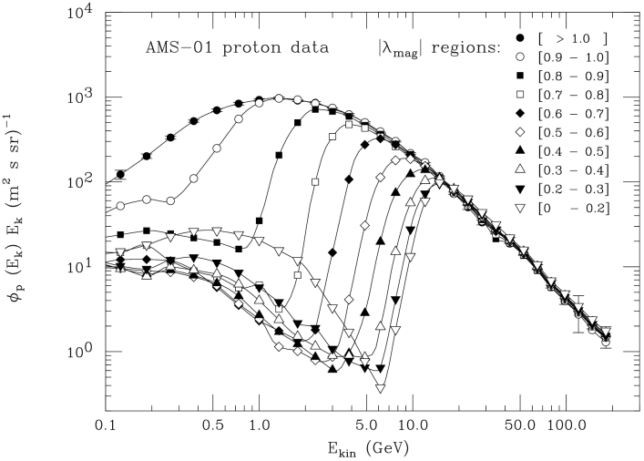
Figure 1: Cosmic ray proton flux measurements of the AMS detector [1] averaged for a detector position in ten regions of magnetic longitude. The error bars are shown only for one set of measures ($|\lambda_{{\rm mag}}|>1$ radiant). Note that for $E_{k}>0.3$ GeV the sub–cutoff proton flux is most intense in the magnetic equatorial region ($|\lambda_{{\rm mag}}|<0.2$).

The Anti Matter Spectrometer (AMS) collaboration has recently published the results on new measurements of the fluxes of cosmic ray protons [1], electrons and positrons [2] and Helium [3] performed during a ten days flight (STS–91) of the space shuttle in june 1998. These measurements have revealed the existence of significant fluxes of particles traveling on “forbidden trajectories”, that is with momenta below the calculated geomagnetic cutoff. These fluxes are refered to as “second spectra” in the AMS papers. Examples of the energy distributions of $p$ measured by AMS are shown in fig. 1 and 2. The second spectra fluxes exhibit a number of striking properties:

1. The ratio ³He/⁴He is of order $\sim 10$, two order of magnitude larger than the ratio found in the primary flux.

2. The ratio $e^{+}/e^{-}$ is of order $\sim 4$, to be compared with a ratio $\sim 0.10$ for the primary fluxes.

3. The past and future trajectory of each observed second spectrum particle can be calculated integrating the classical equations of motion of a charged particle in a detailed map of the geomagnetic field. All second–spectra particles appear to have origin in the Earth’s atmosphere, and to have trajectories that end in the atmosphere. The calculated flight time between the estimated origin and absorption points has a broad distribution extending from $\sim 10^{-2}$ to $\sim 10$ seconds. This time is much shorter than the typical confinement time of particles in the radiation belts, however the higher end of this range is also much longer than the Earth radius ($R_{\oplus}/c\simeq 0.021$ sec).

4. Two different “classes” of particles with different properties are seen: “short” and “long–lived” particles, depending on the calculated time of flight ($t$ greater or smaller than $\sim 0.3$ seconds). Long lived particles account for most ($\sim 70$% for $p$) of the second spectra fluxes.

5. Long lived particles appear to originate only from some well defined regions of the Earth’s surface that are different and well separated for particles of different electric charge. For example, positively charged particles ($p$, $e^{+}$ and Helium) detected in the magnetic equatorial region appear to have their origin from points in the same range of magnetic latitude but with longitude confined in the approximate interval: $\varphi\in[120^{\circ},300^{\circ}]$. On the contrary the calculated points of origin of $e^{-}$ have longitude in the complementary interval $\varphi\in[-60^{\circ},120^{\circ}]$. In the “allowed interval” of longitude the distributions of the creation points have a non trivial structure. For example most long lived positively charged particles originate from the longitude sub–intervals $\varphi\in[120^{\circ},180^{\circ}]$ and $\varphi\in[220^{\circ},280^{\circ}]$.

6. Similarly the absorption points of the long lived particles are confined to well defined regions, that are well separated for positively and negatively charged particles. The “sink” regions for positively charged particles approximately coincide with the “source” regions of negatively charged particles and viceversa.

7. For “short lived” particles the positions of the estimated origin and absorption points do not exhibit the interesting patterns described above.

8. The $e^{+}/e^{-}$ ratio is $\sim 4$ for long–lived and $\sim 2$ for short–lived particles.

9. The intensity of the second spectra fluxes is large. For protons in the magnetic equatorial region $|\lambda_{{\rm mag}}|<0.2$ ($\lambda_{{\rm mag}}$ is the magnetic latitude) it is of order $\sim 70$ (40) in units (m² s sr)^-1 for $E_{\rm kin}>0.1$ (0.3) GeV. This is comparable with the intensity of the primary $p$ flux reaching the equatorial region (of order $\sim 100$ in the same units).

The natural candidate mechanism as the source of the second spectrum particles is the production of secondary particles in the showers generated by cosmic rays in the atmosphere. A fraction of these secondary particles, produced with up–going directions, or bent into up–going directions by the geomagnetic field can in fact reach high altitude. These secondary particles have been known in the literature as the components of the “cosmic ray albedo” [4] (see also [5] for a recent measurement in a balloon experiment and additional references). In this work we will show that the simple hypothesis that the cosmic ray albedo is the source of the observed proton second–spectra is in good qualitative and quantitative agreement with the AMS data. This conclusion has also been reached by Derome et al. [6]. We will also discuss that all the “striking” properties of the second–spectra discovered by AMS have simple explanations in terms of the “albedo model”, and while not predicted, can be simply and naturally understood a posteriori.

This work has been also motivated by the importance of a detailed understanding of the cosmic ray (c.r.) fluxes for the calculation of the atmospheric neutrino fluxes. Recent measurements of these fluxes by the Kamiokande [7], IMB [8], Super–Kamiokande [9], MACRO [10] and Soudan–2 [11] detectors have given evidence for the existence of neutrino oscillations (or possibly some other form of new physics beyond the standard model [12]). The strongest evidence [9] comes from the observation of the suppression of the up–going $\nu_{\mu}$ and $\overline{\nu}_{\mu}$ fluxes with respect to the down–going ones. This can be interpreted as the “disappearance” of a fraction of the $\nu_{\mu}$ ($\overline{\nu}_{\mu}$) that travel long distances (comparable to the Earth radius) and transform into $\nu_{\tau}$ ($\overline{\nu}_{\tau}$) that are nearly “invisible” because most of them have energy below the threshold for $\tau$ production. Down–going neutrinos are produced by c.r. striking the Earth’s atmosphere near the detector position, while up–going neutrinos are produced in showers generated by c.r. above a much larger region of the Earth in the opposite hemisphere. It is clear that to reach the conclusion that $\nu$ oscillations are present (or in more detail to estimate how many neutrinos “disappear” or change flavor) one needs to know with sufficient precision the relative intensity of the cosmic rays fluxes striking the atmosphere over different positions on the Earth. Geomagnetic effects are important in determining then intensity and angular distribution of the c.r. fluxes that reach the Earth atmosphere, and have to be described correctly. To test the correctness of the treatment of these effects the AMS results are clearly of great value. In fact, because of the inclination of the space shuttle orbit during flight STS-91 (51.7^∘ with respect to the equator) and the Earth’s rotation, the AMS detector has measured, essentially simultaneously, the cosmic ray fluxes over a a large fraction ($\sim 89$%) of the Earth’s surface.

The calculations of the atmospheric neutrino fluxes, that have been used in the interpretation of the data [13, 14, 15], have assumed that the fluxes of c.r. particles below the geomagnetic cutoff are exactly vanishing. The new measurement tell us that this is an incorrect assumption, since the forbidden trajectories are populated by second–spectra particles. It is therefore necessary to investigate the possible impact on these sub–cutoff particles on the predicted intensity and angular distributions of the neutrinos fluxes.

Our conclusions are that the AMS results give an important confirmation of the assumption (of crucial importance for the neutrino flux calculations) that the cosmic ray flux in interplanetary space, when it is not disturbed by the geomagnetic effects, is isotropic. Furthermore the AMS data tell us that the description of geomagnetic effects used in recent calculations of the atmospheric neutrino fluxes [13, 14] are correct. The observed fluxes of sub–cutoff particles represent a neglibly small correction ($\sim 0.1\%$) to the neutrino event rates.

This work is organized as follows: in the next section we will discuss a montecarlo calculation of the proton albedo fluxes and compare the results with the AMS data; in section 3 we discuss the results, and illustrate how the observed properties of the albedo (or second–spectra) fluxes can be understood with simple qualitative arguments independently from a detailed calculation; section 4 discusses the impact of the albedo fluxes on the estimates of the atmospheric $\nu$ fluxes. The last section gives a summary and some conclusions. In an appendix we briefly present some general and well known results about geomagnetic effects that are used in this work.

2 Montecarlo calculation

In this section we will discuss a preliminary montecarlo calculation of the fluxes of “cosmic ray albedo” protons. In the following an “albedo” particle is a secondary particle produced by cosmic ray interactions in the atmosphere with a trajectory that reaches a minimum altitude $h\simeq 380$ Km (the approximate altitude of the space shuttle during flight STS–91). This is a straightforward problem, that is essentially identical to a (three–dimensional) calculation of the atmospheric neutrino fluxes. The montecarlo code is in fact the same one used for the calculation of the atmospheric neutrino fluxes described in [16]. It can be described as follows:

1. An isotropic flux of primary cosmic rays (protons and heavier nuclei) is generated “at the top of the atmosphere” (a surface with altitude $h=100$ Km).

2. To take into account of the geomagnetic effects, the past trajectory of each particle is studied, and particles on forbidden trajectories are rejected (see the discussion in A.3 in the appendix). The region with altitude $h>100$ Km is considered as “vacuum” except for the presence of a static magnetic field described by the IGRF model [17].

3. Each primary particle is then “forward” traced in the “atmosphere” (that is the region with $h<100$ Km) taking into account the presence of the magnetic field, and a variable air density (described as the average standard US atmosphere). An interaction point is randomly chosen, taking into account the cross section value and the variable air density. A few primary particles ($\sim 3$%) cross again the injection surface ($h=100$ Km) without interacting and are discarded.

4. The trajectories of all secondary protons with kinetic energy $E_{k}>300$ MeV (that is above threshold for $\pi$ production) produced in a primary interaction have been calculated integrating the equation of motion in a map of the geomagnetic field. Most secondary protons reinteract after traveling a short distance, however a few particles will reach high altitude. The only difference with the neutrino flux calculation [16] is that while in that work all stable particles that exited the “atmosphere” (that is the volume $h\leq 100$ Km) were discarded. These particles are now the the object under study, and their trajectories are calculated in detail, following the motion until they reaches a radius $r=10~{}R_{\oplus}$ (when the particle is considered as “free”), or interact in the atmosphere.

5. To estimate the flux associated with these “albedo” particles we have considered a “detector surface” at a constant altitude $h=380$ Km. Each time a proton crosses the detector surface (up–going or down–going) a “hit” is recorded, and a flux is estimated from the number of hits.

Some examples of trajectories of secondary particles that reach the altitude of the space shuttle orbit are seen in fig.3, 4, 5 and 6. A discussion of the properties of these trajectories will be made in the next section.

As an illustration of the calculation, in fig. 7 we show (with correct relative normalizations) the assumed energy spectra of primary protons in interplanetary space, the energy spectra of the protons that interact in the atmosphere in the equatorial region $|\sin\lambda_{\rm mag}|<0.4$, and the energy spectra of all secondary protons generated in the interactions in the same region. Comparing the first two histograms the effect of the geomagnetic field in suppressing the flux of primary low rigidity particles can be easily seen.

In fig. 8 we show (with correct relative normalization) the zenith angle distribution of all nucleons that interact in the magnetic equatorial region ($|\sin\lambda_{{\rm mag}}|<0.4$), the zenith angle of all nucleons that are the source of an albedo proton, and the zenith angle of albedo protons at the production point. As it is intuitive, quasi–horizontal trajectories, and “grazing” trajectories that do not intersect the surface of the Earth play an essential role as the source of albedo particles.

In fig. 9 we show (for the region $|\sin\lambda_{{\rm mag}}|<0.4$) the azimuth angle distribution of interacting nucleons, of the nucleons that are the source of albedo $p$, and of albedo protons at the production point. Most of the interacting primary particles are traveling toward the east. This is the well known east–west asymmetry [20, 21, 22], whose detection in the 1930’s allowed to determine that most c.r. have positive electric charge. The enhancement of the east–west effect for albedo particles is qualitatively easy to understand because the effect of the geomagnetic field on positively charged particles going east (west) is to bend them upward (downward) (see fig. 3 for an illustration).

In fig. 10 we show the the altitude distribution of the all nucleon first interaction points, and the altitude distribution of the production points of the albedo particles. As it is simple to understand, most albedo particles are created at high altitude.

The time $t$ associated to a computer run can be calculated as:

$$N_{p,{\rm gen}}=t~{}A_{\rm gen}~{}\pi~{}\int_{E_{\rm min}}^{\infty}dE~{}\phi_{p}(E)$$ (1)

where $N_{p,{\rm gen}}$ is the total number of primary proton simulated (including those rejected because of geomagnetic effects), $A_{\rm gen}=4\pi~{}R_{\rm gen}^{2}$ is the area over which the primary particles are generated, and $\phi_{p}(E)$ is the isotropic (interplanetary space) flux of primary protons.

Within the statistical uncertainties of the Montecarlo the upgoing and down–going fluxes of secondary particles are identical. To estimate the flux, because of the poor montecarlo statistics we have approximated the flux of albedo particle at the altitude of the AMS orbit as isotropic. For an isotropic flux $\Phi_{\rm iso}$ the rate of particle crossings a unit area detector surface is:

$$n_{\rm cross}=2\pi~{}\Phi_{\rm iso}~{}c\beta$$ (2)

where $\beta$ is the particle velocity and a factor of two takes into account up–going and down–going particles. We have then estimated the flux of albedo particles observable at the altitude of the AMS orbit as:

$$\Phi_{\rm albedo}={N_{\rm cross}\over 2\pi~{}c\beta\,t~{}A_{\rm det}}={1\over 2\,c\;\langle\beta\rangle}~{}{N_{\rm cross}\over N_{p,{\rm gen}}}~{}{A_{\rm gen}\over A_{\rm det}}~{}\Phi_{p,{\rm primary}}$$ (3)

where $N_{\rm cross}$ is the total number of recorded crossing of a “detector” surface of total area $A_{\rm det}$. For a “detector” over the region $|\lambda_{{\rm mag}}|<0.2$, the resulting flux is shown in fig. 11. In the same figure we also show the flux of vertical protons (selected in a cone of zenith angle $\theta<32^{\circ}$) averaged over all positions in the selected region. The result is compared with the AMS measurement in the same geographical region. The agreement is not perfect but reasonable, and the order of magnitude of the flux and qualitative features of the measurement are well reproduced.

In fig. 12 we show the distribution of the number of crossings that all “detected” particles. Particles with one crossing are in part ($\sim 40$%) protons produced with sufficiently high rigidity, so that they can escape to infinity never “returning” to the Earth’, and in part ($\sim 60$%) particles that that have a second (or more) crossings outside the selected equatorial region. The most probable situation for an albedo particle is to have two crossings. This corresponds to a proton that is generated in the atmosphere, goes to high altitude and returns close to the surface of the Earth where it is absorbed. We can see that there is also a significant probability of 4, 6, and more crossing, up to more than $10^{3}$ (an odd number of crossings correspond to a situation with at least one crossing outside the equatorial region).

The contribution of an albedo particle to the flux is proportional to the number of crossings of the detector surface. In fig. 13 we show an histogram of the relative contribution of particles with $N_{\rm cross}$ crossings to the estimated flux. One can see that albedo protons with long flight–paths even if they constitute a small fraction of the total number particles contribute most of the observed sub–cutoff flux.

In fig. 14 we show the positions of creation and absorption of “long–lived” particles (a flight time longer than 0.3 seconds, according to the definition of AMS). Histograms of the longitude distribution of the points is shown in fig. 15. The remarkable features of the distribution are in reasonable agreeement with the experimental results of AMS.

The results for the $p$ albedo fluxes in other regions of magnetic latitude have the same level of agreement with the AMS data.

3 Qualitative discussion

In this section we want to illustrate how all the most interesting features of the second spectra observed by AMS (listed in the introduction) can be naturally explained in the framework of a model where these spectra are composed of albedo particles.

3.1 Origin of the particles

A first remark is that when the past trajectories of the particles of the second spectra are calculated, it is found that all detected particles originate in the deep atmosphere. This result is not trivial. Second spectrum particles are by definition on forbidden trajectories, that is they do not come from “infinity”, however this does not a priori imply that their past trajectory will cross the Earth’s surface. In fact most trajectories of particles in the radiation belts [23] do not originate directly from the Earth’s atmosphere and have past trajectories that remain confined at high altitude. The creation point of these particles are inside the belt volume where the residual air density is very low, and for most particles the production mechanism is neutron decay. The second spectra on the other hand are produced inside the atmosphere, as cosmic ray albedo.

3.2 ³He/⁴He ratio

The very high ³He/⁴He ratio observed in the second spectrum is a very simple phenomenon to understand qualitatively. The key facts are that: (i) there is a large flux of primary ⁴He in the primary radiation; and (ii) that there is a large fragmentation cross section for the process ${}^{4}{\rm He}+{\cal A}\to{}^{3}{\rm Helium}+X$ (where ${\cal A}$ is an “air” nucleus) that accounts for $\sim 30\%$ of the inelastic cross section. Note that the presence of a fraction of $\sim 15\%$ of ³He in the primary radiation, much larger than the universal isotopic abundances, is the result of the fragmentation of a fraction of the accelerated Helium during propagation in the interstellar medium. In first approximation, in the fragmentation process the momentum per nucleon remain approximately unchanged. Therefore after the breaking–up process a ⁴He nucleus of momentum $p_{4}$ (and rigidity $R_{4}=p_{4}/2$) produces ³He fragments of momentum $p_{3}\sim{3\over 4}p_{4}$ and rigidity $R_{3}=p_{3}/Z\sim{3\over 4}~{}R_{4}$. The key result is that the rigidity of the ³He fragment is smaller that the rigidity of the projectile, and most ³He fragments produced by primary ⁴He with rigidity less that ${4\over 3}$ times the cutoff for the location and direction considered will be below cutoff and potentially trapped. A fraction of these fragments (especially those generated horizontal, east–going parents) will be injected into albedo particle trajectories.

In the fragmentation of a ⁴He nucleus, there are approximately equal probabilities to generate ³He and Tritium fragments (that can be considered as stable for the relevant short time scale of this problem). However this does not imply that the populations of the two nuclear species in the albedo spectra are approximately equal. Since a Tritium fragment has only one unit of electric charge, the relation between its rigidity and the rigidity of the primary ⁴He particle is $R_{T}\simeq{3\over 2}R_{4}$. In this case the fragment rigidity is larger than the primary particle one, and most Tritium fragments do not remain confined.

Helium–4 nuclei can be injected into trapped orbits when a primary ⁴He particle loses energy in an elastic scattering, or when a ⁴He fragment is produced in the interaction of heavier nuclei (such as ¹²C or ¹⁶O). These heavier nuclear species are less abundant than Helium in the primary flux, moreover since ⁴He and the most common heavier nuclei have the same $A/Z$ ratio, therefore the rigidity of an helium–4 fragment will be (most of the times) equal to the rigidity of the parent primary particle, that is above the geomagnetic cutoff. From these arguments one can reach the conclusion of a strong suppression for the injection of Helium–4 into trapped trajectories.

3.3 Positron/electron ratio in the albedo fluxes.

The qualitative reason for the high $e^{+}/e^{-}$ ratio observed in the subcutoff fluxes is illustrated in fig. 3 that shows a map of the Earth’s geographical equatorial plane with the calculated trajectories of four charged particles. Particle A is a primary proton with momentum $p_{A}=30$ GeV, that interacts at the point indicated by a small diamond, where it produced a secondary particle $a$ with positive unit charge and momentum $p_{a}=5$ GeV that crosses several times the altitude $h=380$ km, before being reabsorbed in the atmosphere. Both primary and secondary particle are east–going, and reversing the electric charge of $a$ would result in the immediate absorption of the particle. Particle B has also unit positive electric charge, and momentum $p_{B}=80$ GeV, and reaches the Earth atmosphere traveling on a west–going on a quasi–horizontal trajectory. At the interaction point a secondary particle $b$ with negative unit charge and momentum $p_{b}=4.5$ GeV is produced, that again is injected in a trajectory that crosses several times the altitude $h=380$ Km before being absorbed. Note that if a particle is west–going, it can be injected into the albedo flux only if it is negatively charged.

The figure illustrates three fundamental points:

1. albedo particles are most easily produced with initial zenith angle $\sim 90^{\circ}$ (approximately horizontally), and azimuth angle pointing east (for positively charged particles) and toward west (for negatively charged ones).

2. The directions of the primary and secondary particles are correlated because of momentum conservation.

3. The rate of east–going primary particles is larger than the rate of west going ones. The origin of this asymmetry (the celebrated east–west effect [20, 21, 22]) can be easily understood looking at fig. 3, where one can see that positively charged primary particles can reach the Earth equator from an horizontal west–going direction only if they have a gyroradius larger that $R_{\oplus}$ (this correspond to a rigidity $p/Z\buildrel>\over{{}_{\sim}}60$ GV), while the rigidity cutoff for east–going particles is much lower ($p/Z\buildrel>\over{{}_{\sim}}11$ GV).

Since the production of electrons and positrons in hadronic showers is approximately equal, it is now easy to reach the conclusion that the injection of albedo positrons, (mostly produced in the showers of nearly horizontal east–going primary particles) is significantly larger that the injection of electrons (mostly produced in the showers of less numerous west–going primary particles).

A remarkable property of the $e^{+}/e^{-}$ ratio measured by AMS [2], is the fact that the ratio for short lived ($e^{+}/e^{-}\sim 2$) and long lived ($e^{+}/e^{-}\sim 4$) particles differ by a factor of approximately two, with only a small energy dependence for $E\buildrel<\over{{}_{\sim}}1$ GeV. A qualitative explanation for this interesting phenomenon will be given in section 3.8.

3.4 The longitude distribution of the points of origin

The long lived positively charged particle observed in the magnetic equatorial region have their points of origin in the longitude range $\phi\in[120^{\circ},300^{\circ}]$ while negatively charged particles have their origin in the complementary longitude interval $\phi\in[-60^{\circ},120^{\circ}]$. This can be understood immediately on the basis of three simple observations.

1. Approximating the geomagnetic field as a dipole, one finds that the dipole is not only “tilted”, that is it with an axis not parallel to the Earth’s rotation axis, but is also “offset” that is the dipole center does not coincide with the Earth’s geometrical center.

2. The motion of charged particles confined to the equatorial plane of a magnetic dipole can be analysed as a “gyration” around a guiding center that drifts uniformly in longitude remaining at a constant distance from the dipole center (see fig. 6 and the discussion in A.4).

3. Positively charged particles drift westward (toward decreasing longitude) while negatively charged particles drift eastward (toward increasing longitude).

A scheme of the drift of particle in the equatorial plane of an offset dipole model is shown in fig. 18. It is simple to see that positively particles can be injected into albedo trajectories only if produced in one hemisphere, and are absorbed in the opposite hemisphere, while the opposite happens for negatively charged particles, since the longitude drift of the guiding center of the trajectory traveling at a constant distance from the dipole center has a variable altitude, that begins to decrease for particles created in the “forbidden” hemisphere, or to increase for particles created in the “allowed” one. The argument can be easily extended to the general case of of trapped trajectories, when the longitude drift is accompanied by an oscillation or “bouncing motion” along the field lines between symmetric mirror points. The altitude of the guiding center of the trajectory has minima (where the particle has the highest chance of being absorbed) at the mirror points that have a constant distance from the dipole center. In an offset dipole field the altitude of the mirror points change with the longitude drift. This mechanism can also be described in a more general, elegant and rigorous way making use of the concept of magnetic shells (see section A.7 in the appendix), and considering the intersections of the shells with the Earth’s surface.

For a description of the consequences of the dipole offset, it is convenient to “shift” the origin of the longitude defining:

$${\overline{\varphi}}=\varphi-\varphi^{*}$$ (4)

where $\varphi^{*}\simeq 120^{\circ}$ is the longitude of the dipole center seen from the Earth’s center (or also the longitude of the point of strongest field for a fixed latitude), and use the convention that the “shifted longitude” is defined in the interval $[-\pi,\pi]$. Then it is simple to see that the source and sink regions for positively and negatively particles are confined in longitude:

$$[{\rm Source}]_{+}\simeq[{\rm Sink}]_{-}\simeq\{{\overline{\varphi}}>0\}$$ (5)

$$[{\rm Source}]_{-}\simeq[{\rm Sink}]_{+}\simeq\{{\overline{\varphi}}<0\}$$ (6)

In the eccentric dipole model it is simple to predict an approximate one–to–one correspondence between the creation and absorption points of long–lived particles. An albedo positive particle created at longitude ${\overline{\varphi}}^{i}_{+}$ (with ${\overline{\varphi}}^{i}_{+}>0$) will be absorbed either “soon” or will drift for a “long” time clock–wise, that is toward decreasing $\varphi$. Let us consider for simplicity the motion of particles confined in the magnetic equatorial plane. During the drift the guiding center of the particle trajectory remains at a constant distance from the dipole center, therefore because of the dipole offset, the distance $r$ from the Earth center changes. For particles produced in the “allowed” longitude range $r$ starts increasing, and soon absorption in the atmosphere becomes impossible. The growth of the altitude of the trajectory guiding center will continue until the shifted longitude is ${\overline{\varphi}}\simeq 0$, then symmetrically it start to decrease. When the longitude becomes

$${\overline{\varphi}}^{f}_{+}\simeq-{\overline{\varphi}}^{i}_{+}$$ (7)

the particle will again be grazing the atmosphere, and will be reabsorbed. Symmetrically a negatively charged albedo particle created at a point ${\overline{\varphi}}^{i}_{-}<0$, will either be quickly absorbed or drift counter–clockwise until it reaches longitude

$${\overline{\varphi}}^{f}_{-}\simeq-{\overline{\varphi}}^{i}_{-}.$$ (8)

In both cases the total longitude drift is

$$\left|(\Delta\varphi)_{\rm drift}^{\pm}\right|\simeq 2\,|{\overline{\varphi}}_{i}^{\pm}|=2\,|{\overline{\varphi}}_{f}^{\pm}|$$ (9)

Note that particles produced with shifted longitude close to $|{\overline{\varphi}}|\simeq\pi$ drift for a longitude interval close to $2\pi$ that is nearly an entire Earth orbit, while particles with longitude close to ${\overline{\varphi}}\simeq 0$ will drift for a short distance.

This argument lead to the prediction of a simple relation between the time of flight of albedo particles, their position of creation and the momentum. The angular velocity of the drift motion was estimated in equation (23). Using that result we can deduce that for both positively and negatively charged particles:

$$t\simeq{|(\Delta\varphi)_{\rm drift}|\over\Omega_{\rm drift}}\simeq 1.8~{}{|{\overline{\varphi}}_{i}|\over\beta\,p({\rm GeV})}~{}{\rm sec}\simeq 1.8~{}{|{\overline{\varphi}}_{f}|\over\beta\,p({\rm GeV})}~{}{\rm sec}.$$ (10)

This is a remarkable relation between three quantities: the momentum of a second spectrum particle, its calculated time of flight, and the estimated longitude of the creation (or absorption) point. Any choice of a pair among these three quantities, allows to predict the third one. This relation is verified by the AMS data (see figure 6 in [2]).

A simple but important prediction of the “eccentric dipole model” is that it is difficult for a particle to perform an entire “drift” revolution around the Earth, as can be seen with simple geometrical considerations. This results in a simple prediction for the longest time of flight of albedo particles:

$$t_{\rm max}\simeq{2\pi\over\Omega_{\rm drift}}\simeq 5~{}{Z\over\beta\;p({\rm GeV})}~{}{\rm sec}.$$ (11)

3.5 Longitude dependence of the intensity of the albedo spectra

The AMS collaboration has presented its results on the cosmic ray spectra for different intervals in magnetic latitude for the detector position, integrating over the detector longitude. However, since the observation of the second spectra has given evidence of striking patterns in the longitude distribution of the creation points of the second spectra particles, it is natural to investigate the possible dependence of the flux intensity on the detector longitude. In the montecarlo study described in section 2, this dependence has been calculated (see fig. 16) obtaining a non trivial dependence.

For a qualitative understanding let us consider a a detector at a position with shifted longitude ${\overline{\varphi}}_{\rm det}$. From the results obtained in the previous subsection we can infer that when ${\overline{\varphi}}_{\rm det}>0$ the only observable long–lived particles are those produced in the longitude interval:

$${\overline{\varphi}}^{i}_{+}\in[{\overline{\varphi}}_{\rm det},\pi]$$ (12)

if positively charged, and

$${\overline{\varphi}}^{i}_{-}\in[-\pi,-{\overline{\varphi}}_{\rm det}]$$ (13)

if negatively charged. Note that the size of the two visible regions is :

$$|(\Delta{\overline{\varphi}})^{+}_{\rm visible}|=|(\Delta{\overline{\varphi}})^{-}_{\rm visible}|=\pi-|{\overline{\varphi}}_{\rm det}|$$ (14)

is equal for both positively and negatively charged particles, and strongly depends on the detector position, being maximum for a detector at ${\overline{\varphi}}_{\rm det}\simeq 0$, when the entire production regions of both positive and negative particles is visible, and vanishingly small for a detector at $|{\overline{\varphi}}_{\rm det}|\simeq\pi$.

This argument seems to imply that the intensity of the fluxes of long–lived albedo particles are linear in $|{\overline{\varphi}}_{\rm det}|$, however in this discussion we have not yet taken into account the altitude of the detector, that also plays an important role. The altitude of the guiding center of the trapped albedo particles also depend on the longitude, it is lowest at the creation and absorption points and it is highest at ${\overline{\varphi}}\simeq 0$. Therefore for a detector at a fixed altitude ($h\simeq 400$ Km in the case of AMS), only a fraction of the albedo flux will be visible, some part of it being too low and some part being too high.

The combination of these arguments: the “visible longitude horizon”, and the “altitude of the guiding center”, can explain the structure of the numerical results shown in fig. 16 that shows a minimum at the longitude $|{\overline{\varphi}}_{\rm det}|\simeq\pi$ (corresponding to $\varphi_{\rm det}\simeq 300^{\circ}$) and two maxima at longitudes 70^∘ and $150^{\circ}$, placed approximately symmetrically to the sides of the point ${\overline{\varphi}}_{\rm det}\simeq 0$. The gyroradius of the particles (see equation (19) is not negligiby small, and also plays an important role in determining which particles are “visible”. Therefore the longitude dependence of the flux, has different shapes for different momenta.

The range of longitude where we predict the lowest intensity of the albedo fluxes corresponds to the region closest to the south atlantic anomaly, where it is well known that the flux of trapped particles is extremely intense. This appears as a paradox, but it can be naturally explained. In fact the existence of the south atlantic anomaly and the patterns observed by AMS for the second spectra fluxes originate from the same cause, namely the offset of the dipolar component of the geomagnetic field. One consequence of the offset is that the “magnetic bottle” that contains charged particles in the inner Van Allen belt is not symmetric with respect to the Earth center. The south atlantic anomaly corresponds to the region where a tip of the “bottle” is closest to the Earth surface, descending to an altitude of few hundred kilometers over an area of South America and the south atlantic ocean, while on the other side of the Earth it remains above $\sim 1200$ Km. The existence of the “allowed” and “forbidden” hemisphere for the production of long lived albedo particles can be understood observing that the equatorial region of some magnetic shells (see section A.7) will intersect the Earth surface. Positive particles are created at one intersection between a magnetic shell and the Earth surface, and drift to be absorbed to the other interesection (and viceversa. for negatively charged particles). The particles are observable when the magnetic shell over which their guiding center is moving is close to the space shuttle orbit altitude. The longitude of the subatlantic anomaly, is roughly the longitude at which the equatorial region of the magnetic shells is closer to the Earth’s surface. It follows that when the detector is at the longitude of the anomaly, the observable flux of sub–cutoff particles is suppressed, since it is sitting on a shell that has no intersection with the atmosphere along its equatorial region.

3.6 Long lived and short lived particles

In the AMS papers the group makes a distinction about two classes of particles, “long–lived” and “short–lived”. The arguments presented above can be used to understand the existence and the properties of these two “classes” of particles.

The phenomenological evidence for the two clases of particles is perhaps most evident in fig. 6 of the paper [2] on subcutoff electrons and positrons. The figure shows a scatter plot of the time of flight of second–spectrum particles detected in the region $|\lambda_{{\rm mag}}|\leq 0.3$ versus their kinetic energy. Some interesting structures are immediately apparent:

1. There are two ‘horizontal bands’ that is particles with a time of flight $t\sim 0.03$ sec and $t\sim 0.06$ sec, and a wide range on energy.

2. There is a large “gap” in time of flight. For example there are few electrons or positrons with energy $E_{k}\simeq 0.3$ GeV and time of flight in the interval $t\in[0.09,2]$ seconds.

3. There are some broad “diagonal” bands. The two most evident bands (labeled as $A$ and $B$, in the AMS work [2]) are centered around the relations: $t\sim 1.5/p_{\rm GeV}$ sec and $t\sim 4/p_{\rm GeV}$ sec. The particles in each one of the bands originate in a well defined and distinct region of the Earth’s surface.

4. Finally no electrons or positrons have been detected with a time of flight longer than $t\sim 5/p({\rm GeV})$ sec

Particles in the “horizontal bands” are the “short lived” ones, particles in the “diagonal bands” are the “long–lived” ones. All these patterns have a simple qualitative explanation. The existence of the “horizontal bands” is due to the “bouncing” motion of trapped charged particles around the magnetic equatorial plane. As discussed in sec.A.2, the motion of a charged particle in a quasi–dipolar field can be decomposed into three components: a very fast gyration around a guiding center, a fast oscillation (or “bouncing”) around the magnetic equatorial plane, and a slow drift in longitude. The “bouncing period” of relativistic particles is momentum independent: $T_{\rm bounce}\sim 0.06/\beta$ sec (see equation (23) and the discussion in section A.4). Because of the structure of the field (see for example equation (18)), the altitude of the guiding center of a trapped trajectory is maximum on the equator and minimum at the “mirror points”. Particles are clearly created and absorbed near a mirror point.

The lowest “horizontal bands” in the flight–time versus momentum can be understood as due to particles that are never reflected, that is are produced in the northern (or southern) magnetic hemisphere and reabsorbed in the opposite one, after a single crossing of the magnetic equatorial plane. The next “horizontal band” is due to particles that perform one reflection, that is they are produced and absorbed in the same hemisphere after one reflection and two equatorial crossings.

While a particle “bounces” up and dow, in magnetic latitude, it is also drifting in longitude. The drift carries the altitude of the mirror points either lower (for positively charged particles with ${\overline{\varphi}}<0$ and negatively charged particles with ${\overline{\varphi}}>0$) leading to the particle absorption, or (in the complementary cases) higher. In the second situation, if the particle has not being absorbed after the first two reflections, it has a good chance to drift for a long time, until the altitude of the mirror points returns to roughly the initial level, at longitude ${\overline{\varphi}}_{f}=-{\overline{\varphi}}_{i}$. The existence of the “diagonal bands” is simply the consequence of equation (10); the bands are “diagonal” because the angular velocity of the longitude drift is $\Omega_{\rm drift}\propto p$ as discussed in section A.2.

In a “nutshell”: short lived particle are albedo particles that have only zero or one reflection at a mirror point. If a particle manages to have at least two reflections, and is produced in the “allowed” hemisphere for its electric charge, it has then a good chance to have a long trajectory with many bounces.

The argument that we have outlined here does not unexplain why there are well defined “bands” of particles, or in other words why the injection of particles in the long lived trajectories is more likely from some regions than from other ones. A qualitative explanation will be given in the next subsection.

3.7 Structure in the longitude distribution of the creation points

In the previous subsections, we have shown that a description of the geomagnetic field as a tilted and offset dipole is sufficient to understand qualitatively several important properties of the second spectra fluxes such as: (i) the existence of two rather well separated classes of “long” and “short” lived particles; (ii) the fact that long lived particles with positive or negative electric charge are produced in opposite hemispheres; (iii) the existence of a simple relation between the momentum, the longitude of the creation (or absorption) point and the time of flight of a long–lived “second spectrum” particle.

However the “eccentric dipole” description of the geomagnetic field predicts a smooth distributions for the longitude of the production and absorption points of the albedo particles. This is not supported by the data, that show that it is easy to produced albedo particles from some regions of the allowed hemisphere, and more difficult from others. In fact the longitude distribution of the second spectra particles clearly exhibits two maxima. These effects are reproduced with a Montecarlo calculation using a detailed map of the geomagnetic field (see fig. 15) that includes higher order terms in a multipole expansion. It is however instructive to understand qualitatively how the observed structures arise.

The argument that is perhaps most suitable for a qualitative understanding of the structure in the distribution in longitude of the production points, is based on a discussion of the “bouncing” motion of the trapped particles (see section A.2). Trapped charged particle trajectories in a dipole field can be analysed as a very fast “gyration” around a guiding center that moves oscillating along the field lines between symmetric mirror points, and drifting slowly in longitude. The same qualitative structure of the motion exists also for a non exactly dipolar field. The “bouncing” motion is possible only for sufficiently small amplitudes, so that both mirror points are at sufficiently high altitude. A necessary condition is obviously that they have radius $r>R_{\oplus}$. Note that since the drift frequency $\Omega_{\rm drift}$ is much smaller than the bouncing one $\Omega_{\rm bounce}$ (see equations (23) and (24)), it is a good approximation to study the bouncing motion neglecting the drift. In this way the guiding center of a particle trajectory can be seen as an oscillation along a particular field line. The center of the oscillation is the the point along the field line where the magnetic field is minimum (the “equator” point $E$ on the line), while the “mirror” points $M_{1}$ and $M_{2}$ have equal values of $|\vec{B}|$. The amplitude of the oscillation is in a one–to–one correspondence with the pitch angle of the particle at the point $E$. For a particle that at the minimum field (or equator) point is orthogonal to the field (that is has pitch angle $\cos\alpha_{0}\simeq 0$) the amplitude of the oscillation vanishes, with increasing $|\cos\alpha_{0}|$ the amplitude of the oscillation grows. The condition that the mirror points are above ground can be written (see the discussion in section A.5) as:

$$|\cos\alpha_{0}|\leq{\rm min}\left[\sqrt{1-{B_{\rm min}\over B(G_{1})}},\sqrt{1-{B_{\rm min}\over B(G_{2})}}\right]$$ (15)

where $B_{\rm min}$ is the minimum field along the line and $G_{1}$ and $G_{2}$ are the points of intersection of the field line with the ground.

For a centered dipole field the minimum field point coincides with the point of highest $r$ along a line and is symmetrically placed between the “ground” points $G_{1}$ and $G_{2}$, but this is not true in the general case. As an illustration in fig. 19 we show (in two separate panels) two geomagnetic field lines calculated using the IGRF 2000 field. The two lines have been selected so that the maximum altitude along the line is 150 Km (the maximum altitude point is labeled $A$), with longitudes $\varphi\simeq-140^{\circ}$ and $\varphi\simeq 170^{\circ}$ (this defines uniquely each field line). On each field line we have also indicated the point $E$ where the field has the minimum value. It is simple to see that if the point $E$ (the center of the oscillations) is displaced with respect to the geometrical center of the line, the maximum amplitude of the oscillations is reduced, and so is the range of possible pitch angles of trapped particles. Note also that if the “equator” point $E$ ha $r<R_{\oplus}$ a complete oscillation is impossible.

Let us now consider all field lines that have the point of maximum altitude at a fixed altitude $h$. A particular line in this set can be identified uniquely by the longitude of this point. For each line we can calculate using equation (15) the allowed range of pitch angles. The allowed interval of $\cos\alpha_{0}$ is proportional to the solid angle available for the injection of long lived albedo particles from the region in the atmosphere close to the “ground” points of the field line, that is the cone of initial directions, for which an albedo particle will be able to complete an entire latitude oscillations, and enter a “long” trajectory. The result of the calculation for the value $h=50$ Km is shown in the top panel of fig. 20. The height of 50 Km was chosen as a representative value for the field lines that are most important for the injection of particles in the albedo spectra from the magnetic equatorial region. This value is of course somewhat arbitrary, but the qualitative features of the figure are independent the precise value $h$. It can be seen that the allowed range in pitch angle for the different field lines exhibits some clear features:

1. There is a range of longitudes where oscillations are completely forbidden. In this region the equator point is below sea level.

2. There are two additional minima one in the region ${\overline{\varphi}}>0$ and one in the region ${\overline{\varphi}}<0$.

In the botton panel of fig. 20 we have multiplied the allowed range of pitch angle by the longitude drift of long lived particles created at that longitude (equation (9)). Particles with longer drifts give a larger contribution to the observed sub–cutoff flux. The features shown in fig. 20 reproduce qualitatively the structures observed in the data.

3.8 $e^{+}/e^{-}$ ratio for short and long lived particles

The discussion of the previous section can be used to obtain a qualitative understanding of the observed difference in the $e^{+}/e^{-}$ ratio for short–lived and long–lived particles. For short-lived particles (most of which are reflected only zero or one time in their “bouncing” motion) the enhancement of the positive partices can be understood as a consequence of (i) the larger flux of east–going primary particles over west–going ones, (ii) the correlation in direction between secondary and primary particles, and (iii) the fact that only positively (negatively) charged particles produced with east (west) going directions can be injected into the albedo fluxes. The same argument is of course valid also for long lived particles, however in this case we must also consider two conditions that are necessary for a particle to be “long lived”:

1. the particle must be created in the “allowed hemisphere”,

2. the particle must be able to complete a “bouncing” oscillations, that is it must be generated in an allowed cone of directions, that corresponds to an allowed range of pitch angles.

As discussed before, if a particle produced in the “allowed” hemisphere manages to perform one complete oscillation (two reflections), it is then likely to make many more, since the longitude drift “raises” the altitude of the mirror points.

In the previous subsection we have estimated “phase space” available (that is the range of possible pitch angles) for the injection of long lived particles from the equatorial region as a function of the longitude. The results are shown in fig. 20. From the figure it can be seen that the allowed solid angle for the longitude interval ${\overline{\varphi}}<0$ ($\varphi\simeq[-60^{\circ},120^{\circ}]$) that is the source of long lived negatively charged particles is significantly smaller than the allowed range in the complementary interval (the source of positively charged particles). This constitutes an additional suppression factor for negatively charged long lived particles that has to be combined with the effects due to east–west asymmetry if the primary flux. The results is a larger $e^{+}/e^{-}$ ratio for long lived particles, in agreement with the observations.

4 Implications for atmospheric neutrinos

To estimate the possible importance of the c.r. albedo fluxes for atmospheric neutrinos, it is useful to convolute the measured sub–cutoff fluxes at the space shuttle orbit with an “event yield” for $\nu$ charged current interactions. For example, for $\mu$ events the yield is defined as:

$$Y_{\mu}(E_{p})=N_{A}~{}\int dE_{\nu}~{}\left[{dn_{p\to\nu_{\mu}}\over dE_{\nu}}(E_{\nu},E_{p})~{}\sigma_{\nu_{\mu}}(E_{\nu})+{dn_{p\to\overline{\nu}_{\mu}}\over dE_{\nu}}(E_{\nu},E_{p})~{}\sigma_{\overline{\nu}_{\mu}}(E_{\nu})\right]$$ (16)

where $dn_{p\to\nu_{\mu}}/dE_{\nu}$ and $dn_{p\to\overline{\nu}_{\mu}}/dE_{\nu}$ are the average number of $\nu_{\mu}$ and $\overline{\nu}_{\mu}$ with energy $E_{\nu}$ produced in the shower of a proton of energy $E_{p}$, $\sigma_{\nu_{\mu}}$ and $\sigma_{\overline{\nu}_{\mu}}$ are the cross sections for $\nu_{\mu}$ and $\overline{\nu}_{\mu}$ charged current interactions [26] and $N_{A}$ is Avogadro’s number. In principle the $\nu$ event yield depends not only on the energy of the primary particle, but also on its zenith angle, since decay of mesons and muons (that are the $\nu$ sources) are more probable in inclined showers (see for example [16]); however for low $E_{p}$ this dependence is neglibly small, since all secondary products have low momentum, and unstable particles, because of their short decay lengths ($\ell_{\rm dec}=c\tau\,p/m$) decay rapidly with unit probability. A calculation of the yield for muon events estimated using the hadronic interaction model of the Bartol model [13] is shown in fig. 21. The yield vanishes for $E_{k}\buildrel<\over{{}_{\sim}}290$ MeV that is the threshold for $\pi^{\pm}$ (and therefore $\nu$) production and then grows rapidly with increasing energy.

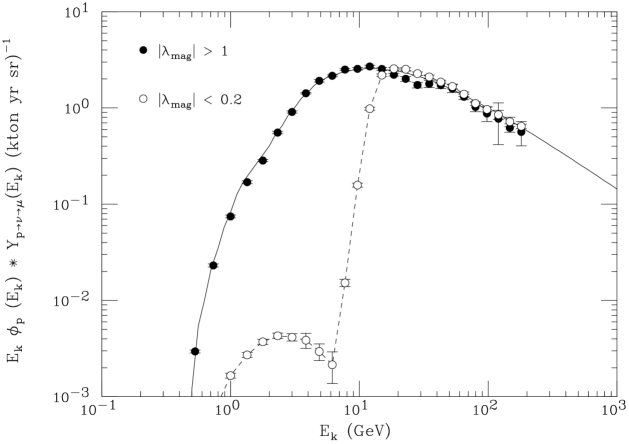
Figure 22: Convolution of the neutrino event yield for vertical protons with the fluxes observed at high altitude by the AMS detector in two regions of geomagnetic latitude.

The convolution of the Bartol $\nu$ event yield with the AMS proton–flux measured at high and low magnetic latitudes is shown in fig. 22. The integral of this convolution is $\sim 8.4$ (kton yr sr)^-1, for the high magnetic latitude region and $\sim 5.7$ (kton yr sr)^-1 for the magnetic equatorial region. The difference between the two rates represents the maximum possible size of geomagnetic effects. In the equatorial region the contribution due to second spectrum protons, obtained integrating for $E_{k}<6$ GeV, is $\simeq 0.009$ (kton yr sr)^-1, that is 0.16% of the total. The smallness of the contribution of the sub–cutoff particles to the $\nu$ rate, is a consequence of their softness. In the region considered, at the altitude of the space shuttle orbit, the sub–cutoff protons represent $\sim 42\%$ of the particle flux, but only $\sim 1.8\%$ of the energy flux, moreover only 60% of the second spectrum is above the kinematical threshold for $\nu$ production, and the $\nu$ that are produced are soft with low cross section.

The integration over solid angle of the effect is non trivial, however we can observe (see fig. 1 and 2) that the albedo spectrum has maximum intensity in the magnetic equatorial region, therefore simply multiplying by $4\pi$ we are making a conservative overestimate. The result is a contribution of second spectrum protons to the $\mu$–like event rate of 0.11 ($\mu$ events)/(kton year), that is of order 0.1% of a measured rate of $\sim 100$ events/(kton year).

This estimate, while already negligibly small, represents an overestimate of the effect. In fact the albedo flux that is observed at high altitude is enhanced because of the magnetic trapping. To estimate a correction factor to pass from the flux observed at high altitude to the flux that is absorbed in the atmosphere and is relevant for the production of secondary particles (such as neutrinos), we can use the results of the montecarlo calculation described in section 2, studying the average number of crossing of the “detector surface” (at the altitude $h=380$ Km) for all albedo particles that contribute to the flux at high altitude. In the region $|\lambda_{{\rm mag}}|<0.2$ this average number is $\langle n_{c}\rangle\sim 20$ for $E_{k}>0.3$ GeV, and $\langle n_{c}\rangle\sim 14$ for $E_{k}>1$ GeV. The energy dependence of $\langle n_{c}\rangle$ reflects the faster longitude drift of high momentum particles. Since each particle contributing to the albedo flux will interact a single time in the atmosphere, the quantity $\langle n_{c}\rangle^{-1}$ is a good estimate of the suppression factor.

This discussion can be summarized as follows. When the primary cosmic rays interact in the atmosphere, a small fraction of the incident energy flux “rebounds” in the form of outgoing “albedo particles”. Charged particles below the magnetic cutoff remain trapped in the geomagnetic field and populate the “second–spectra” observed at the space shuttle orbit. Eventually these charged particles are reabsorbed in the atmosphere, with peculiar angular and spatial (interaction point) distributions. The proton component of the second spectra produces neutrinos with a qualitatively estimated event rate of order 10^-2 events/(kton year), that is neglibly small when compared with the observed rate ($\sim 100$ in the same units). This small rate can be qualitatively understood observing that: (i) only $\sim 1\%$ of all showers produce an albedo proton, (ii) the fraction of the incident c.r. energy flux transformed into albedo protons is of order $\sim 10^{-3}$, (iii) the $\nu$ event yield of low energy $p$ is suppressed by kinematical effects.

5 Conclusions

In this work we have analysed the origin of the sub–cutoff spectra of cosmic rays measured at an altitude of $\sim 400$ km by the AMS detector. The natural source mechanism for these fluxes is the production of secondary particles in the atmosphere, injected into trajectories that reach high altitude as “albedo particles”. This simplest hypothesis allows to naturally explain the remarkable qualitative features of these subcutoff fluxes, such as the high ³He/⁴He and $e^{+}/e^{-}$ ratios, the separation into short and long lived particles, and the restrictions in the extension of the source and sink regions. We have performed a straightforward calculation of the $p$ flux, that requires less computer power than the calculation of the $e^{\pm}$ fluxes. In the calcuation we have used a rather crude model for the production of nucleons in the backward hemisphere of a c.r. interactions. Notwithstanding this limitation we obtain a reasonably good agreement with the AMS data, confirming the results of Derome et al [6].

The long time of flight of many particles in the sub–cutoff fluxes, is a consequence of the structure of the geomagnetic field. Because of the shape of the $L$ magnetic shells, or in less sophisticated language, because of the offset of the dominant dipolar component of the field with respect to the Earth center, the trajectory of the trapped particles generated close to the surface can remain for a long time at high altitude, with a guiding center, that oscillates in latitude, and drifts in longitude for as much as close to one complete revolution around the Earth. Also all the other “striking” properties of the sub–cutoff particles can be given simple, qualitative explanations.

The correct description of the cosmic ray fluxes reaching then Earth is important for the interpretation of the atmospheric neutrino data, that are giving evidence for the existence of new physics beyond the standard model. In this respect the existence if the subcutoff fluxes appears to be potentially important, especially because they exhibit striking patterns in the spatial distributions of their points of origin and absorption. A quantitative analysis however reveals that the contribution to the neutrino event rates of nucleon parents that enter the $p$ “second spectrum”, is a fraction below 0.1% of the observed rate, and is therefore negligible.

On the other hand the data of AMS, allow to test experimentally, some important elements in the calculation of the atmospheric neutrino fluxes: (i) the hypothesis of the isotropy of interplanetary space cosmic rays for the large angular scales relevant for atmospheric neutrino studies, and (ii) the reliability of the modeling of geomagnetic effects to determine which trajectories are allowed and which ones are forbidden. No significant deviations from the expectations have been detected, setting the best direct experimental constraints on these issues. Note that the study of the second spectra fluxes, are an excellent test of the quality of our description of geomagnetic effects, since to obtain agreement with the data one needs an accurate description of the field and of particle propagation in the field.

A detailed understanding of the fluxes of charged particles in near Earth orbit is important also as a input to the calculation of backgrounds for scientific instruments aboard satellites like for example the planned AGILE and GLAST high energy $\gamma$–astronomy telescopes. A work on this topic is in preparation [29].

It is interesting to consider the relation between the fluxes of sub–cutoff particles observed at the altitude of the space shuttle orbit and the fluxes of trapped particles in the radiation belts. In our view, a conceptual distinction between the two populations, can be tentatively made as follows: in one case (“second spectra” fluxes) the position of origin of a particle (and also its expected position of absorption when the particle is detected non destructively) can be estimated rather reliably and is close to the surface of the Earth where the atmosphere is dense; while in the second case (radiation belts particles) the trajectory treated as a classical trajectory in a static magnetic field has no “origin” and no “end” if energy loss mechanisms are neglected. The second case is possible because in a quasi–dipolar magnetic field there are many trapped trajectories that remain for an infinite amount of time (both in the past and in the future) in the space bound by two finite radii $r_{\rm min}$ and $r_{\rm max}$.

In the first case the injection of the particles in the population is “direct”, in the sense that they are generated either at the primary particle interaction point or “not too far”, in the subsequent shower. The “classical” definition of the “cosmic ray albedo” correspond closely to this concept of a population of secondary particles produced in cosmic rays showers, that can reach high altitude, even if perhaps not all properties of the albedo particles have been clearly understood. For example the distinction commonly made in the literature [4] between an upgoing “splash albedo” and a down–going “reentrant albedo”, has sometimes been interpreted as having the implication that “spash albedo” particles are generated in the vicinity of (below) the detector, and “reentrant albedo” particles are produced at the point of opposite (magnetic) latitude and approximately same longitude. It is indeed true that most albedo particles are never “reflected” by the magnetic field, and are reabsorbed at approximately the same longitude, however also in the light of the AMS results one must understand that albedo particles can “bounce” also many times between mirror points in the northern and southern hemisphere, with a long drift in longitude.

The mechanism considered as the main source of the charged particles trapped in the radiation belts, has been the decay of secondary neutrons [23]. Since the $n$ lifetime is long, the $n$ decay point (that is the creation point of a particle in the belt) is only weakly correlated with a c.r. shower.

As a final comment, I would like to speculate, that a significant source of particles in the inner belt could be related to the existence of populations of long lived albedo particles ($p$ and $e^{\pm}$) produced at intermediate magnetic latitudes. These particles have a confinement volume with similar shape to the inner belt (see for example figure 4 and 5), and can be the source of “permanently” confined lower rigidity particles via their interactions with the residual atmosphere at very high altitude.

Acknowledgments I have to express my gratitude to J. Arafune, T.Gaisser, M.Honda, T.Kajita, J. Nishimura and S.Vernetto for useful discussions. I’m also grateful to the R. Battiston, Yu. Galaktionov, E. Fiandrini, B. Bertucci and G. Lamanna for discussions about the AMS data. Finally my thanks to S. Ting for an invitation to the AMS workshop in the Ettore Majorana Center in Erice.

Appendix: Geomagnetic effects

A.1 The Earth’s magnetic field

It is well known that the Earth’s magnetic field to a first approximation can be described as a dipole field. In spherical coordinates the components of the field are:

$$B_{r}=-{M\over r^{3}}~{}2\,\sin\lambda;~{}~{}~{}~{}~{}~{}~{}~{}~{}B_{\lambda}={M\over r^{3}}~{}\cos\lambda.$$ (17)

where $M$ is the magnetic dipole moment and $\lambda$ is the magnetic latitude. For the Earth $M\simeq 8.1\times 10^{25}$ Gauss cm³, that corresponds to an equatorial magnetic field at the surface. $B_{\rm eq}\simeq M/R_{\oplus}^{3}\simeq 0.31$ Gauss. The field lines for a dipolar field have the form:

$$r=r_{0}~{}\cos^{2}\lambda$$ (18)

The module of the field $|\vec{B}|$ along each field line has its mimimum value on the equatorial plane ($\lambda=0$) at the point with the largest distance from dipole center (with $r=r_{0}$).

It is well known that the geomagnetic field is significantly different from the exact dipolar form. These deviations of the field from the dipolar form are essential for an understanding of the properties of the sub–cutoff fluxes. The sources of the magnetic field can be very naturally divided into “internal sources” (electric currents inside the Earth), and “external sources” (electric currents in space). The contribution to the field of the external sources exhibits variations also with very short (hours) time scale, connected with the position and magnetic activity of the sun, while the contribution of the “internal sources” varies only on much longer time scales, with a secular drifts of the magnetic poles. The magnetic field due to the external sources is the dominant contribution to $B$ at a distance of several Earth’s radii, but represent only a small perturbation in the vicinity of the Earth and will be neglected in this work, where the geomagnetic field will be described as in the International Geomagnetic Reference Field (IGRF) model [17] that is an empirical representation based on a multipole expansion. The coefficients of the different multipole terms (often called the Gauss coefficients) are slowly time dependent. In the numerical work we have used the IGRF field that corresponds to the 1st of january 2000.

It has been known for a long time, that if one wants to describe the geomagnetic field with a simple dipole, one obtains a significantly better fit with a dipole that is not only “rotated” with respect to the Earth axis, but it is also “offset” that is it has an origin that does not coincide with the Earth’s center. In the (standard) expansion of the field used in the IGRF model the origin of all multipole terms is the Earth’s center, however it is possible to approximately “reabsorb” the quadrupole contributions redefining the dipole moment and the position of its center. There is no unique well defined way to perform this redefinition of the dipole and different algorithms have been used for different applications. Qualitatively however the effect is quite clear. The dipole offset (planet center to dipole center) for the Earth is of order $\sim 450$ km and a vector from the Earth’s center to the dipole center has a latitude $\sim 18^{\circ}$ and a longitude $\varphi_{\rm dipole}\sim 140^{\circ}$. The approximate offset of the dipole axis with respect to the Earth’s center is of crucial importance for the understanding of the second spectra observed by AMS and is illustrated in fig. 17.

A.2 Motion of charged particles in a magnetic field

The properties of trajectories of charged particles in a magnetic field are a classic subject with a rich literature (see for example [24] for an elementary introduction, or [25] for a more detailed discussion). Here we will only recall some simple results that will be used in this work.

In a static homogeneous magnetic field the motion of a charged particle is a helix, with gyroradius $a$:

$$a({\rm Km})=33.3~{}{p_{\perp}({\rm GeV})\over B({\rm Gauss})}$$ (19)

This motion can be analysed as the combination of a rotation in a plane orthogonal to the field lines, accompanied by a uniform motion along the field lines.

In a non uniform static magnetic field where the distance scale $L$ of the field variation $L\sim|B^{-1}\partial B/\partial x_{j}|^{-1}$ is much larger than the gyroradius $a$ ($L\gg a$), the motion of a charged particle can again be decomposed as the rotation in a plane orthogonal to the field lines around a point (the “guiding center”) that has a motion both along and across the field lines. The motion parallel to the field lines is controlled by the variation of the field intensity along the field line. This behaviour can be deduced from the (adiabatic) conservation of the magnetic flux ($\pi a^{2}B$) through a particle’s circular orbit. The conservation of the magnetic flux can be written in the form:

$$v_{\perp}^{2}=v_{\perp 0}^{2}\;{B\over B_{0}}$$ (20)

Using the fact that $v_{\parallel}^{2}+v_{\perp}^{2}$ is constant, one can deduce the equation

$${\partial v_{\parallel}\over\partial\ell}\simeq-{v_{\perp 0}^{2}\over 2\,B_{0}}~{}{\partial B(\ell)\over\partial\ell}$$ (21)

($\ell$ is the distance along the field line) that describe the motion parallel to the field line. The increase of $B$ along the field line has a “repulsive effect” and is at the basis of the “magnetic mirror” effect.

When the gradient of the field has a non vanishing component $\nabla_{\perp}B\neq 0$, or when the field lines are curved, the guiding center has also a “drift” motion orthogonal to the field. Positively and negatively charged particles drift in opposite directions.

A.3 “Allowed”and “Forbidden” Trajectories

The fluxes of cosmic rays observed at points with different magnetic latitudes, are dramatically different, with the flux measured close to the magnetic equator strongly suppressed with respect to the flux measured at high magnetic latitudes. The discovery of the “latitude effect” [18, 19], lead to the understanding that the “cosmic radiation” was mostly composed of charged particles. Soon Bruno Rossi [20] observed that the geomagnetic effects should produce an east–west asymmetry, whose sign would determine if most c.r. are positively charged (excess of east–going particles) or negatively charged (excess of west–going particles). The effect was soon detected [21, 22], determining that most c.r. have positive electric charge.

The latitude and east–west effects are the simple consequence of the fact that low rigidity particles from outer space cannot reach the Earth’s surface because of the geomagnetic field. Let us consider a detector located at the position $\vec{x}$ that measures a particle of electric charge $Z$ and momentum $\vec{p}$. To a very good approximation the past trajectory of the detected particle can be determined integrating the classical equations of motion for a charged particle in an electromagnetic field in the region around the detector (and the Earth). Reconstructing this past trajectory there are three possible results:

• the trajectory originates from the Earth’s surface (or deep in the atmosphere);

• the trajectory remains confined in the volume $R_{\oplus}<r<\infty$ without ever reaching “infinity” (where $R_{\oplus}\simeq 6371.2$ Km is the Earth’s radius);

• the particle in the past was at very large distances from the Earth.

Trajectories belonging to the classes (a) and (b) are considered as “forbidden”, because no primary cosmic ray particle can reach the Earth from a large distance traveling along one of these trajectories. All other trajectories are allowed.

If we consider a fixed detection position $\vec{x}$ and a fixed direction $\hat{n}$, to a reasonably good approximation the trajectories of all positively charged particles with rigidity larger (smaller) than a cutoff $R_{+}^{\rm cutoff}(\vec{x},\hat{n})$ are allowed (forbidden). This is exactly true for a dipolar field that fills the entire space. In this case the solution (the “Störmer cutoff”) can be written down as an analytic expression [28, 16]. In the more general case it is necessary to study the problem numerically.

The effect of the geomagnetic field on an isotropic interplanetary flux is simply to “remove” the particles form the forbidden trajectories, without deforming the shape of the spectrum. This can be deduced from the Liouville theorem, with the assumption that the field is static [27].

A.4 Trapped particle trajectories in a dipole field

The motion of trapped particles in a dipolar magnetic field can be simply understood as the combination of three periodic motions having three very different characteristic frequencies. The first motion is simply the gyration around the magnetic field lines with a frequency

$$\Omega_{\rm gyro}={ZeB\over E}\simeq 9009~{}{Z\,B({\rm Gauss})\over E({\rm GeV})}~{}{\rm sec}^{-1}$$ (22)

The second component of the motion is a constant velocity longitude drift. Positive particle drift westward (toward decreasing longitude). Negative particles drift eastward (toward increasing longitude). The drift is simplest for particles that move in the equatorial plane. In this case it is elementary to show that the guiding center moves uniformly on a circle centered on the dipole with a frequency:

$$\Omega_{\rm drift}={3\over 2}~{}{r\over M}~{}\left({p\,\beta\over Ze}\right)\simeq 1.19~{}{r\over R_{\oplus}}~{}{p({\rm GeV})\,\beta\over Z}~{}{\rm sec}^{-1}$$ (23)

(for the numerical estimate we have used the Earth’s dipole moment). Note that the frequency is $\propto p$, and therefore the period to perform an orbit around the Earth is proportional to $p^{-1}$. This behaviour is easily understood qualitatively since the longitude drift is produced by the dishomogeneity of the field and the variations of the gyroradius of the particle as the particles moves. Higher momentum particles, with a larger gyroradius, are more sensitive to the gradient. Note also the curious result that the drift frequency is linear in $r$ that can also be understood considering the $r$ dependence of the field gradient.

The third component of the motion is an oscillation around the equatorial plane. A particle that finds itself on the equatorial plane with a non vanishing component of the momentum parallel to the field (that is with $\cos\alpha_{0}=0$, where $\alpha_{0}$ is the pitch angle on the equatorial plane) will bounce back and forth between (symmetric) maximum and minimum latitudes. The value of the field at the bouncing points is given by equation (20) solving for $v_{\parallel}=0$. It is clear that the amplitude of the oscillations is determined only by the pitch angle $\alpha_{0}$, and is independent from the particle momentum and electric charge. This latitude oscillation is to a good approximation an harmonic motion. For small amplitude oscillations (that is when the pitch angle in the equator plane $\alpha_{0}$ is close to $90^{\circ}$) the frequency is amplitude independent:

$$\Omega_{\rm bounce}^{0}={3\over\sqrt{2}}{\beta\over r}\simeq 99.8~{}\beta~{}{R_{\oplus}\over r_{0}}~{}{\rm sec}^{-1}$$ (24)

When the amplitude of the bounce increases (with growing $|\cos\alpha_{0}|$) the oscillation frequency depends weakly on the amplitude: $\Omega_{\rm bounce}(\cos\alpha)=\Omega_{\rm bounce}^{0}/\tau_{b}$ with $\tau_{b}$ a dimensionless quantity that is unity for $\cos\alpha_{0}=0$ and grows monotonically to $\tau_{b}\simeq 1.87$ for $\cos\alpha_{0}\to 1$.

A.5 “Bouncing motion”

It can be useful for the discussion to consider more closely the “bouncing” motion of the trapped particles, that is the oscillations of the guiding center of the particle trajectory between two mirror points placed symmetrically in the north and south hemisphere. It is obvious that only oscillations with a sufficiently small amplitude are possible, because following a field line, from a point $E$ in the equatorial plane (in either hemisphere) the radius $r$ decreases, and therefore if the amplitude of the oscillations are too large a particle “hits” the surface of the Earth and is absorbed.

The condition on the maximum amplitude can be translated in a (rigidity independent) condition on the pitch angle $\alpha_{0}$ of the trapped particles when they are on the equatorial plane. Let us consider the magnetic field line that passes through the point $E$ on magnetic equatorial plane. This line exits from the surface of the Earth in a point $G_{1}$ in the southern hemisphere, and reenters the Earth’s surface at a point $G_{2}$ (for a centered dipole the points $G_{1}$ and $G_{2}$ have the same magnetic longitude and symmetric latitudes: $\cos\lambda_{1,2}=\mp\sqrt{R_{\oplus}/r_{0}}$). The value of $|\vec{B}|$ along the field line has its mimimum at the point $E$ in the equatorial plane and grows monotonically with the distance from $E$ (symmetrically for a dipolar field). The increase of the field along the field line acts as “magnetic mirror” or repulsion (see equation (20)). A charged particle at the point $E$ with pitch angle $\alpha_{0}$ that is not exactly $90^{\circ}$, will have a component of momentum parallel to the field $p_{\parallel}=p\,\cos\alpha_{0}$ and will start moving along the field line, but the gradient of the field along the line will reduce and finally invert the parallel component. The inversion point is the “mirror” point. The component of the momentum parallel to the field at a point $P$ along the line ($\propto\cos\alpha$) depends of the value of the field at that particular point. From equation (20) one obtains:

$$\cos^{2}\alpha=1-\sin^{2}\alpha_{0}~{}{B\over B(E)}.$$ (25)

The mirror points ($M_{1}$ and $M_{2}$) are by definitions the points where the parallel momentum vanishes, that is:

$$0=1-\sin^{2}\alpha_{0}~{}{B(M_{1,2})\over B(E)}$$ (26)

The requirement that the two mirror points are above sea level can then be written as:

$$|\sin\alpha_{0}|\geq\left[{B(E)\over B(G_{1})}\right]^{{1\over 2}},~{}~{}~{}~{}~{}~{}~{}|\sin\alpha_{0}|\geq\left[{B(E)\over B(G_{2})}\right]^{{1\over 2}},$$ (27)

For a centered dipole field the two conditions in (27) are of course identical. Substituting the explicit expressions one obtains the condition:

$$|\sin\alpha_{0}|\geq r_{0}^{-{5\over 4}}\;(4r_{0}-3)^{-{1\over 4}}$$ (28)

(where $r_{0}$ is the radius of the equator point in units of $R_{\oplus}$). For example for an altitude of 100 Km equation (28) tells us that only particles with pitch angles between 75^∘ and 105^∘ can “bounce” without being absorbed by the Earth. When $r$ increases, larger amplitudes of the latitude oscillations become possible.

A.6 Examples of trajectories in the Earth’s field

For illustration in fig. 4,5 and 6 we show examples of trajectories of charged particles in the Earth’s field. These particles are examples of “long lived” particles generated as secondary protons in the interaction of cosmic ray protons in the atmosphere, and have a starting point in a point close to the Earth’surface where the density is large (at at an altitude of 40–50 Km above sea level). The trajectories have been calculated integrating numerically the classical equations of motion: $d\vec{p}/dt=e\vec{\beta}\wedge\vec{B}$ in the IGRF field. In each figure two panels show a {$X$,$Y$} (or equatorial) projection (that illustrate the longitude drift) and a {$\sqrt{X^{2}+Y^{2}}$,$Z$} projection (that illustrates the latitude bouncing). The coordinates are standard geographical coordinates.

The first example (fig. 4)) is a particle with momentum 2.31 GeV created at a latitude $\lambda\simeq-53^{\circ}$ in the southern hemisphere. In the {$\sqrt{X^{2}+Y^{2}}$,$Z$} projection it can be clearly that the particle spirals following the field lines, performing two “bounces”. The particle cannot perform one additional bounce because the bouncing point is “inside the Earth”, and the particle is absorbed. During the flight the particle drifts uniformly westard, as it is shown in the upper panel.

The trajectory of the particle in the example of fig. 5 was studied for a pathlength of $10^{6}$ Km, before interrupting the integration. In this case the particle performs many “bounces” and drifts in longitude for more than $2\pi$.

The third example in fig. 6, shows the trajectory of a particle that remains close to the equatorial plane of the field. It can be noted that the guiding center of the trajectory, travels in an approximately circular motion with a center that does not coincide with the Earth’s one. This is a consequence of the “offset” of the dipole component of the geomagnetic field.

A.7 Magnetic shells

The most powerful mathematical instrument to describe the motion of trapped particles in the Earth magnetic field is the concept of “magnetic shells”. This concept can be easily illustrated in the case of a dipole field. As discussed above, the motion of charged particles trapped in a dipole field can be regarded as the superposition of a circular motion in a plane perpendicular to the local magnetic field, around a “guiding center” that has a much slower motion. The“guiding center’ motion can be analysed as an oscillation along a guiding line that corresponds to a field line, and a still much slower rotation of the guiding line around the polar axis. The motion of the guiding center defines therefore a surface that can be called a “magnetic shell”. Each one of these shells corresponds to the surface generated by the rotation around the dipole axis of a field line. Explicitely, the magnetic shells have the form $r=r_{0}\,\cos^{2}\lambda$, and can be labeled with the parameter $r_{0}$. The set of the mirror points $M$ and $M^{*}$ (in the north and south hemispheres) where each individual particle “bounces”, that is inverts the direction of the motion along the field line, have a constant value of the magnetic field $B$.

In the real geomagnetic field the motion of trapped charged has qualitatively very much the same structure as in the dipole case. To a good approximation this motion can again be regarded as the superposition of a gyration and a motion of the guiding center. This last motion can again be analysed as an oscillation along a field line between mirror points that have a constant value of the magnetic field, and a slower drift in longitude. It can be demonstrated (see [25]) that if a charged particle starts oscillating along a particular field line, after drifting in longitude through 360^∘ it will return to the field line from which it started. Therefore the set of field lines along which a particle oscillate defines again a surface that closes upon itself as in the case of the dipole field. This surface can be again considered as a “magnetic shell” and is called an “$L$–shell”. The trajectory of the guiding center of particles that have latitude oscillations with different amplitudes, span different bands around the “equator” of the shell. In the case of a centered dipole field the $L$ parameter corresponds to the value $r_{0}/R_{\oplus}$; for an exact definition of the $L$ parameter in the general case see for example reference [25]. The magnetic field lines that belong to the same shell to a good approximation have the property that the minimum value of the field along the line is constant.

Disregarding the difference the positions of the particle and of its guiding center, the motion of a trapped charged particle are therefore confined to a well defined surface, that is the part of an appropriate magnetic shell, where the magnetic field is lower than a maximum value $B^{*}$ with the set of points on the shell where the field has the value $B^{*}$ corresponding to the set of mirror points for the particle trajectory. The set of all possible trajectories can be classified according to the two parameters ($L$ and $B^{*}$) that defines the shell, and the set of mirror points on the shell.

The magnetic shells of the real geomagnetic field are not exactly symmetric with respect to the Earth center. Qualitatively the most important feature is an offset, such that the equator of the most internal shells intersect the surface of the Earth. These intersection regions are both the source and sink regions of the long lived albedo particle. Since positively and negatively charged particles drift in opposite directions the sources of positive particles are the sink of negative particles and viceversa.

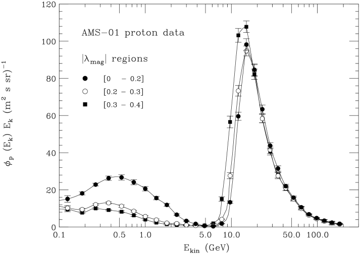
Figure 2: Cosmic ray proton flux measurements of AMS [1] averaged for a detector position in three regions of magnetic latitude.

Figure 3: The Earth’s equatorial plane with the projections of the trajectories of 4 particles with rigidities: $R_{A}=30$ GV, $R_{a}=5$ GV, $R_{B}=80$ GV and $R_{b}=-4.5$ GV. The diamonds indicate the final (starting) point of the trajectories for particles $A$ and $B$ ($a$ and $b$), these final (starting) points are on the equator, and have longitude $0^{\circ}$ and $90^{\circ}$ and altitude 20 Km. The dotted line indicates the altitude of the space shuttle orbit.

Figure 4: Example of the trajectory of a secondary proton in the geomagnetic field. Top panel: projection of the trajectory in the Earth’s equatorial plane. Bottom panel: projection in the plane $(\sqrt{X^{2}+Y^{2}},Z)$. (Geographical coordinates).

Figure 5: Example of the trajectory of a secondary proton in the geomagnetic field. This proton was traced for $10^{6}$ km without interactions in the atmosphere. Top panel: projection of the trajectory in the Earth’s equatorial plane. Bottom panel: projection in the plane $(\sqrt{X^{2}+Y^{2}},Z)$. (Geographical coordinates).

             

             

Figure 6: Trajectory in the geomagnetic field of a positively charged particle with rigidity 5.0 GV. The particle production point is near the equator, at an altitude of 50 Km and with an initial momentum pointing toward geographical east. Top panel: projection of the trajectory in the ($X$,$Y$) plane; bottom panel: projection in the ($\sqrt{X^{2}+Y^{2}}$,$Z$) plane.

Figure 7: The thin–solid line shows as a function of kinetic energy per nucleon the shape of the interplanetary nucleon spectrum assumed in the Montecarlo calculation. The thick histogram shows (with correct relative normalization) the energy distribution of all nucleons that interact in the Earth magnetic equatorial region $|\sin\lambda_{{\rm mag}}|<0.4$. The effects of the geomagnetic cutoff that “forbids” low rigidity trajectories are evident. The shoulder present at low energy is due to nucleons that reach the Earth in the form of bound nuclei, and that have higher rigidity for the same energy per nucleon (since $A/Z\simeq 2$). The thin histogram is the energy distribution of all secondary protons generated in the showers of the primary particles.

Figure 8: Dashed histogram: zenith angle distribution at the interaction point of all primary cosmic ray nucleons interacting in the Earth’s magnetic equatorial region $|\sin\lambda_{{\rm mag}}|\leq 0.4$ ($\cos\theta=-1$ corresponds to a vertically down–going particle). The histogram to a good approximation has the shape $\propto|\cos\theta|$, however few particles, bent by the geomagnetic field interact having an “up–going” direction. Thin–solid histogram: selection of nucleons that produced “albedo protons”, that is a secondary $p$ with a trajectory that reaches an altitude larger than 380 Km. Thick—solid histogram: zenith angle distribution at the production point of albedo $p$.

Figure 9: Azimuth angle distributions. Dashed histogram: primary cosmic rays at the interaction point; thin–solid histogram: primary particles that produce albedo $p$; thick–solid histogram, albedo $p$ at the creation point; thick–dotdashed histogram: long lived albedo $p$ ($t>0.3$ sec).

Figure 10: Thin histogram: distribution of the altitude of the interaction points of primary cosmic rays. Thick histogram: distribution of production points of albedo protons.

Figure 11: The data points are the measurements of the vertical proton flux by the AMS detector [1] in the region of magnetic longitude $|\lambda_{{\rm mag}}|<0.2$. The thin histogram is a montecarlo calculation of the primary vertical proton flux (averaged on 32^∘ cone) in the same region. The thick histogram is a montecarlo estimate of secondary protons reaching the altitude of 380 Km (always in the same region of magnetic latitude). The MC calculation was performed only for $E_{\rm kin}>0.290$ GeV

Figure 12: Dis tribution of the number of crossings that albedo particle have with a surface of constant altitude ($h=380$ Km) and magnetic latitude $|\lambda_{{\rm mag}}|\leq 0.3$.

Figure 13: Relative contribution of particles with $N_{\rm crossings}$ to the $p$ flux in the magnetic equatorial region ($|\lambda_{{\rm mag}}|\leq 11^{\circ}$) at an altitude $h=390$ Km.

Figure 14: In the top panel the dots represent the points of origin of long–lived albedo protons. In the bottom panel the dots represent the absorption points of long–lived albedo protons.

Figure 15: Histogram of the longitude of the production points of long–lived albedo protons detected in the magnetic equatorial region ($|\lambda_{{\rm mag}}|\leq 11^{\circ}$).

Figure 16: Longitude dependence of the $p$ albedo flux in the region $|\lambda_{{\rm mag}}|<0.2$ for $h=380$ Km and $E_{k}>0.3$ GeV.

Figure 17: The figure shows the magnetic equatorial plane of the Earth. The dipole axis is defined according to the first three terms of the IGRF expansion. The thick circle shows the surface of the Earth, the dashed lines are meridian lines, and the diamond indicates the position of the Greenwich observatory. The thin solid lines are line of constant field. It can be seen that the lines in first approximation are circles centered not on the Earth’s center, but on a point with $r/R_{\oplus}\sim 0.06$ and azimuth $\phi\sim 120^{\circ}$.

Figure 18: Illustration of the properties of the particle trajectories confined in the equatorial plane of an offset dipole model. The thick circle represents the intersection of the Earth’s surface with the dipole equatorial plane. Both the Earth’s center (point $O$) and the dipole center (point $D$) are on this plane. The thin circles represent the trajectories of the guiding center of the charged particles orbits. These trajectories remain at a constant distance $r_{\rm dip}$ from the dipole center, and therefore have a variable distance $r$ from the Earth’s center. Positively charged particles produced at the points $a$ and $c$ will drift westward and be reabsorbed at points $b$ and $d$. Negatively charged particles drift in the opposite (eastward) direction, therefore if produced at the points $a$ and $c$ will be rapidly reabsorbed, while if produced at the points $b$ or $d$ can have a long flight time reaching points $a$ and $b$.

Figure 19: Drawing of two field lines of the geomagnetic field. The point labeled with $A$ in the top (bottom panel) has altitude $h=150$ Km and longitude of $-140^{\circ}$ (170^∘). In both cases they are the points with highest $h$ along their field line. The points labeled as $E$ are the points on each line where the magnetic field has its minimum value. The field line intersect the Earth’s surface at the points labeled $G_{1}$ and $G_{2}$.

Figure 20: The top panel shows the quantity $\sqrt{1-B_{\rm min}/B(G)}$ for all field lines that have maximum altitude $h=50$ Km. Where $B_{\rm min}$ is the minimum value of the field along the line, and $B(G)$ is the minimum between $B(G_{1})$ and $B(G_{2})$ the field values at the two intersection points of a field line with the Earth’s surface. This corresponds to the maximum possible value of $|\cos\alpha_{0}|$ for particles that can oscillate along the line without hitting the Earth’s surface. The angle $\alpha_{0}$ is the pitch angle of the particle at the minimum field point $E$. The field lines are identified by the longitude of the equator point. The vertical dot–dashed lines separate the longitude regions for the injection of positive and negative particles. The vertical dotted lines separate regions labeled $A$ and $B$ in the AMS analysis [2]. The bottom panel shows the product $|\cos\alpha_{0}|_{\rm max}\times|\Delta\varphi_{\rm drift}|$ where $|\Delta\varphi_{\rm drift}|$ is the longitude drift of a charged particle injected into a “long” trajectory from a point with longitude $\varphi$ (equation (9)).

Figure 21: The points show the calculated yield of $\nu$–induced $\mu$–like events for vertical primary protons. The yield was calculated using Bartol shower model [13] and integrating over all $\nu$ production directions.