Quintessence dissipative superattractor cosmology

Abstract

We investigate the simplest quintessence dissipative dark matter attractor cosmology characterized by a constant quintessence baryotropic index and a power–law expansion. We show a class of accelerated coincidence–solving attractor solutions converging to this asymptotic behavior. Despite its simplicity, such a “superattractor” regime provides a model of the recent universe that also exhibits an excellent fit to supernovae luminosity observations and no age conflict. Our best fit gives $\alpha=1.71\pm 0.29$ for the power-law exponent. We calculate for this regime the evolution of density and entropy perturbations.

PACS number(s): 98.80.Hw, 04.20Jb

I Introduction

A new picture of the universe is emerging from observations of large scale structure, searches for Type Ia supernovae, and measurements of the cosmic microwave background anisotropy. They all suggest that the universe is undergoing cosmic acceleration and is dominated by a smoothly distributed dark energy component with large negative pressure [1, 2, 3]. Moreover, recent data coming from BOOMERANG and MAXIMA projects seem to indicate that the density of the universe is near the critical density [4]. The most frequently proposed candidates for this dark energy are a cosmological constant, or vacuum energy density [5], and quintessence [6], a scalar field with negative pressure. On the other hand, gravitationally clustered matter is usually assumed to be dominated by cold, collisionless, nonbaryonic dark matter (CDM).

In addition to the old cosmological constant problem, related to the smallness of the observational upper bound on the vacuum energy density compared to particle physics scales [7], a new challenge to the model with cosmological constant and CDM ($\Lambda$CDM) is the “cosmic coincidence” problem: why is it that the vacuum density dominates the universe only recently [8]. A dynamical self–interacting scalar field may explain why the dark energy is small. However, a minimally coupled scalar field combined with perfect fluid matter, such as in “tracking” QCDM models [9], cannot explain the observed acceleration and solve the coincidence problem [10, 11]. On the other hand it has been shown in Ref. [10] that both acceleration and coincidence can be satisfactorily explained by a combination of quintessence and dissipative dark matter (QDDM). For these models it was shown that late–time attractor solutions exist with very interesting properties: an accelerated expansion, spatially flatness, and a fixed ratio of quintessence to dark matter energy density. Recently, it has been shown that such accelerated coincidence–solving attractor solutions also exist in spatially flat models with an exponential self-interaction quintessence potential and phenomenologically chosen couplings between the quintessence field and baryotropic dark matter [12, 13].

Consideration of dissipative effects in dark matter also arises from increasing evidence that numerical simulations of dark matter halos on sub-galactic scales based on conventional CDM models lead to conflicts with observations. One of the major problems shown by these simulations is that galactic halos are too centrally concentrated [14]. Confirmation of this problem would imply that structure formation is somehow suppressed on small scales. Several scenarios addressing this issue have been considered assuming some kind of interaction for dark matter particles: nonthermally produced and weakly interacting [15], self–interacting [16], repulsive [17], annihilating [18], and decaying [19]. It is quite reasonable to expect that dark matter is out of thermodynamical equilibrium and these same interactions are at the origin of the cosmological dissipative pressure. A simple estimation shows that a cross section of the order of magnitude proposed in these halo formation scenarios, corresponding to a mean free path in the range $1$ kpc to $1$ Mpc, yields at cosmological densities a mean free path a bit lower than the Hubble distance. Hence a description for interacting dark matter as a dissipative fluid is valid at cosmological scales [20].

Dark matter may also have several components, from very heavy weakly interacting massive particles to a lightweight neutrino [21]. Even if this neutrino-like component does not contribute significantly to the density budget of the universe [3], it may have nevertheless a relevant dynamical role as distinct components of dark matter, cooling at different rates, give rise to bulk viscosity [22].

Recently the relationship between dark matter clustering, the nature of dark matter and the origin of ultrahigh energy cosmic rays (UHECRs) has been explored [23]. Heavy particles ($m_{X}\sim 10^{12}-10^{14}$ GeV) can be produced in the early universe in different ways [24, 25, 26, 27] and their lifetime can be finite though longer than the age of the universe. In these circumstances, super-heavy particles can represent an appreciable fraction of dark matter and the decay of these particles results in the production of UHECRs, as widely discussed in the literature [25, 28, 29, 30]. In particular, if the relics cluster in galactic halos, as is expected, they can explain the cosmic ray observations above $\sim 5\times 10^{19}$ eV. The effect of decaying dark matter on the equation of state has been studied numerically in Ref. [31], and the equivalence between particle production and dissipative bulk viscosity has been investigated in Ref. [32].

All this shows that many different scenarios may occur where significant dissipative processes develop in dark matter, in particular when it behaves as a viscous fluid. So a variety of accelerated coincidence–solving attractors are possible. In this paper we will show that for a wide class of QDDM models attractor solutions are themselves attracted towards a common asymptotic behavior, the “superattractor”. The superattractor scenario is described in Sec. II and observational constraints on this scenario are investigated in Sec. III. These include the luminosity distance–redshift relation for type Ia supernovae and the age of the universe. We apply the covariant gauge–invariant formalism to calculate the evolution of density and entropy scalar perturbations in the QDDM regime and solve them for the superattractor regime in Sec. IV. Finally the main conclusions are discussed in Sec. V. Units in which $c=8\pi G=k_{B}=1$ are used throughout.

II QDDM superattractor scenario

In Ref. [10] it was shown that the Friedmann–Lamaitre–Robertson–Walker (FLRW) universe filled with perfect normal matter plus quintessence fluid, corresponding to some minimally coupled scalar field governed by the Klein–Gordon equation, cannot at the same time drive an accelerated expansion and solve the coincidence problem. To solve it, some additional bulk dissipative pressure $\pi$ in the stress–energy tensor of dark matter was considered. Any dissipation in FLRW universes has to be scalar in nature, and in principle it may be modeled as a bulk viscosity effect within a nonequilibrium thermodynamic theory such as the Israel–Stewart theory [33, 34]. In a certain regime, that formulation can be approximated by the more manageable truncated transport equation

$$\pi+\tau\dot{\pi}=-3\zeta H\,,$$ (1)

where $H\equiv\dot{a}/a$ denotes the Hubble factor, $\zeta$ stands for the phenomenological coefficient of bulk viscosity, and $\tau$ is the relaxation time associated with the dissipative pressure [35, 36, 37]. As usual an overdot means derivative with respect to cosmic time.

The overall stress–energy tensor of the QDDM model reads

$$T_{ij}=(\rho_{m}+\rho_{\phi}+p_{m}+p_{\phi}+\pi)u_{i}u_{j}+(p_{m}+p_{\phi}+\pi)g_{ij},$$ (2)

where $\rho=\rho_{m}+\rho_{\phi}$ and $p=p_{m}+p_{\phi}$. Here $\rho_{m}$ and $p_{m}$ are the energy density and pressure of the matter whose equation of state is $p_{m}=(\gamma_{m}-1)\rho_{m}$ with baryotropic index in the interval $1\leq\gamma_{m}\leq 2$. Likewise $\rho_{\phi}$ and $p_{\phi}$, the energy density and pressure of the minimally coupled self–interacting quintessence field $\phi$, are related by the equation of state, $p_{\phi}=(\gamma_{\phi}-1)\rho_{\phi}$, with baryotropic index

$$\gamma_{\phi}=\frac{\dot{\phi}^{2}}{\dot{\phi}^{2}/2+V(\phi)},$$ (3)

where for non-negative potentials $V(\phi)$ one has $0\leq\gamma_{\phi}\leq 2$. The scalar field can be properly interpreted as quintessence provided $\gamma_{\phi}<1$ –see e.g. [6]. In general $\gamma_{\phi}$ varies as the universe expands, and the same is true for $\gamma_{m}$ since the massive and massless components of the matter fluid redshift at different rates.

The Friedmann equation and the energy conservation of the normal matter fluid and quintessence (Klein–Gordon equation) are

$$H^{2}+\frac{k}{a^{2}}=\frac{1}{3}(\rho_{m}+\rho_{\phi})\qquad(k=1,0,-1),$$ (4)

$$\dot{\rho_{m}}+3H\left(\gamma_{m}+\frac{\pi}{\rho_{m}}\right)\rho_{m}=0,$$ (5)

$$\dot{\rho_{\phi}}+3H\gamma_{\phi}\rho_{\phi}=0,$$ (6)

where the prime means derivative with respect to $\phi$. Introducing $\Omega_{m}\equiv\rho_{m}/\rho_{c}$, $\Omega_{\phi},\equiv\rho_{\phi}/\rho_{c}$, with $\rho_{c}\equiv 3H^{2}$ the critical density and $\Omega_{k}\equiv-k/(aH)^{2}$ plus the definition $\Omega\equiv\Omega_{m}+\Omega_{\phi}$, the set of equations (4)–(6) can be recast as (cf. [38])

$$\Omega_{m}+\Omega_{\phi}+\Omega_{k}=1,$$ (7)

$$\dot{\Omega}_{m}+3H\left(\gamma_{m}+\frac{\pi}{\rho_{m}}+\frac{2\dot{H}}{3H^{2}}\right)\Omega_{m}=0\,,$$ (8)

$$\dot{\Omega}_{\phi}+3H\left(\gamma_{\phi}+\frac{2\dot{H}}{3H^{2}}\right)\Omega_{\phi}=0\,,$$ (9)

where $\gamma$ is the effective baryotropic index given by

$$\gamma\Omega=\gamma_{m}\Omega_{m}+\gamma_{\phi}\Omega_{\phi}.$$ (10)

Equations (7)–(9) have fixed point solutions $\Omega=1$, $\Omega_{m}=\Omega_{ma}$ and $\Omega_{\phi}=\Omega_{\phi a}$, respectively, when the partial baryotropic indices and the dissipative pressure are related by

$$\gamma_{m}+\frac{\pi}{\rho_{m}}=\gamma_{\phi}=-\frac{2\dot{H}}{3H^{2}}.$$ (11)

Asymptotical stability of $\Omega=1$ occurs whenever $\gamma+\pi/\rho<2/3$. This condition, together with Eq. (11), leads to the additional constraints $\pi<\left(2/3-\gamma_{m}\right)\rho_{m}$, which is negative for ordinary matter fluids, and $\gamma_{\phi}<2/3$. Additionally the stability of $\Omega_{m}=\Omega_{ma}$ and $\Omega_{\phi}=\Omega_{\phi a}$, and hence of the ratio $\Omega_{m}/\Omega_{\phi}$, has been established in [10]. These solutions provide a natural explanation to several features observed in our universe: an accelerated expansion, spatial flatness, and a ratio of dark energy to matter density of order unity. We denote by a subindex $a$ the asymptotic limit of magnitudes in the attractor regime, while the subindex $0$ will denote as usual their current values.

Combining Eq. (11) with Eq. (1) we obtain the equation of motion of the attractor solutions of the system (4), (5), (6), (1) satisfying flatness, acceleration and coincidence:

$$\nu^{-1}\left(\frac{\ddot{H}}{H}+3\gamma_{m}\dot{H}\right)+\dot{H}+\frac{3\gamma_{m}}{2}H^{2}-\frac{3\zeta}{2\Omega_{ma}}H=0\,.$$ (12)

Here $\nu=\left(\tau H\right)^{-1}$ is the number of relaxation times in a Hubble time – for a quasistatic expansion $\nu$ is proportional to the number of particle interactions in a Hubble time. Perfect fluid behavior occurs in the limit $\nu\to\infty$, and a consistent hydrodynamical description of the fluids requires $\nu>1$. Rewriting (12) in terms of the field baryotropic index $\gamma_{\phi}$, we get

$$\gamma^{\prime}_{\phi}=3\gamma_{\phi}^{2}-(\nu+3\gamma_{m})\gamma_{\phi}+\nu\left(\gamma_{m}-\frac{\zeta}{\Omega_{ma}H}\right)\,,$$ (13)

where a prime indicates derivative with respect to $\eta=\ln a$.

When the phenomenological coefficient of bulk viscosity satisfies $\zeta=\zeta_{s}$, where

$$\zeta_{s}=\Omega_{ma}\left(\gamma_{m}-\gamma_{\phi s}\right)\left[1-3\gamma_{\phi s}\,\nu^{-1}\right]H\equiv\kappa H\,,$$ (14)

Eq. (13) admits the constant solution $\gamma_{\phi}=\gamma_{\phi s}$. It gives an accelerated expansion in the late time regime when $\gamma_{\phi s}<2/3$. As $\zeta>0$ and $\gamma_{m}\geq 1$, the hydrodynamical parameter $\nu$ is restricted to $\nu>3\gamma_{\phi s}$. The case of constant $\kappa$ in the interval $0<\kappa<1$ arises, for instance, in a radiating fluid, and the nearly linear regime, with slowly varying $\nu$ and $\gamma_{m}$, was already investigated in the quasiperfect limit, corresponding to $\nu^{-1}\to 0$ [10].

To analyze the stability of the solution $\gamma_{\phi}=\gamma_{\phi s}$ we insert Eq. (14) into (13)

$$\gamma^{\prime}_{\phi}=3\left(\gamma_{\phi}^{2}-\gamma_{\phi s}^{2}\right)-(\nu+3\gamma_{m})\left(\gamma_{\phi}-\gamma_{\phi s}\right)\,.$$ (15)

As $\gamma_{\phi s}<2/3$, $\nu>\mbox{\rm max}(3\gamma_{\phi s},1)$, and $\gamma_{m}\geq 1$, Eq. (15) shows that $\partial\gamma_{\phi}^{\prime}/\partial\gamma_{\phi}<0$ in a neighborhood of $\gamma_{\phi s}$. Hence this constant solution is asymptotically stable, showing that all solutions of Eq. (12), that is, all the accelerated coincidence–solving attractors of the system (4), (5), (6), (1), are themselves attracted towards the constant solution $\gamma_{\phi}=\gamma_{\phi s}$ provided that they satisfy $\zeta\sim\zeta_{s}$ when $t\to\infty$. As the same occurs with all solutions whose initial conditions lay within the domain of attraction of each of these attractor solutions, we will refer to the constant solution as the “superattractor” of this class of QDDM models. We denote with subindex $s$ magnitudes in the superattractor regime. As an example of models satisfying $\zeta\to\zeta_{s}$ we note the case $\zeta\propto\sqrt{\rho_{m}}$, investigated in Refs. [39, 40, 41, 42].

Let us characterize this asymptotic stage. From Eq. (11) the superattractor solution yields a power–law evolution for the scale factor

$$a_{s}(t)=a_{0}\left(\frac{t}{t_{s}}\right)^{\alpha}\,,$$ (16)

where $\alpha=2/3\gamma_{\phi s}$, $a_{0}$ is the current scale factor and $t_{s}$ is the age of a superattractor universe. The dynamics of the scalar field in the attractor regime is obtained from Eqs. (3) and (11):

$$V=\frac{3}{2}\Omega_{\phi a}(2-\gamma_{\phi})\,H^{2}\,,$$ (17)

$$\dot{\phi}^{2}=3\Omega_{\phi a}\gamma_{\phi}\,H^{2}\,.$$ (18)

These equations together with (12) close the problem of finding the potential $V$ and the scalar field $\phi$ as functions of $t$. Expressing the potential (17) and field (18) in terms of cosmological time, that is, $V=\Omega_{\phi a}(3H^{2}+\dot{H})$ and $\dot{\phi}^{2}=-2\Omega_{\phi a}\dot{H}$, it is easy to find, for the superattractor solution,

$$V_{s}(\phi)=\frac{2\Omega_{\phi a}}{3\left(\gamma_{\phi s}t_{s}\right)^{2}}(2-\gamma_{\phi s}){\mbox{e}}^{-A\phi}\,,$$ (19)

$$\phi_{s}(t)=\phi_{0}+\sqrt{\frac{4\Omega_{\phi a}}{3\gamma_{\phi s}}}\,\ln\frac{t}{t_{s}}\,,$$ (20)

where $A=(3\gamma_{\phi s}/\Omega_{\phi a})^{1/2}$ is the slope parameter. Then we find $\alpha=2/(\Omega_{\phi a}A^{2})$ and $\phi_{0}=(2/A)\ln\gamma_{\phi s}$. We note that in the superattractor regime, the exponent $\alpha$ is larger, by a factor of $1/\Omega_{\phi a}$, than the exponent $2/A^{2}$ of a scalar field dominated era. This is a particular instance of a general property of QDDM models in that dissipative effects assist quintessence driven acceleration through the negative non-equilibrium pressure $\pi$. Using Eq. (11) we can evaluate its ratio to quintessence pressure:

$$\frac{\pi}{p_{\phi}}=\frac{\gamma_{\phi}-\gamma_{m}}{\gamma_{\phi}-1}\frac{\Omega_{ma}}{\Omega_{\phi a}}\,.$$ (21)

Hence, in the superattractor regime, this ratio is also a constant (provided that $\gamma_{m}$ is a constant), and when dark matter is cold it is just the ratio of matter to quintessence energy density.

Let us sketch the evolution of the actual universe from a nearly thermodynamical equilibrium early era (when $\pi/\rho_{m}\simeq 0$) into this superattractor stage (when $\pi/\rho_{m}=\gamma_{\phi s}-\gamma_{m}$). Along the radiation and matter dominated eras $|\pi/\rho_{m}|\ll 1$ and the inequality $\gamma_{m}+\pi/\rho_{m}>\gamma_{\phi s}$ holds. Then dissipative processes become more significant, the attractor condition (11) is approached, $\gamma_{\phi}$ is driven towards $\gamma_{\phi s}$, and the expansion of the scale factor accelerates. Clearly the timescale of this transition period depends on the details of the dissipative processes occurring in dark matter, encoded into the evolution of the dissipative magnitudes $\zeta(t)$ and $\nu(t)$ – some models exhibiting this convergence stage have been investigated in Ref. [10]. The superattractor stage finally settles when $\zeta\simeq\zeta_{s}$. Assuming that the ratio of this transition period to the age of the universe $t_{0}$ is small and this transition period started early enough, we may approximate the recent evolution of $a(t)$ by the superattractor solution (16); hence, $\gamma_{\phi 0}\simeq\gamma_{\phi s}$ and $(1+z)^{-1}=a/a_{0}\simeq(t/t_{0})^{\alpha}$.

As Eq. (19) shows, the class of models converging to the superattractor stage has $V(\phi)\sim V_{s}(\phi)$ for large $\phi$. In addition to this exponential tail, no other constraint has to be imposed on the quintessence potential for convergence to the superattractor era. For a wide range of initial values of $\phi$ and $\dot{\phi}$ the quintessence field approaches a common evolutionary path (20) for which $\gamma_{\phi}=\gamma_{\phi s}$; i.e., the late behavior is insensitive to the initial conditions.

III Observational constraints

A Luminosity distance of supernovae

It has been found that supernovae of type Ia (SNeIa) are nearly standard candles. Properly corrected, the difference in their apparent magnitudes is only related to differences in luminosity distance $d_{L}$ and consequently to cosmological parameters [43, 44]. Taking profit of this property, several accelerated expanding cosmological models like $\Lambda$CDM and QCDM have been fitted to recent observations of high redshift supernovae ($z\mbox{\raisebox{-3.00003pt}{$\stackrel{{\scriptstyle<}}{{\sim}}$}}1$) [43, 45, 46, 47]. Though they have a good fit in some regions of the parameter space corresponding to an accelerated expansion, these models require fine tuning to account for the observed ratio between dark energy and clustered matter.

On the other hand, QDDM models provide models that simultaneously provide an accelerated expansion and solve the coincidence problem within the general trend of the universe towards an attractor and with it towards the superattractor. As in QCDM models, these scenarios depend on the quintessence potential and initial conditions. In addition, they depend on the evolution of the magnitudes characterizing the details of dissipative processes occurring in dark matter. Let us examine the issue of reconstructing part of this evolution through observations of distant SNeIa.

Ignoring gravitational lensing effects, the standard expression for the luminosity distance to an object at redshift $z$ in a spatially homogeneous and isotropic universe is [48]

$$d_{L}(z)=\frac{1+z}{H_{0}|\Omega_{k0}|^{1/2}~{}}{\cal S}\left(H_{0}|\Omega_{k0}|^{1/2}\int_{0}^{z}\frac{dz^{\prime}}{H(z^{\prime})}\right),$$ (22)

with ${\cal S}(u)=(\sin u,u,\sinh u)$ for $k=(1,0,-1)$ respectively. Then for a QDDM universe we have

$$\frac{H(z)}{H_{0}}=\left\{\Omega_{m0}\exp\left[{3\int^{z}_{0}\,\frac{dz^{\prime}}{1+z^{\prime}}\left(\gamma_{m}+\frac{\pi}{\rho_{m}}\right)}\right]\right.$$

$$\left.+\Omega_{\phi 0}\exp\left({3\int^{z}_{0}\,\frac{dz^{\prime}}{1+z^{\prime}}\,\gamma_{\phi}}\right)+\Omega_{k0}(1+z^{\prime})^{2}\right\}^{1/2}$$ (23)

In the case of a spatially flat universe, $d_{L}$ has a simpler expression in terms of the effective baryotropic index

$$d_{L}(z)=\frac{1+z}{H_{0}}\int^{z}_{0}dz^{\prime}\exp\left[-{\frac{3}{2}\int^{z^{\prime}}_{0}\,\frac{dz^{\prime\prime}}{1+z^{\prime\prime}}\left(\gamma+\frac{\pi}{\rho}\right)}\right]$$ (24)

where

$$\gamma+\frac{\pi}{\rho}=\gamma_{m}+\frac{\pi}{\rho_{m}}-\left(\gamma_{m}+\frac{\pi}{\rho_{m}}-\gamma_{\phi}\right)\Omega_{\phi 0}\exp\left({3\int^{z}_{0}\,\frac{dz^{\prime}}{1+z^{\prime}}\,\gamma_{\phi}}\right)$$ (25)

We see from Eqs. (24) and (25) that $d_{L}(z)$ depends on the time evolution of dissipative processes through a double integral in $\pi/\rho_{m}(z)$ and on the time evolution of the quintessence field through a double or triple integral in $\gamma_{\phi}(z)$ (we assume that $\gamma_{m}\simeq 1$). On one the hand, there is a degenerancy here as these two functions cannot be reconstructed from knowledge of the single function $d_{L}(z)$. Besides the time variation of these magnitudes is largely smoothed out and, similarly to the analysis in Refs. [49, 50, 51] for QCDM models, we find that the luminosity distance is highly insensitive to these variations. So we may safely replace these time-varying magnitudes by their mean values in the interval $(0,z)$. Assuming that the universe has already settled in the superattractor regime at the age of the farthest observed supernova the degenerancy is eliminated and both functions become constant. Then, the expression (24) simplifies drastically and we obtain (cf. [52])

$$d_{L}(z)=\frac{\left(1+z\right)\left[(1+z)^{\beta}-1\right]}{\beta H_{0}}\,,$$ (26)

where $\beta=a\ddot{a}/\dot{a}^{2}=1-1/\alpha$ is the acceleration parameter. So $\beta$ increases with $\alpha$ and $1<\alpha<\infty$ corresponds to $0<\beta<1$. On the superattractor we have

$$\gamma_{\phi s}={2\over 3\alpha}=\frac{2}{3}(1-\beta)\,.$$ (27)

We have used the sample of $38$ high redshift ($0.18\leq z\leq 0.83$) supernovae of Ref. [43], supplemented with $16$ low redshift ($z<0.1$) supernovae from the Calán/Tololo Supernova Survey [53]. This is described as the “primary fit” or fit C in Ref. [43], where, for each supernova, its redshift $z_{i}$, the corrected magnitude $m_{i}$ and its dispersion $\sigma_{i}$ were computed.

The predicted magnitude for an object at redshift $z$ with luminosity distance $d_{L}$ is

$$m(z)={\cal M}+5\log{\cal D}_{L}(z),$$ (28)

where ${\cal M}$ is related to the absolute magnitude $M$ by

$${\cal M}=M-5\log\left(\frac{H_{0}[\mbox{\rm km/s Mpc}]}{c[\mbox{\rm km/s}]}\right)+25$$ (29)

and ${\cal D}_{L}$ is the luminosity distance in units of the Hubble radius.

We have determined the optimum fit of the superattractor model by minimizing a $\chi^{2}$ function:

$$\chi^{2}=\sum^{N}_{i=1}\frac{\left[m_{i}-m(z_{i};\beta,{\cal M})\right]^{2}}{\sigma_{i}^{2}}\,,$$ (30)

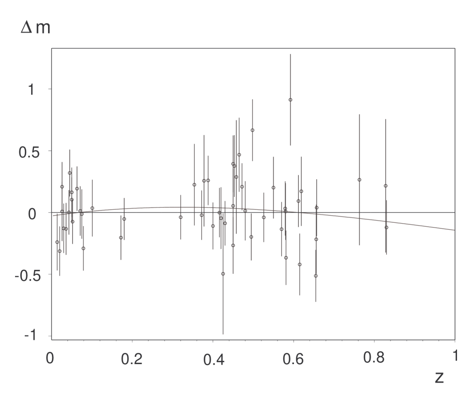
where $N=54$ for this data set. The most likely parameters are $(\beta,{\cal M})=(0.395,23.96)$, yielding $\chi^{2}_{min}/N_{DF}=1.12$ ($N_{DF}=52$), and a goodness–of–fit $P(\chi^{2}\geq\chi^{2}_{min})=0.253$. These numbers show that the fit of superattractor QDDM cosmology to this data set is as good as the fit of the $\Lambda$CDM model (see Fig. 1). We note that it occurs even though the superattractor model has basically only the acceleration parameter to fit large redshift supernovae (${\cal M}$ being largely determined by low redshift supernovae). It also means that the density of clustered matter is not constrained by measurements of SNeIa and it has to be determined through independent observations.

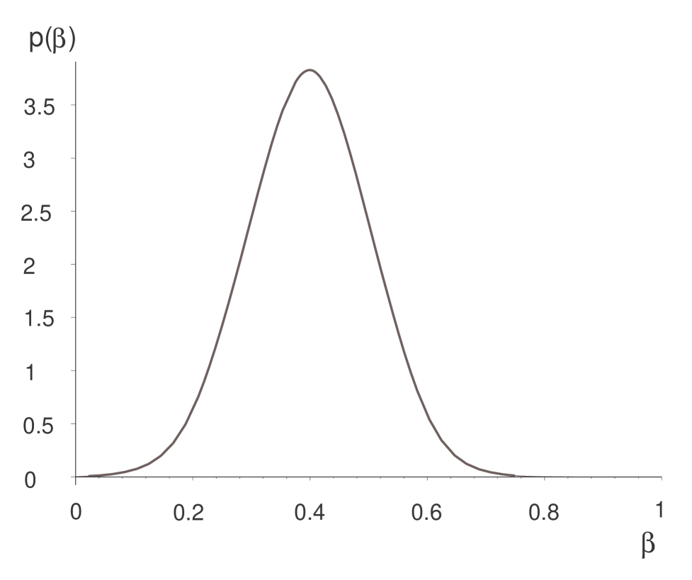
We estimate the probability density distribution of the parameters by evaluation of the normalized likelihood [54]

$$p(\beta,{\cal M})=\frac{\exp\left(-\chi^{2}/2\right)}{\int d\beta\int d{\cal M}\exp\left(-\chi^{2}/2\right)}\,.$$ (31)

Then we obtain the probability density distribution for $\beta$ marginalizing $p(\beta,{\cal M})$ over ${\cal M}$. This probability density distribution $p(\beta)$ is plotted in Fig. 2 and it yields $\beta=0.398\pm 0.104$ $(1\sigma)$. Hence we can state that $0.085<\beta<0.711$ with a confidence level of $0.997$, so that an accelerated superattractor QDDM universe is strongly supported by this data set, in agreement with a similar analysis of $\Lambda$CDM and QCDM models [43, 44, 55, 46].

B Age of the Universe

For a QDDM model the age of the universe has the integral representation

$$t_{0}=\int^{\infty}_{0}\frac{dz}{\left(1+z\right)H(z)}\,,$$ (32)

where $H(z)$ is given by Eq. (23). Along the transition period of the universe from an early nearly equilibrium stage towards the superattractor stage the inequality $\gamma_{m}+\pi/\rho_{m}>\gamma_{\phi s}$ holds. As a consequence $H(z)>H_{s}(z)=H_{0}(1+z)^{1-\beta}$ (whenever $\Omega_{k}\geq 0$) and $t_{0}<t_{s}=\alpha/H_{0}$. The characteristics of this transition period, and hence the value of the difference $t_{s}-t_{0}$, are model dependent and will not be dealt with here.

Using the fit to SNe Ia of the previous subsection and Eq. (27) we obtain $\alpha=1.711\pm 0.288$. Combined with $H_{0}=65\pm 5$ km/s Mpc [2], it yields for the age of the superattractor universe $t_{s}=25.9\pm 4.8$ Gyr. This shows that the QDDM cosmology does not suffer of any age discrepancy and can accommodate comfortably the $1\sigma$ interval $9$–$16$ Gyr for the age estimate of globular clusters [3].

C Parameters of the superattractor era

Using the probability distribution for $\beta$ and Eq. (27) we obtain $\gamma_{\phi s}=0.401\pm 0.069$, in agreement with previous results for QCDM models in the limit $\Omega_{m}\to 0$. Then, using Eq. (11) and assuming that dark matter is cold ($\gamma_{m}=1$), we find $\pi/\rho_{m}=-0.599\pm 0.069$. This figure implies that substantial dissipative processes are taking place in dark matter. This fact is also shown by the large value of the effective baryotropic index. In effect, combining the estimate $\Omega_{m0}=0.35\pm 0.07$ from cluster baryons [2] with the a priori constraint $\Omega=1$ and inserting into Eq. (10) we get $\gamma_{s}=0.61\pm 0.09$. For a perfect fluid this value would correspond to a power-law exponent $2/3\gamma_{s}\simeq 1.1$, quite lower than $\alpha$. Using Eq. (14), we find that the linear relationship $\kappa=\kappa_{1}+\kappa_{2}\nu^{-1}$ holds, where $\kappa_{1}=0.21\pm 0.05$ and $\kappa_{2}=-0.25\pm 0.07$. The requirement of asymptotic stability of the superattractor solution imposes that $\nu>1.20\pm 0.21$.

Using Eqs. (17) and (18), we find the quintessence kinetic energy density parameter $\Omega_{K0}=0.13\pm 0.03$ and $\Omega_{V0}=0.52\pm 0.06$ for the potential energy density parameter. These figures show that the scalar field is moving down the potential outside the slow–roll regime. Similarly we find for the slope of the exponential potential $A=1.36\pm 0.14$ and for the current value of the scalar field $\phi_{0}=-1.3\pm 0.3$. This implies a mass parameter of the Planck scale.

IV Density perturbations

Besides the model degenerancy of luminosity distance determinations, even within the superattractor cosmology there are some thermodynamical parameters like $\nu$ and the speed of sound $c_{\rm s}$ that are not fixed. For this reason we will investigate the evolution of density fluctuations in the perturbative long–wavelength regime during the superattractor era. It is possible that weak lensing techniques could yield more information about these parameters [56].

Scalar perturbations are covariantly and gauge–invariantly characterized by the spatial gradients of scalars. Density inhomogeneities are described by the comoving fractional density gradient [57]

$$\delta_{i}={\frac{a\mbox{D}_{i}\rho}{\rho}}\,,$$ (33)

where $\mbox{D}_{i}$ stands for the covariant spatial derivative $\mbox{D}_{j}A_{i\cdots}=h_{j}{}^{k}h_{i}{}^{l}\cdots\nabla_{k}A_{l\cdots}$. The scalar part $\delta\equiv a\mbox{D}^{i}\delta_{i}=(a\mbox{D})^{2}\rho/\rho$ corresponds to the usual gauge-invariant density perturbation scalar $\varepsilon_{\rm m}$ [58, 59], which encodes the total scalar contribution to density inhomogeneities. Also the comoving expansion gradient, the normalized pressure gradient, and normalized entropy gradient are defined by [57, 60]

$$\theta_{i}=a\mbox{D}_{i}\theta\,,\quad p_{i}={\frac{a\mbox{D}_{i}p}{\rho}}\,,\quad e_{i}={\frac{anT\mbox{D}_{i}s}{\rho}}\,,$$ (34)

$n$ being the particle number density, $T$ the temperature, and $s$ the specific entropy per particle. The evolution equation for scalar density perturbations reads [60]

$\displaystyle\ddot{\delta}+H\left(8-6\gamma+3c_{\rm s}^{2}\right)\dot{\delta}-{\textstyle{3\over 2}}H^{2}\left\{1+5\left(\gamma-1\right)^{2}-6c_{\rm s}^{2}+\right.$

$$\left.\left[(1-3\left(\gamma-1\right)^{2}+2c_{\rm s}^{2}\right]k\right\}\delta-c_{\rm s}^{2}\mbox{D}^{2}\delta={\sf S}[e]+{\sf S}[\pi]+{\sf S}[q]+{\sf S}[\sigma]\,,$$ (35)

where

$$c_{\rm s}^{2}=\left({\frac{\partial p}{\partial\rho}}\right)_{\!s}\,,\quad r={\frac{1}{nT}}\left(\frac{\partial p}{\partial s}\right)_{\!\rho},$$ (36)

are, respectively, the adiabatic speed of sound and a non-baryotropic index. The sources in the right–hand side of Eq. (35) arising, respectively, from entropy perturbations, bulk viscous stress, energy flux, and shear viscous stress are given in [60]. Since in our case there are no shear viscous stress ($\sigma_{ij}=0$) and ${\sf S}[q]$ vanishes by choosing the energy frame ($q_{i}=0$), we reproduce here only the expressions for ${\sf S}[e]$ and ${\sf S}[\pi]$:

$${\sf S}[e] = r\left(3kH^{2}+\mbox{D}^{2}\right)e\,,$$ (37)

$${\sf S}[\pi] = -\left(3kH^{2}+\mbox{D}^{2}\right){\cal B}\,,$$ (38)

where the scalar entropy perturbation

$$e=a\mbox{D}^{i}e_{i}={\frac{a^{2}nT}{\rho}}\mbox{D}^{2}s$$ (39)

and the dimensionless perturbation scalar

$${\cal B}={\frac{a^{2}\mbox{D}^{2}\pi}{\rho}}\,,~{}$$ (40)

related to the inhomogeneous part of the bulk viscous stress, were defined.

Also, the entropy perturbation equation in the energy frame is

$$\dot{e}+3H\left(c_{\rm s}^{2}-\gamma+1+r\right)e=-3H{\cal B}\ .$$ (41)

The coupled system that governs scalar dissipative perturbations in the general case is given by the density perturbation equation (35), the entropy perturbation equation (41), the equation for the scalar bulk viscosity (1), and the equation for temperature perturbations.

When only bulk viscous stress dissipation is present, the coupled system can be reduced to a pair of coupled equations in $\delta$ (third order in time) and $e$ (second order in time). For a flat background, the equations are [60]:

$\displaystyle\tau\stackrel{{\scriptstyle\ldots}}{{\delta}}+\left[1+3\left(2-\gamma+c_{\rm s}^{2}\right)\tau H\right]\ddot{\delta}+H\left\{8-6\gamma+3c_{\rm s}^{2}+3\tau\left(c_{\rm s}^{2}\right)^{\displaystyle{\cdot}}\right.$

$\displaystyle\left.-{\textstyle{1\over 2}}\left[-14+75\gamma-48\gamma^{2}+(21\gamma-30)c_{\rm s}^{2}\right]\tau H\right\}\dot{\delta}$

$\displaystyle-{\textstyle{3\over 2}}H^{2}\left\{6-10\gamma+5\gamma^{2}-6c_{\rm s}^{2}-4\tau\left(c_{\rm s}^{2}\right)^{\displaystyle{\cdot}}\right.$

$\displaystyle\left.-2\left[-6+18\gamma-15\gamma^{2}+5\gamma^{3}+\left(6-28\gamma+10\gamma^{2}\right)c_{\rm s}^{2}\right]\tau H\right\}\delta$

$\displaystyle={\frac{a^{2}\zeta}{\rho\gamma}}\mbox{D}^{2}\left(\mbox{D}^{2}\dot{\delta}\right)+{\frac{3a^{2}(\gamma-1)H}{\rho\gamma}}\mbox{D}^{2}\left(\mbox{D}^{2}\delta\right)+\tau c_{\rm s}^{2}\mbox{D}^{2}\dot{\delta}+\tau r\mbox{D}^{2}\dot{e}$

$\displaystyle+\left[\left(1-3\gamma\tau H\right)c_{\rm s}^{2}+\tau\left(c_{\rm s}^{2}\right)^{\displaystyle{\cdot}}+3\left({\frac{\partial\zeta}{\partial\rho}}\right)_{\!s}\right]\mbox{D}^{2}\delta$

$$+\left[\left(1-3\gamma\tau H\right)r+\tau\dot{r}+3\left({\frac{\partial\zeta}{\partial s}}\right)_{\!\rho}\right]\mbox{D}^{2}e\,,$$ (42)

and

$\displaystyle\tau\ddot{e}+\left[1-{\textstyle{3\over 2}}\left(-2+3\gamma-2c_{\rm s}^{2}-2r\right)\tau H\right]\dot{e}$

$\displaystyle-3H\left[\gamma-1-c_{\rm s}^{2}-r+3\gamma\left(\gamma-c_{\rm s}^{2}\right)\tau H+\tau\left(c_{\rm s}^{2}+r\right)^{\displaystyle{\cdot}}\right.$

$$\left.-{\frac{\rho}{\gamma}}\left({\frac{\partial\zeta}{\partial s}}\right)_{\!\rho}\right]e=-{\frac{\zeta}{\gamma}\ }\dot{\delta}+{\frac{3H}{\gamma}}\left[\left(\gamma-1\right)\zeta+\rho\left({\frac{\partial\zeta}{\partial\rho}}\right)_{\!s}\right]\delta\,.$$ (43)

We shall consider here the evolution of the density and entropy perturbations in the superattractor stage with the conditions $r=0$ and $\partial\nu/\partial s=0$. Together with Eq. (14) they imply

$$\left(\frac{\partial\zeta}{\partial s}\right)_{\rho} = 0\ ,$$ (44)

$$\left(\frac{\partial\zeta}{\partial\rho}\right)_{s} = \left(\frac{\partial\zeta}{\partial\rho_{m}}\right)_{s}=\frac{\kappa_{1}+\kappa_{2}/\nu}{6\Omega_{m}H}$$ (45)

In this case, Eq. (42) decouples to give

$$\stackrel{{\scriptstyle\ldots}}{{\delta}}+\frac{c_{1}}{t}\ddot{\delta}+\frac{c_{2}}{t^{2}}\dot{\delta}+\frac{c_{3}}{t^{3}}\delta = c_{4}\ t^{2\alpha}\ \mbox{D}^{4}\dot{\delta}+c_{5}\ t^{2\alpha}\ \mbox{D}^{4}\delta+c_{\rm s}^{2}\mbox{D}^{2}\dot{\delta}$$ (47)

$$+\left(\frac{c_{6}}{t}+c_{7}\right)\mbox{D}^{2}\delta\ ,$$

and Eq. (43) becomes

$$\ddot{e}+\frac{c_{8}}{t}\ \dot{e}+\frac{c_{9}}{t^{2}}\ e=\frac{c_{10}}{t^{2}}\ \dot{\delta}+\frac{c_{11}}{t^{2}}\ \delta$$ (48)

where the constant coefficients $c_{1}\ldots c_{11}$ depend upon the parameters of the model: $\nu$, $\kappa_{1}$, $\kappa_{2}$, $\Omega_{m},\alpha$, $\gamma$, $c_{\rm s}^{2}$, and the present value of the scale factor $a_{0}$. For our purposes, only the explicit expression for $c_{1}$, $c_{8}$, and $c_{9}$ are relevant, being

$$c_{1}=\alpha\nu+3\alpha\ \left(2-\gamma-c_{\rm s}^{2}\right)\,,$$

$$c_{8}=\alpha\left[\nu-\frac{3}{2}\left(3\gamma-2-2c_{\rm s}^{2}\right)\right]\,,$$

$$c_{9}=-3\alpha^{2}\left[\nu\left(\gamma-1-c_{\rm s}^{2}\right)+3\gamma\left(\gamma-c_{\rm s}^{2}\right)\right]\,.$$ (49)

We deal with the system (47),(48) by performing separation of variables in the form $\delta=\delta_{x}\ \delta_{t}$ and $e=e_{x}\ e_{t}$, where $\delta_{x}$ and $e_{x}$ depend upon the spatial variables while $\delta_{t}$ and $e_{t}$ are functions of the coordinate time $t.$ Then, Eq. (47) can be recasted as

$$\frac{\stackrel{{\scriptstyle\ldots}}{{\delta}}_{t}}{\delta_{t}}+\frac{c_{1}}{t}\frac{\ddot{\delta}_{t}}{\delta_{t}}+\frac{c_{2}}{t^{2}}\frac{\dot{\delta}_{t}}{\delta_{t}}+\frac{c_{3}}{t^{3}} = t^{2\alpha}\left(c_{4}\frac{\dot{\delta}_{t}}{\delta_{t}}+c_{5}\right)\frac{\mbox{D}^{4}\delta_{x}}{\delta_{x}}$$ (51)

$$+\left(c_{\rm s}^{2}\frac{\dot{\delta}_{t}}{\delta_{t}}+\frac{c_{6}}{t}+c_{7}\right)\frac{\mbox{D}^{2}\delta_{x}}{\delta_{x}}\ ,$$

which can only hold if

$$\left(\mbox{D}^{2}-\mu\right)\delta_{x}=0\ ,$$ (52)

$\mu$ being an arbitrary constant. Also, Eq. (48) leads to

$$\frac{t^{2}\left(\ddot{e}_{t}/e_{t}\right)+c_{8}\ t\ \left(\dot{e}_{t}/e_{t}\right)+c_{9}}{c_{10}\left(\dot{\delta}_{t}/e_{t}\right)+c_{11}\left(\delta_{t}/e_{t}\right)}=\frac{\delta_{x}}{e_{x}}\ ,$$ (53)

which requires $e_{x}=A\ \delta_{x}\$, with $A$ an arbitrary constant which can be absorbed into the temporal functions, resulting in the same spatial distribution of the entropy and density perturbations. Under the condition (52) the evolution equation for $\delta_{t}$ becomes

$\displaystyle\stackrel{{\scriptstyle\ldots}}{{\delta}}_{t}+\frac{c_{1}}{t}\ddot{\delta}_{t}+\left(\frac{c_{2}}{t^{2}}-\mu^{2}\ t^{2\alpha}\ c_{4}-\mu c_{\rm s}^{2}\right)\dot{\delta}_{t}$

$$+\left[\frac{c_{3}}{t^{3}}-\mu^{2}\ t^{2\alpha}\ c_{5}-\mu\left(\frac{c_{6}}{t}+c_{7}\right)\right]\delta_{t}=0\ .$$ (54)

As we are interested in the asymptotic behavior for the superattractor regime, it suffices to consider the dominant terms in (54), $\alpha$ being a positive number, we have

$$\stackrel{{\scriptstyle\ldots}}{{\delta}}_{t}+\frac{c_{1}}{t}\ddot{\delta}_{t}-\mu^{2}\ t^{2\alpha}\ c_{4}\ \dot{\delta}_{t}-\mu^{2}\ t^{2\alpha}\ c_{5}\ \delta_{t}\cong 0\ .$$ (55)

Equations (52) and (55) give the form of the asymptotic density perturbations in the model. The parameter $\mu$ appearing in (52) depends, in principle, on the boundary conditions of the problem being the quantity $\mu^{-1/2}$, a characteristic coordinate length related to the range of the exponentially decaying modes of the spatial part $\delta_{x}.$ In the special case $\mu=0$, Eq. (52) has the Laplace form, describing long–range density perturbation modes. Here, we are going to study the asymptotic evolution of the long–range modes by performing a series expansion of $\delta_{t}$ in powers of $\mu^{2}.$ Up to first order we have $\delta_{t}\cong\delta_{t}^{(0)}+\mu^{2}\ \delta_{t}^{(1)},$ then, replacing this expression in Eq. (55) and retaining terms up to first order in $\mu^{2}$ we obtain

$$\left[\stackrel{{\scriptstyle\ldots}}{{\delta}}_{t}^{(1)}+\frac{c_{1}}{t}\ddot{\delta}_{t}^{(1)}-t^{2\alpha}\ c_{4}\ \dot{\delta}_{t}^{(0)}-t^{2\alpha}\ c_{5}\ \delta_{t}^{(0)}\right]\ \mu^{2}+\stackrel{{\scriptstyle\ldots}}{{\delta}}_{t}^{(0)}+\frac{c_{1}}{t}\ddot{\delta}_{t}^{(0)}=0\ .$$ (56)

The zeroth–order solution gives

$${\delta}_{t}^{(0)}(t)=\frac{A_{1}}{(1-c_{1})(2-c_{1})}\ t^{2-c_{1}}+A_{2}\ t+A_{3}\ ,$$ (57)

for $c_{1}\notin\{1,2\}$ and $A_{i}$ , $i=1,2,3$ integration constants. Then, $\delta_{t}^{(1)}$ satisfies the inhomogeneous equation

$$\stackrel{{\scriptstyle\ldots}}{{\delta}}_{t}^{(1)}+\frac{c_{1}}{t}\ddot{\delta}_{t}^{(1)}-t^{2\alpha}\ c_{4}\ \dot{\delta}_{t}^{(0)}-t^{2\alpha}\ c_{5}\ \delta_{t}^{(0)}=0\ ,$$ (58)

whose general solution has the form

$$\delta_{t}^{(1)} = \frac{B_{1}}{(1-c_{1})(2-c_{1})}\ t^{2-c_{1}}+B_{2}\ t+B_{3}+a_{1}t^{2\alpha+4-c_{1}}+$$ (60)

$$+a_{2}\ t^{2\alpha+3}+a_{3}\ t^{2\alpha+5-c_{1}}+a_{4}\ t^{2\alpha+4}\ ,$$

where the coefficients $B_{i}$, $i=1,2,3$ are integration constants depending upon the initial conditions, and $a_{i}$, $i=1,\ldots,4$ depend on $\alpha$, $c_{1}$, and the $B_{i}$. Then, the asymptotic evolution of the long range modes up to first order in $\mu^{2}$ results in a combination of powers of time. When $c_{1}<2$ all the exponents are positive, while for $c_{1}>2$ there exists a decaying mode. With the parameters of the model, because of Eq. (49) this last situation is equivalent to $c_{\rm s}^{2}<\nu/3+0.999$ which is always satisfied because of the lower bound $\nu>1.2$ (in our units $c_{\rm s}^{2}<1$). As a consequence, a decaying mode exists in this model and the dominant exponent is $2\alpha+4$. Hence the density power spectrum redshifts as $P(k,z)\propto(1+z)^{-(4+8/\alpha)}$.

On the other hand, Eq. (43) becomes, in the leading regime,

$$\ddot{e}_{t}+\frac{c_{8}}{t}\dot{e}_{t}+\frac{c_{9}}{t^{2}}e_{t}=c_{12}t^{2\alpha+1}\left[1+\frac{3}{\nu}\left(\gamma-1+\frac{1}{2\Omega_{ma}}\right)t\right]\,,$$ (61)

whose solution is

$$e_{t}(t)=B_{4}t^{\lambda_{1}}+B_{5}t^{\lambda_{2}}+c_{13}t^{2\alpha+3}\left[1+\frac{3}{\nu}\left(\gamma-1+\frac{1}{2\Omega_{ma}}\right)t\right]\,,$$ (62)

where $\lambda_{1,2}$ are the roots of the equation $\lambda^{2}+(c_{8}-1)\lambda+c_{9}=0$, $B_{4},B_{5}$ are arbitrary integration constants, and $c_{12},c_{13}$ are functions of the parameters and the previously defined integration constants. In this way the entropy perturbations may yield additional information about the parameters $\nu$, $c_{\rm s}^{2}$, and $\Omega_{ma}$.

V Discussion

We have shown that within the class of accelerated coincidence–solving attractor solutions of QDDM models, a distinguished attractor solution exists with constant quintessence baryotropic index. This superattractor cosmology is quite attractive because of its simplicity: the scale factor expansion follows a power–law, and all its parameters can be evaluated in a model independent way. Notwithstanding its simplicity, its fit to SNeIa observations is as good as the $\Lambda$CDM model, and it does not suffer from any age conflict either.

Our results are quite valuable to give general statements about a large class of QDDM models that are driven towards this superattractor but they are limited to the late–time regime. Undoubtedly a large variety of models arise both from different quintessence potentials as well as from different dissipative processes in dark matter. The only requirement is that the potential has the exponential tail (19) or, equivalently, that the viscosity coefficient has the asymptotic behavior (14). This diversity of possibilities makes the transition period of the universe from its nearly thermodynamical equilibrium early stage towards the superattractor regime model dependent and requires more detailed investigation. In particular it would be of importance to evaluate the effects of dissipative processes on the CMB angular power spectrum.

Standard CDM models have been quite successful in describing the evolution of cosmic structure. Hence a sufficiently long matter–dominated era must have taken place during which the observed structure grew from the density fluctuations measured by CMB anisotropy experiments. As a consequence the transition to the currently observed accelerated regime should have been quite recent in the evolution of the universe. For QDDM models this seems to imply that dissipative effects in dark matter were small until density inhomogeneities became large. If so, it is suggestive to think that the size of dissipative processes, as measured by the ratio $\pi/\rho_{m}$, grows with dark matter density and became large precisely because of the development of inhomogeneities. The observed smoothness of halo structure and the correlation between high energy cosmic ray production and dark matter clustering might provide support for this relationship.

Even though the supernovae search is extended to $z>1$ this does not enable a precise determination of the time variation in the quintessence baryotropic index $\gamma_{\phi}$ and the ratio $\pi/\rho_{m}$ because the luminosity distance depends on these magnitudes through a multiple-integral relation that smears out detailed information about their variability. Besides their independent variation cannot be disentangled from the determination of a single function. Hence further independent cosmological probes are required to investigate this issue. As a first step in this direction we have calculated the dominant large–time long–wavelength behavior of density and entropy fluctuations in the superattractor regime.

The combined distribution of dark mass and dark energy can be investigated via its gravitational effects inducing correlated shear in the images of distant galaxies. This weak lensing effect could, in principle, be used to probe the large–scale structure and thereby yield additional information about the thermodynamical and cosmological parameters not constrained by the luminosity–redshift relationship.

FIG. 1.: The magnitude residuals $\Delta m$ of the SNeIa (fit C data set of Ref. [43]) from the best fit superattractor QDDM model with $(\beta,{\cal M})=(0.395,23.96)$. For comparison is shown the magnitude residual for the best fit $\Lambda$CDM model, corresponding to $(\Omega_{m0},\Omega_{\Lambda},{\cal M})=(0.54,1.09,23.93)$ [45].

FIG. 2.: The estimated probability density distribution (normalized likelihood) for the acceleration parameter $\beta$ of the superattractor model.

REFERENCES

- [1] N.A. Bahcall et al., Science 284, 1481 (1999).
- [2] M.S. Turner, Phys. Rep. 333-334, 619 (2000).
- [3] J.R. Primack, Nucl. Phys. B (Proc. Suppl.) 87, 3 (2000).
- [4] A.H. Jaffe et al., Phys. Rev. Lett. (to be published), astro-ph/0007333.
- [5] M.S. Turner, in Critical Dialogues in Cosmology, edited by N. Turok (World Scientific, Singapore, 1997).
- [6] R.R. Caldwell, R. Dave and P.J. Steinhardt, Phys. Rev. Lett. 80, 1582 (1998).
- [7] S. Weinberg, Rev. Mod. Phys. 61, 1 (1989).
- [8] P. Steinhardt, in Critical Problems in Physics, edited by V.L. Fitch and D.R. Marlow (Princeton University Press, Princeton, 1997).
- [9] I. Zlatev, L. Wang and P.J. Steinhardt, Phys. Rev. Lett. 82, 896 (1999); I. Zlatev and P.J. Steinhardt, Phys. Lett. B 459, 570 (1999); J.P. Steinhardt, L. Wang and I. Zlatev, Phys. Rev. D 59, 123504 (1999).
- [10] L.P. Chimento, A.S. Jakubi, and D. Pavón, Phys. Rev. D 62, 063508 (2000).
- [11] S. Weinberg, in Sources and Detection of Dark Matter in the Universe, edited by D.B. Cline (Springer Verlag, New York, to be published), astro-ph/0005265
- [12] A.P. Billyard and A.A. Coley, Phys. Rev. D 61, 083503 (2000).
- [13] L. Amendola and D. Tocchini-Valentini, “Stationary dark energy: the present universe as a global attractor,” astro-ph/0011243.
- [14] A. Burkert and J. Silk, in Dark Matter in Astro and Particle Physics, edited by H.V. Klapdor-Kleingrothaus and L. Baudis (IOP, Bristol, 1999).
- [15] W.B. Lin, D.H. Huang, X. Zhang, and R. Brandenberger, Phys. Rev. Lett. 86, 954 (2001).
- [16] D.N. Spergel and P.J. Steinhardt, Phys. Rev. Lett. 84, 3760 (2000); J. P. Ostriker, ibid. 84, 5258 (2000); S. Hannestad, “Galactic halos of self–interacting dark matter,” astro-ph/9912558; C. Firmani et al., Mon. Not. R. Astron. Soc. 315, L29 (2000).
- [17] J. Goodman, New Astronomy 5, 103 (2000).
- [18] M. Kaplinghat, L. Knox, and M.S. Turner, Phys. Rev. Lett. 85, 3335 (2000).
- [19] R. Cen, Astrophys. J. Lett. (to be published), astro-ph/0005206.
- [20] D. Pavon, and W. Zimdahl, Physics Letters A 179, 261 (1993).
- [21] M.A.K. Gross, R.S. Somerville, J.R. Primack, J. Holtzman and A. Klypin, Mon. Not. R. Astr. Soc. 301, 81 (1998).
- [22] W. Zimdahl, Mon. Not. R. Astr. Soc. 280, 1236 (1996).
- [23] P. Blasi, in International Workshop on Observing Ultra High Energy Cosmic Rays from Space and on Earth, edited by (The American Institute of Physics, to be published). J. McDonald, “Non-Thermal WIMP Dark Matter, High Energy Cosmic Rays and Late-Decaying Particles From Inflationary Quantum Fluctuations,” hep-ph/0011198.
- [24] D.J.H. Chung, E.W. Kolb, and A. Riotto, Phys. Rev. Lett. 81, 4048 (1998).
- [25] V.S. Berezinsky, M. Kachelriess, and A. Vilenkin, Phys. Rev. Lett. 79 4302 (1997).
- [26] V.A. Kuzmin and V.A. Rubakov, Phys. Atom. Nucl. 61, 1028 (1998).
- [27] V.A. Kuzmin and I.I. Tkachev, Phys. Rep. 320, 199 (1999).
- [28] M. Birkel, and S. Sarkar, Astropart. Phys. 9, 297 (1998).
- [29] V.S. Berezinsky, P. Blasi, and A. Vilenkin, Phys. Rev. D 58, 103515 (1998).
- [30] P. Blasi, Phys. Rev. D 60, 023514 (1999).
- [31] H. Ziaeepour, “Cosmic Equation of State, Quintessence and Decaying Dark Matter,” astro-ph/0002400.
- [32] W. Zimdahl, D.J. Schwarz, A.B. Balakin, and D. Pavón, “Cosmic anti-friction and accelerated expansion,” astro-ph/0009353.
- [33] W. Israel and W. Stewart, Ann. Phys. 118, 341 (1979); D. Pavón, D. Jou and J. Casas-Vázquez, Ann. Inst. H. Poincaré A 36, 79 (1982); V. Romano and D. Pavón, Phys. Rev. D 50, 2572 (1994).
- [34] R. Maartens, in Hanno Rund Workshop on Relativity and Thermodynamics, edited by S.D. Maharaj (Natal University, Durban, 1997).
- [35] M. Anile, D. Pavón and V. Romano, “The case for hyperbolic theories of dissipation in relativistic fluids”, gr-qc/9810014; D. Pavón, in Relativity and Gravitation in General, edited by J. Martín, E. Ruiz, F. Atrio, and A. Molina (World Scientific, Singapore, 1999).
- [36] D. Pavón, D. Jou, and J. Casas-Vázquez, J. Phys. A 16, 775 (1983).
- [37] W.A. Hiscock and L. Lindblom, Ann. Phys. (N.Y.) 151, 466 (1983); Contemp. Math. 71, 181 (1988).
- [38] G.F.R. Ellis and J. Wainwright in Dynamical Systems in Cosmology, edited by J. Wainwright and G.F.R. Ellis (Cambridge University Press, Cambridge, England, 1997).
- [39] L.P. Chimento and A.S. Jakubi, Class. Quantum Grav. 10, 2047 (1993).
- [40] L.P. Chimento and A.S. Jakubi, Class. Quantum Grav. 14, 1811 (1997); L.P. Chimento, A.S. Jakubi, and V. Méndez, Int. J. Mod. Phys. D 14, 1363 (1996); L.P. Chimento, A.S. Jakubi, V. Méndez, and R. Maartens, Class. Quantum Grav. 14, 3363 (1997).
- [41] A. Burd and A. Coley, Class. Quantum Grav. 11, 83 (1994).
- [42] A.A. Coley and R.J. van den Hogen, Class. Quantum Grav. 12, 1977 (1995).
- [43] S. Perlmutter et al., Astrophys. J. 517, 565 (1999).
- [44] A.G. Riess et al., Astron. J. 116, 1009 (1998).
- [45] G. Efstathiou, S.L. Bridle, A.N. Lasenby, M.P. Hobson, and R.S. Ellis, Mon. Not. R. Astron. Soc. 303 L47 (1999).
- [46] S. Perlmutter, M.S. Turner and M. White, Phys. Rev. Lett. 83, 670 (1999).
- [47] L. Wang, R. Caldwell, J.P. Ostriker, and P.J. Steinhardt, Astrophys. J. 530, 17 (2000).
- [48] P.J.E. Peebles, Principles of Physical Cosmology (Princeton University Press, Princeton, New Jersey, 1993).
- [49] I. Maor, R. Brustein, and P.J. Steinhardt, Phys. Rev. Lett. 86, 6 (2001).
- [50] P. Astier, “Can luminosity distance measurements probe the equation of state of dark energy,” astro-ph/0008306.
- [51] M. Chevallier and D. Polarski, “Accelerated Universes With Scaling Dark Matter,” gr-qc/0009008.
- [52] J.A.S. Lima and J.S. Alcaniz, Astron. Astrophys. 348 1 (1999); M. Kaplinghat, G. Steigman, I. Tkachev, and T.P. Walker Phys. Rev. D 59 043514 (1999).
- [53] M. Hamuy, M.M. Phillips, J. Maza, N.B. Suntzeff, R.A. Schommer, and R. Aviles, Astrophys J. 112, 2391 (1996).
- [54] R. Lupton, Statistics in Theory and Practice (Princeton University Press, Princeton, 1993).
- [55] P.M. Garnavich et al., Astrophys. J. 509, 74 (1998).
- [56] N. Kaiser, Astrophys. J. 498, 26 (1998).
- [57] G.F.R. Ellis and M. Bruni, Phys. Rev. D 40, 1804 (1989).
- [58] J. Bardeen, Phys. Rev. D 22, 1882 (1980).
- [59] M. Bruni, P.K.S. Dunsby and G.F.R. Ellis , Astrophys. J. 395, 54 (1992).
- [60] R. Maartens and J. Triginer, Phys. Rev. D 56, 4640 (1997); gr-qc/9707018.