Interpreting Debris from Satellite Disruption In External Galaxies

Abstract

We examine the detectability and interpretation of debris trails caused by satellite disruption in external galaxies using semi-analytic approximations for the dependence of streamer length, width and surface brightness on satellite and primary galaxy characteristics. The semi-analytic method is tested successfully against N-body simulations and then applied to three representative astronomical applications. First, we show how streamer properties can be used to estimate mass-to-light ratios $\Upsilon$ and streamer ages of totally disrupted satellites, and apply the method to the stellar arc in NGC 5907. Second, we discuss how the lack of observed tidal debris around a satellite can provide an upper limit on its mass-loss rate, and, as an example, derive the implied limits on mass-loss rates for M32 and NGC 205 around Andromeda. Finally, we point out that a statistical analysis of streamer properties might be applied to test and refine cosmological models of hierarchical galaxy formation, and use the predicted debris from a standard $\Lambda$CDM realization to test the feasibility of such a study. Using the Local Group satellites and the few known examples of debris trails in the Galaxy and in external systems, we estimate that the best current techniques could characterize the brightest ($R<29$ mag/ arcsec²) portions of the youngest (3 dynamical periods) debris streamers. If systematics can be controlled, planned large-aperture telescopes such as CELT and OWL may allow fainter trails to be detected routinely and thus used for statistical studies such as those required for tests of galaxy formation.

1 Introduction

In hierarchical models of galaxy formation, galaxies are built up from many smaller pieces. Theoretical work has shown that the destruction of a dwarf galaxy that is much smaller than its parent system is likely to leave observable signatures in phase space, with debris from the accreted dwarf simply phase-mixing along its original orbit (Tremaine (1993); Johnston (1998); Helmi & White (1999)). The mixing time depends on the dwarf’s mass and orbit, and is shortest for the most massive dwarfs in the inner galaxy. In this case the debris can become difficult to detect spatially within a few Gyrs of its creation, but remains dynamically cold and identifiable in the form of moving groups of stars (Helmi & White (1999)). Several examples of such groups have been identified in our own Milky Way (Majewski, Munn & Hawley (1996); Helmi, White, de Zeeuw & Zhao (1999)). In the outer galaxy the debris forms streams that can maintain coherence for many Gyrs (Johnston, Hernquist & Bolte (1996)) and whose evolution can be described approximately using simple analytic estimates (Tremaine (1993); Johnston (1998)). The prime example of such debris that has been found from its overdensity in star counts rather than kinematics is that associated with the Sagittarius dwarf galaxy (Mateo, Olszewski & Morrison (1998); Majewski et al. (1999); Ibata et al. (2000)). In addition, recent results from SSDS on the magnitude distribution of A-colored stars (Yanny et al. (2000)) and RR Lyrae variables (Ivezić et al. (2000)) suggest that the Milky Way’s stellar halo becomes quite lumpy beyond 20–30 kpc. Bullock, Kravtsov & Weinberg (2001) have used semi-analytic galaxy formation models to show that such substructure is consistent with the hierarchical view of structure formation.

The multitude of recent theoretical and observational results on streamers in the Milky Way naturally leads to the question of what we might expect to see around external galaxies. The latter have the advantage of being non-unique (and thus offer the opportunity of building a sample of results to evaluate “typical” galaxy properties), but the disadvantage of being restricted to streamers seen from a single random viewing angle. In external galaxies, only surface brightnesses and line-of-sight velocities are available; Galactic streamers offer the potential for full phase-space information.

One might ask, for example, whether the debris from the Sagittarius dwarf (Sgr) would be observable from a viewpoint outside the Milky Way. Ibata et al. (2000) have reported finding 38 faint, high-latitude, Carbon stars in their survey covering Galactic latitudes $|b|>30^{\circ}$ that lie within 10 degrees of the projected orbit of Sgr. By appropriately scaling the Whitelock, Irwin & Catchpole (1996) survey for Carbon stars in the central regions of Sgr they calculate $\sim 100$ Carbon stars should lie in the dwarf itself. Since Sgr is estimated to have a total $V$ luminosity of $\sim$$2\times 10^{7}L_{V,\odot}$ (Mateo (1998)) and presently be on an orbit oscillating between $\sim$$15\,$kpc and $\sim$$60\,$kpc, the Carbon star result suggests a streamer of debris ejected in the last few Gyrs (Carbon stars have intermediate ages) with a total luminosity of $\sim$$2\times 10^{7}L_{V,\odot}$ and physical dimensions of $\sim$5 kpc by $\sim$250 kpc. Viewed from a distant external galaxy, such a streamer would have an average surface brightness of $\sim$$\mu_{V}=31~{}$V mag/arcsec². This rough calculation is in agreement with estimates of $\mu_{V}$=30-31 for the surface brightness of debris over 30 degrees away from the main body of Sgr mag/arcsec², from both main sequence (Mateo, Olszewski & Morrison (1998)) and giant star (Majewski et al. (1999)) overdensities in the region. In addition, a recent paper (Martínez-Delgado et al, (2001)) reports a similar surface brightness for a population of star possibly associated with Sgr in the Northern Galactic Hemisphere over 50kpc from the Galactic center. Since streamer luminosity is not smoothly distributed, but instead has the largest surface brightness at apocenter, the brightest portions of debris trails like that of Sgr around an external galaxy are likely to be just at current limits of detection (see §§3, 5). Many examples of low surface brightness features already have been detected around other galaxies (Malin & Hadley (1997)). A particularly fine example is the streamer in NGC 5907 (Shang et al. (1998)) which we discuss further in §4.2.1.

The combination of observations of substructure in the Milky Way’s stellar halo with the existence of features around external galaxies motivates us to apply theoretical work on the evolution of debris about the Milky Way and ask what we might expect to see around other galaxies. We review the relevant dynamics and present analytic expressions for the evolution of the geometry of tidal streams in §2. In §3 we discuss under what circumstances such streams should be observable by comparing our prediction for their surface brightness with the background contamination from their parent galaxy’s disk, bulge and halo light. In §4 we apply our results to: interpreting the debris seen around NGC 5907; placing limits on the mass loss rate from satellites of M31; and exploring whether the number of features seen around external galaxies might be of interest in the context of hierarchical models of galaxy formation. We discuss future observational prospects in §5 and conclude in §6.

2 Debris Dynamics and Theoretical Interpretation of Young Streamers

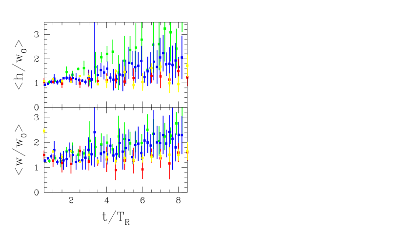
Figure 4: Average (points) and dispersion (error bars) over scaled height and width measurements made around ten randomly chosen particles as a function of time. The yellow and red points are for satellites of masses $10^{6}M_{\odot}$ and $10^{9}M_{\odot}$ respectively on the same orbit in a galaxy with spherical halo. The blue and green points are for a satellite of mass $10^{7}M_{\odot}$ on two different orbits in a galaxy with an oblate halo.

In this section we develop analytic expressions for the morphology of tidal streamers and compare them with the results of simulations of satellite galaxy destruction. In all these simulations, with the exception of those used for the blue and green points in Figure 4, the parent galaxy potential was fixed, with bulge, disk and halo components as described in the work of Johnston, Hernquist & Bolte (1996). In the other cases the halo potential was replaced by a flattened analog that generated the same rotation curve in the disk plane but had axis ratio $q=0.7$ in density. In all cases, the satellite galaxy was represented by particles initially distributed as a Plummer model, whose mutual interactions were calculated using a basis function expansion code (Hernquist & Ostriker (1992)). Table 1 summarizes the satellite and orbital properties used in the simulations and the papers in which they originally appeared.

Figure	$m_{\rm sat}$	$s$	$R_{\rm peri}$	$R_{\rm apo}$	$T_{\rm R}$	$T_{\rm sim}$	Paper
	$M_{\odot}$		kpc	kpc	Gyr	Gyr
1, 3	$10^{8}$	0.08	30	450	6.0	30.0	JCG01 (Model 4)
4, yellow	$10^{6}$	0.015	26	37	0.7	7.0	this paper
4, red	$10^{9}$	0.15	26	37	0.7	7.0	this paper
4, blue	$10^{7}$	0.029	45	135	2.2	19.7	this paper
4, green	$10^{7}$	0.034	25	60	1.2	19.7	this paper
5a	$10^{9}$	0.10	40	135	2.0	10	JHB96 (Model 1)
5b	$4\times 10^{7}$	0.04	41	175	2.7	10	JHB96 (Model 2)
5c	$2\times 10^{7}$	0.03	45	144	1.4	10	JHB96 (Model 3)
5d	$7\times 10^{6}$	0.07	20	140	0.9	10	JHB96 (Model 4)

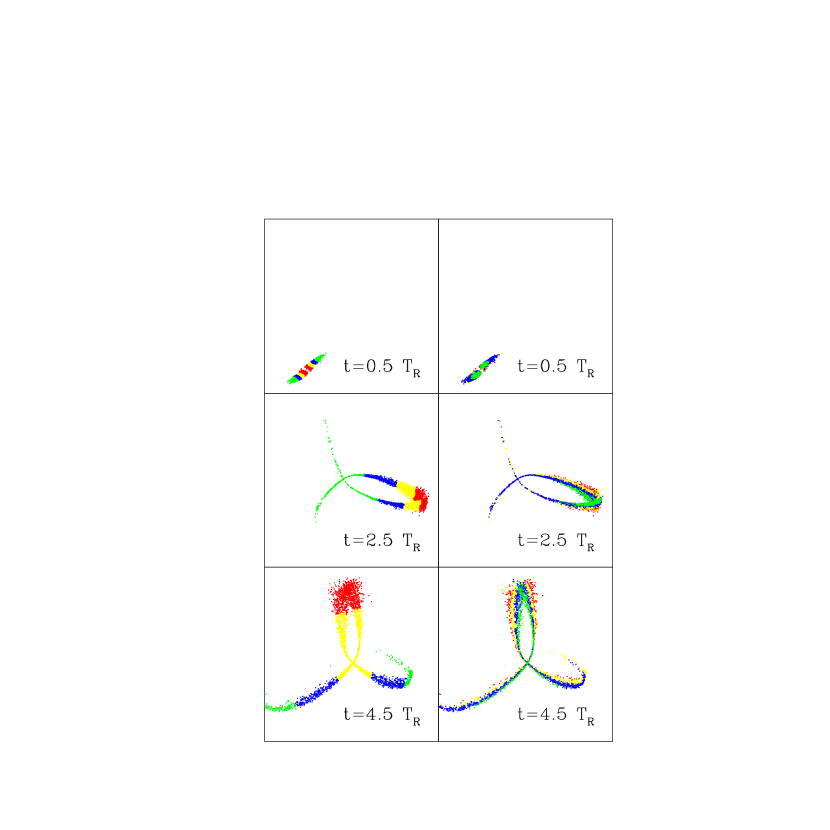
Figure 1: Positions in the orbital plane of particles at the end of a simulation of satellite disruption, color coded first by their orbital energies (left-hand panels) and then orbital angular momenta (right-hand panels) relative to the satellite’s orbit (the box size is 1000 kpc on a side). The red, yellow, blue, and green colors represent changes (scaled by $\epsilon$ and $j$) in the range $0.5-1.25,1.25-1.75,1.75-2.25$, and $2.25-3$, respectively.

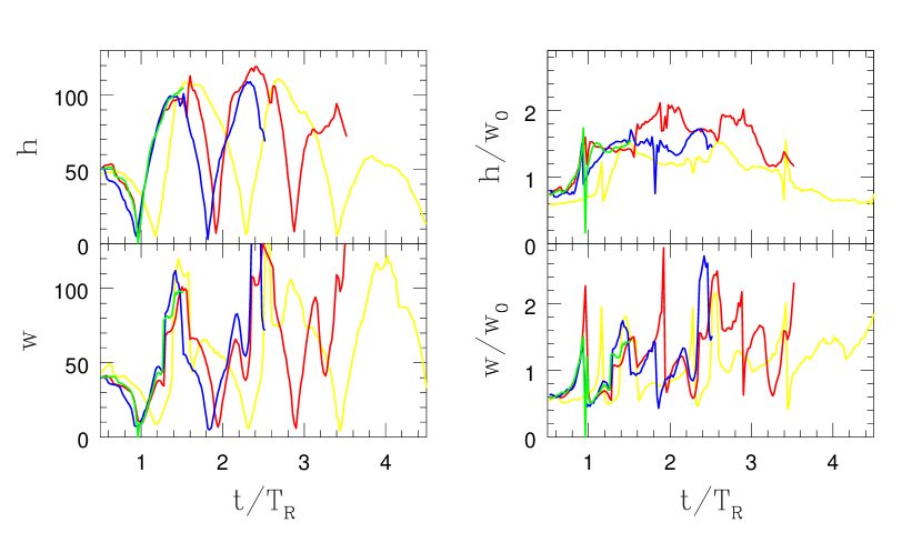
Figure 3: The left-hand panels present width and height measurements of debris as a function of time. The measurements were made around four particles lost on consecutive pericentric passages in a simulation. The right-hand panels scale these measurements by the expected initial height and width, $w_{0}$, given by equation (10).

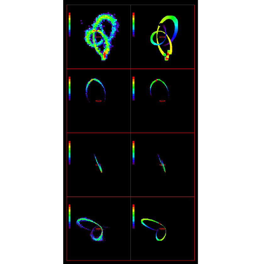
Figure 5: The left-hand panels show the surface brightness calculated from final positions of particles in four simulations of satellite destruction (see Table 1 for parameters) within a box $400\times 400$ kpc around the parent galaxy. In all cases the parent galaxy is lying edge on along the $X$-axis (indicated by the red ellipse) and the satellite orbits are viewed at random orientations. The color bar runs from $33-28$ mag/arcsec² in blocks of 0.5 mag in the R band, assuming a mass-to-light ratio $\Upsilon=10$. (Note that only the yellow and red portions of these streamers would be detectable with current techniques.) The right-hand panels show the corresponding predictions for the simulation results from semi-analytic methods in which the satellite mass, orbit, mass-loss rate and mass-to-light ratio are supplied as input.

Table 1: Parameters of satellites and orbits for the simulations used to test and illustrate our results in Figures 1–5 (with panels in Fig. 5 indicated by letters a–d from top to bottom). References in the last column: JCG01 – Johnston, Choi & Guhathakurta (2000); JHB96 – Johnston, Hernquist & Bolte (1996).

Tremaine (1993) and Johnston (1998) outline a simple physical picture for how debris from the destruction of a satellite orbiting in a near-spherical potential disperses along the satellite’s path. Here we extend their approach to describe the full geometry of tidal streamers. We expect our results to be valid when tidal streamers are dynamically young and still distinct in coordinate space — for example when following the dispersal of debris from small satellites that are disrupting in the near-spherical, outer halo of a galaxy where the timescale to mix fully along an orbit is longer than the age of the Universe. (We discuss what we mean by “small” and “outer halo” more fully in §2.3.3.) Helmi & White (1999) give a more rigorous treatment of debris dispersal applicable to a satellite orbiting in a static potential of any geometry and capable of following the full phase-space distribution of tidal debris as it becomes well-mixed — for example, to describe signatures of ancient accretion events in the inner halo.

In all equations below, the first equality holds for a tidal streamer in a general spherical potential $\Phi(R)$ and the second expression (following the arrow) is for the specific case of a logarithmic potential $\Phi=v_{\rm circ}^{2}{\rm log}(R)$, as might be appropriate for a galaxy with a flat rotation curve and circular velocity $v_{\rm circ}$. The equations can be applied in the regime in which the tidal scale $s\ll 1$, where

$$s\equiv\left({m\over M(R_{p})}\right)^{1/3}\,\longrightarrow\,\left({Gm\over v_{\rm circ}^{2}R_{p}}\right)^{1/3},$$ (1)

$m$ is the mass of the satellite, $M(R)=-(R^{2}/G)d\Phi/dR\longrightarrow v_{\rm circ}^{2}R/G$ is the mass of the parent enclosed within radius $R$, and $R_{p}$ is the pericenter of the satellite’s orbit (where mass loss predominantly occurs).

2.1 Dispersal Along the Satellite’s Path

The physical scale at which a satellite loses mass is given by its tidal radius

$$r_{\rm tide}=s\,R_{p}.$$ (2)

Thus, the specific orbital energies and angular momenta of the stars in the debris will be distributed about the satellite’s own orbital energy $E$ and angular momentum $J$ with a characteristic internal energy scale

$$\epsilon=r_{\rm tide}\left[{d\Phi\over dR}\right]_{R_{p}}\,\longrightarrow\,sv_{\rm circ}^{2}$$ (3)

and angular momentum scale

$$j=sJ~{}.$$ (4)

The time periods of orbits in a spherical potential depend more strongly on energy than on angular momentum (see e.g., Johnston 1998), so it is primarily the spread in energy $\epsilon$ within the debris that is responsible for the length of streamers seen in simulations of tidal disruption. After a time $t$, the debris will spread an angular distance of order

$$\Psi\sim 4\epsilon\left[{1\over T_{\Psi}}{\partial{T_{\Psi}}\over\partial{E}}\right]_{J=J_{\rm circ}}{2\pi t\over T_{\Psi}}\,\longrightarrow\,4s{2\pi t\over T_{\Psi}}$$ (5)

along the satellite’s orbit, where $T_{\Psi}$ is the azimuthal time period of a circular orbit of energy $E$. The factor of four reflects the fact that debris energies are predominantly spread in the range $-2\epsilon<\Delta E<2\epsilon$ around the satellite’s orbital energy (see Johnston 1998 and §2.2 below).

The discussion above indicates that once a set of stars becomes unbound from the satellite the constituents sort themselves in energy along a streamer. Hence, debris at a particular point along the streamer will have an average energy $\Delta E$ relative to the satellite’s orbital energy and will be offset correspondingly in radius from the satellite’s path by

$$\Delta R\sim\Delta E{dR\over d\Phi}\,\longrightarrow\,{\Delta E\over v_{\rm circ}^{2}}R~{}.$$ (6)

The concepts encapsulated in equations (3) and (5) are illustrated in the left-hand panels of Figure 1. These show the positions in the orbital plane of particles at three points during a satellite disruption simulation. In order to emphasize the evolution of a debris population with age, only those particles lost on the first pericentric passage of the satellite are plotted. The panels correspond to the first, third and fifth apocenter following this (hence when the debris is “age” 0.5, 2.5 and 4.5 $T_{R}$). The particles are color coded by orbital energies relative to the satellite’s orbit. The color coding clearly shows the particles sorting themselves in energy along the satellite’s orbit, with the extent of the debris along the orbit steadily increasing with time.

2.2 Dispersal Perpendicular to the Satellite’s Path

In contrast to the orbital time periods, the precession rate ($T_{R}/T_{\Psi}$) of the turning points of an orbit in a spherical potential depends primarily on the angular momentum of the orbit. Hence the spread in the angular momentum in the debris will cause the angular positions of the turning points of stars in the debris to spread out over time. This will lead to an increase in the streamer’s width in the orbital plane of order

$$w(R) = w_{0}+2jR\left({\partial{T_{R}/T_{\Psi}}\over\partial{J}}\right){2\pi t\over T_{\Psi}}=w_{0}+R\left[J{\partial{T_{R}/T_{\Psi}}\over\partial{J}}\right]s{4\pi t\over T_{\Psi}}$$ (7)

$$= w_{0}\left(1+\left[J{\partial{T_{R}/T_{\Psi}}\over\partial{J}}\right]{4\pi t\over T_{\Psi}}\right)$$ (8)

$$\,\longrightarrow\, w_{0}+R\left[J{\partial{T_{R}/T_{\Psi}}\over\partial{J}}\right]{\Psi\over 2},$$ (9)

where

$$w_{0}=w_{0}(R)=sR$$ (10)

is the width of the streamer at $R$ set by the initial spread in the turning points due to the tidal radius at pericenter. The factor of two prefacing the second term after the first equality reflects the fact that although the full range in angular momenta in the debris is of order $-2j<\Delta J<2j$ (analogous to the energy range described in the previous section), the spread at any point along the trail is of order $2j$ since negative (positive) angular momentum differences correspond to debris in leading (trailing) streamers.

Note that this description naturally explains the clear increase in the width of the streamers with $R$ in each of the panels of Figure 1: an angular offset between the turning points of debris particle orbits corresponds to a physical width that increases with $R$. The right-hand panels of this figure repeat the plots in the left-hand panels, but are now color coded according to the angular momenta of the particles relative to the satellite’s orbit. This coding illustrates how the particles sort themselves parallel to the orbit in angular momenta.

Since it is hard to visually assess the increase of the width of the streamers with time in Figure 1, the quantity in square brackets in equation (7) is plotted in Figure 2 as a function of angular momentum for a logarithmic potential, demonstrating that it is typically of order 0.05. This implies that the age $t$ of the streamer must be $t\sim(1/0.05)(T_{\Psi}/4\pi)\sim 1.5T_{\Psi}\sim 2.25T_{R}$ or larger (where the last equality comes from the range of precession rates in a logarithmic potential $0.6<T_{R}/T_{\Psi}<0.7$) before the streamer’s width starts increasing significantly beyond $w_{0}$, and that the streamer length $R\Psi$ will always be at least 10 times its width $w$.

Of course, in most instances the line of sight will not be perpendicular to the plane of a satellite’s orbit, so we must assess how debris will spread perpendicular to the satellite’s motion. In a spherical potential, the planar nature of the orbits guarantees that the debris will not spread perpendicular to the plane of the orbit beyond the height set at pericenter

$$h(R)\sim\left({r_{\rm tide}\over R_{p}}\right)R=s\,R\equiv w_{0}(R).$$ (11)

In non-spherical potentials, $h$ will increase with time due to the precession of the orbital plane in a manner analogous to the increase in width due to the precession of turning points in the orbital plane (Helmi & White (1999)).

We test the expectations outlined in this section more thoroughly in §2.3.1.

2.3 Tests of the Analytic Description

2.3.1 Evolution of Width and Height of Streamers

In this section we present plots of the width $w$ and height $h$ of streamers from a variety of simulations of satellite disruption, measured at several points along their length and at many different times. Each measurement was made at the position of a randomly-selected debris particle; the instantaneous plane of the orbit was defined at that point by the test particle’s position and motion. All particles lost during the same pericentric passage and located within $r_{\rm max}=0.25R/R_{\rm peri}$ of the test particle were labeled and ordered in distance from the orbital plane. The height $h$ was defined as the difference in the distances of the particles at the 10th and 90th percentile of the ordered set. To find a corresponding width, the above process was repeated for distances along axes defined in the orbital plane and centered on the test particle. Since the exact orientation of the stream was unknown, the results from 30 equally-spaced axis orientations were compared, and $w$ was taken to be the minimum of all these measurements.

The left-hand panels of Figure 3 illustrate the results of this analysis by plotting the evolution of $h$ and $w$ with time as measured around four test particles, each lost during different pericentric passages of the same simulation used in Figure 1. Time since the test particle was lost is expressed in units of the satellite’s radial orbital time period. The order-of-magnitude, periodic swings in the sizes of $h$ and $w$ are a reflection of the highly eccentric orbit of the satellite (which the debris closely tracks), with the smallest/largest values corresponding to the pericenters/apocenters of the particle’s orbit. Note that the increasing discrepancy between the time of these turning points is another signature of the debris drifting apart into streamers once it is lost.

The right-hand panels of Figure 3 present the same information as the left-hand panels, but are normalized at each point by the expected initial width, $w_{0}$, given in equation (10). This demonstrates that much of the behavior of the width and height of the debris is captured by this simple expression over the first few dynamical periods following disruption.

We tested this statement further using four more simulations with different satellite masses, orbits and parent galaxy potentials. Figure 4 displays the average of $h/w_{0}$ and $w/w_{0}$ measured around 10 test particles in debris populations lost on the first pericentric passage of each simulation (with the error bars indicating the dispersion) as a function of the time since that passage. The red and yellow points are for satellites on the same orbits, orbiting the same galaxy (with a spherical halo component), but with masses $10^{9}M_{\odot}$ and $10^{6}M_{\odot}$ respectively. These satellites have tidal scales $s$ that differed by a factor of 10, yet the points in the plot lie almost on top of each other. Note also that both $h$ and $w$ are increasing gradually with time because, even though the halo was perfectly spherical, the chosen orbit was fairly small (see Table 1) and the disk component of the parent galaxy caused some precession of the orbital plane. The blue and green points in the figure are for satellites of the same mass on two different orbits in a galaxy with an oblate halo. Here, the precession of the orbital plane is much more pronounced, which is reflected in faster growth of the width and height. We conclude that as long as the debris is no older than $t=4T_{R}$, equations (7) and (9) adequately describe the evolution of streamer height and width for a wide range of tidal scales, halo oblateness and orbital parameters.

2.3.2 Length and Surface Brightness Predictions

Johnston (1998) used the ideas encapsulated in equations (3) and (5) to understand the characteristics of debris dispersal seen in N-body simulations of the disruption of spherical stellar systems along a variety of orbits in a potential chosen to represent the Milky Way. She found that the debris in each simulation followed the same distribution in energies relative to the satellite’s orbit when scaled by the factor given in equation (3) over the range $-3\epsilon<\Delta E<3\epsilon$ (and predominantly in range $-2\epsilon<\Delta E<2\epsilon$ as noted above). Using this intrinsic distribution, she developed a semi-analytic method that could successfully reproduce the mass density along the tidal tails seen in any simulation, given the mass, orbit and mass loss rate of the satellite. This success confirms the predictive power of expressions in equations (3) and (5).

We tested the additional scalings derived above against the simulations of Johnston, Hernquist & Bolte (1996) by using the same methods to find the mass density and energy distribution along the streamers, and equations (10), (11) and (6) to predict the width and height of the streamers and their offset from the satellite’s orbit. The right-hand panels of Figure 5 show the surface density map produced using this semi-analytic method. The left-hand panels show the corresponding map produced from the actual final positions of particles in the simulations. The model successfully reproduces the position, geometry and surface density of the streamers produced by the simulations. In particular, note that at the point along the streamers where the surface brightness drops by roughly a magnitude from its maximum, the debris stars have $\Delta E\sim\pm 2\epsilon$, confirming the factor of four in equation (5) for our estimate of the streamer length.

2.3.3 Approximations Adopted

Figures 3 and 4 demonstrate that debris populations formed within the last few pericentric passages of a satellite in either spherical or mildly oblate potentials will have very similar width and heights that are not much greater than those set at disruption. Throughout the remainder of this work, we will assume that $w\sim h\sim w_{0}$ for $t<4T_{R}\sim 3T_{\Psi}$ is adequate for our purposes — from Figure 4 we estimate that this approximation is correct to within a factor of two either up or down (or within one magnitude in surface brightness) for all the times considered. Within this time we also expect debris streams to remain distinct in coordinate space for satellites with masses less than about 3% of the mass of their parent Galaxy that is enclosed within the pericenters of their orbits (or tidal factors less than $s_{\rm lim}=0.31$). We adopt this as a reasonable limit since we were able to predict (to within a factor of two) the width of the streamers in a simulation with $s=0.15$ for $>10T_{R}$ (red points in Figure 4). This translates to an upper limit $m_{\rm sat}^{lim}$ on the mass of the satellite that can be considered at a given radius. For example, for a satellite on an orbit with pericenter $R_{p}$ orbiting in a galaxy with circular velocity $v_{\rm circ}$, this limit is

$$m_{\rm sat}^{lim}=\left({s_{\rm lim}\over 0.31}\right)^{3}\left({v_{\rm circ}\over 200{\rm km/s}}\right)^{2}\left({R_{p}\over 10{\rm kpc}}\right)3\times 10^{9}M_{\odot}.$$ (12)

The above assumptions appear contrary to the findings of Helmi & White (1999) because they examined debris populations of ages $t>>4T_{R}$, with the aim of understanding the structure of the velocity distribution of debris stars. In fact, our estimates for the surface brightness of features in §3 (which are upper limits to the true surface brightness because of the above assumptions) suggest that even the best photometric observations of external galaxies today are not capable of detecting features much older than $t=4T_{R}$, either because they are too faint, or because of confusion by disk or halo light.

3 Observability

In external galaxies, debris trails generally will not be resolvable into individual stars. Instead, they will be recognized in deep wide-field photometry as elongated regions of enhanced surface brightness around a primary galaxy, perhaps still associated with a disintegrating satellite. In this section, we present a simple estimate for the surface brightness of a debris trail generated by a satellite of given properties orbiting in a known spherical potential. This approximate form is then used to assess the observability of trails as a function of their age, the mass of the satellite, and that of its parent body. At the end of this section, sources of confusing background are compared to the surface brightness of observable trails.

3.1 Surface Brightness of Debris Trails

Consider a satellite of mass $m$ and constant mass-to-light ratio $\Upsilon$ on a circular orbit at galactocentric radius $R$ around a galaxy with circular velocity $v_{\rm circ}$. If the satellite loses a fraction $f$ of its mass in the time $t$ that it takes the debris to spread through an angle $\Psi$ then, using equations (5) and (10), the debris is expected to have an apparent surface brightness (in mag/arcsec²) given by

$$\mu_{\nu}(t) = -2.5\,{\rm log}\left[{L_{\nu}\over L_{\odot,\nu}}\left({(10\,{\rm pc})^{2}\over wR\Psi}\right)\left(1\,{\rm arcsec}\over 1\,{\rm radian}\right)^{2}\right]+M_{\odot,\nu}$$ (13)

$$= -2.5\,{\rm log}\left[f\left({10M_{\odot}/L_{\odot,\nu}\over\Upsilon}\right){\left(1\,{\rm Gyr}\over t\right)}\right]$$

$$-{2.5\over 3}\,{\rm log}\left[{\left(v_{\rm circ}\over 200\,{\rm km/s}\right)}{\left(m\over 10^{8}M_{\odot}\right)}{\left(10\,{\rm kpc}\over R\right)}\right]+23.9+M_{\odot,\nu}~{},$$

where $M_{\odot,\nu}$ is the absolute magnitude of the Sun in the waveband of interest and $L_{\nu}=(f\,m/\Upsilon)L_{\odot,\nu}$ is the total luminosity of the debris trail. In this approximate representation, $w=h$ so that the surface brightness is independent of the inclination $i$ of the orbital plane to the sky plane. (This simplification is discussed in §2.2.)

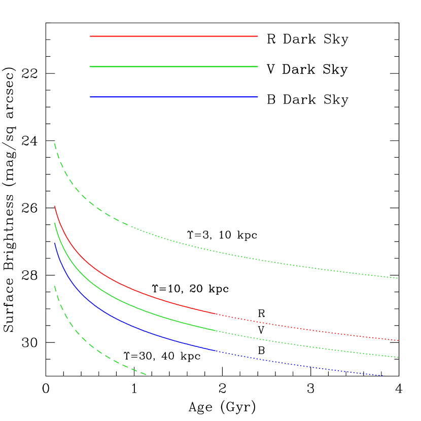
Figure 6: Expected surface brightness of tidal debris as a function of the age of the trail. Typical colors of Local Group dwarfs have been used. Solid lines indicate the surface brightness in $BVR$ expected for $10^{8}M_{\odot}$ satellites with mass-to-light $\Upsilon=10$ that have lost all their mass on circular 20 kpc orbits around primary galaxies with $v_{\rm circ}=200$ km/s. Also indicated for the $V$ band are two more extreme cases: a massive ($9\times 10^{8}M_{\odot}$) satellite with low $\Upsilon$ and tight orbit (upper dashed), and a small ($3\times 10^{7}M_{\odot}$) satellite with high $\Upsilon$ in a wide orbit (lower dashed.) The approximations used here are invalid for sufficiently old (dotted) streamers. For comparison, the surface brightness of a moonless night sky is also shown. Note that due to the typical colors of dwarfs and the dark sky, surface brightness limits for detection may be about $0.5-1.0$ mag fainter in $V$ than in $R$.

Figure 6 shows the temporal decay of surface brightness estimated from equation (13) resulting from the total destruction ($f=1$) of satellites similar to the dwarf galaxies in the Local Group. We have used a recent review of Local Group dwarfs (Mateo (1998)) as a guide to typical luminosities, colors and mass-to-light ratios, and have assumed that the primary has $v_{\rm circ}=200$ km/s, similar to that of the Milky Way. Shown as solid lines are the surface brightnesses in the $B$, $V$, and $R$ photometric bands for a $10^{8}M_{\odot}$ satellite with $\Upsilon=10$ pulled into a debris trail along its 20 kpc circular orbit. Such fiducial structural parameters are roughly compatible with the IC 1613 and Pegasus dwarf galaxies in the Local Group. The dotted extensions to these lines indicate when a streamer becomes too old dynamically ($t\geq 3T_{\Psi}\sim 3\times 2\pi R/v_{\rm circ}$) to allow the direct use of the analytical formulae in this paper, and these should be regarded as upper limits to the surface brightness.

The detection of such debris is not trivial, requiring surface brightness photometry reaching about 8 magnitudes below sky levels in these bands. At redder wavelengths, the sky brightness presents even more noise compared to the signal expected from dwarfs. The $B$-band luminosity and $B-V$ color of dwarfs varies widely depending on the presence of recent star formation. On balance, the $V$ or $R$ passbands may be the most reliable for the detection of tidal streamers in external galaxies. Satellites that are more luminous than our fiducial value ($L=10^{7}L_{\odot}$) either due to their larger mass, smaller $\Upsilon$, or both, and those satellites disrupted at smaller galactocentric radii ($R<20~{}$kpc) will generate brighter and thus more easily detectable trails. The opposite is true for less luminous satellites and those destroyed at larger radius. Two such extreme cases are shown for the $V$ passband as dashed lines in Figure 6. The brighter of these corresponds to the destruction of a $L=3\times 10^{8}L_{\odot}$, $\Upsilon=3$ dwarf similar to NGC 205 or M32 at 10 kpc from its parent galaxy. A satellite more like Phoenix or Carina, with $L=3\times 10^{6}L_{\odot}$ and $\Upsilon=30$ destroyed at 40 kpc would be too faint for detection with current techniques.

Strictly speaking, equation (13) is only valid for circular orbits; semi-analytic methods (Johnston (1998)) or N-body simulations can be used to predict variation in surface density along the length $\Psi$ for the case of eccentric orbits. In the following sections we use this approximation as a guide to the observability of dynamically young features around galaxies and in clusters. Debris generated more than about 4 Gyr ago would be expected to have surface densities too faint for detection with current capabilities; in any event, equation (13) is not suitable for debris older than a few radial periods since precessional effects would then cause it to fade faster than $t^{-1}$ (Helmi & White (1999)).

3.2 Astronomical Backgrounds and Target Selection

In the previous section, simple scaling arguments were used to show that if surface brightness levels $\sim$8 magnitudes below sky can be measured reliably, young tidal debris from satellites in near orbits around external galaxies can be detected (Fig. 6). With extreme care in observational technique and data reduction, such ultra-deep surface brightness photometry of galaxies is now being performed, generally for the purpose of studying normal, but faint, galactic components such as thick disks and stellar halos (Morrison, Boroson & Harding (1994); Fry et al. (1999); Matthews, Gallagher & van Driel (1999); Neeser et. al. (2000); Dalcanton & Bernstein (2000), and references therein), or intracluster light (Calcáneo-Roldán et al. (2000), and references therein). The very best of these have achieved detections (over large areas) at $R\approx$ 29 mag arcsec^-2. Only a handful of systems have been studied with sufficient resolution, depth and sky coverage to detect faint debris trails.

Streamers will be easier to interpret in terms of dwarf galaxy accretion if the surface brightness can be quantified and the parent’s morphology is largely undisturbed (suggesting that the dwarf’s effect on the parent — and hence on evolution of its own orbit — can be ignored). A natural sample to survey would be thin, edge-on disk galaxies in which the orientation is most favorable for detection of low-surface-brightness features and the existence of a well-behaved disk suggests that the parent is not significantly perturbed. Searches in dynamically active regions such as galaxy clusters may also yield interesting results, but must to be interpreted cautiously since material stripped from the primary galaxies and arcs associated with cluster-lensed background galaxies may be misinterpreted as debris trails from infalling material.

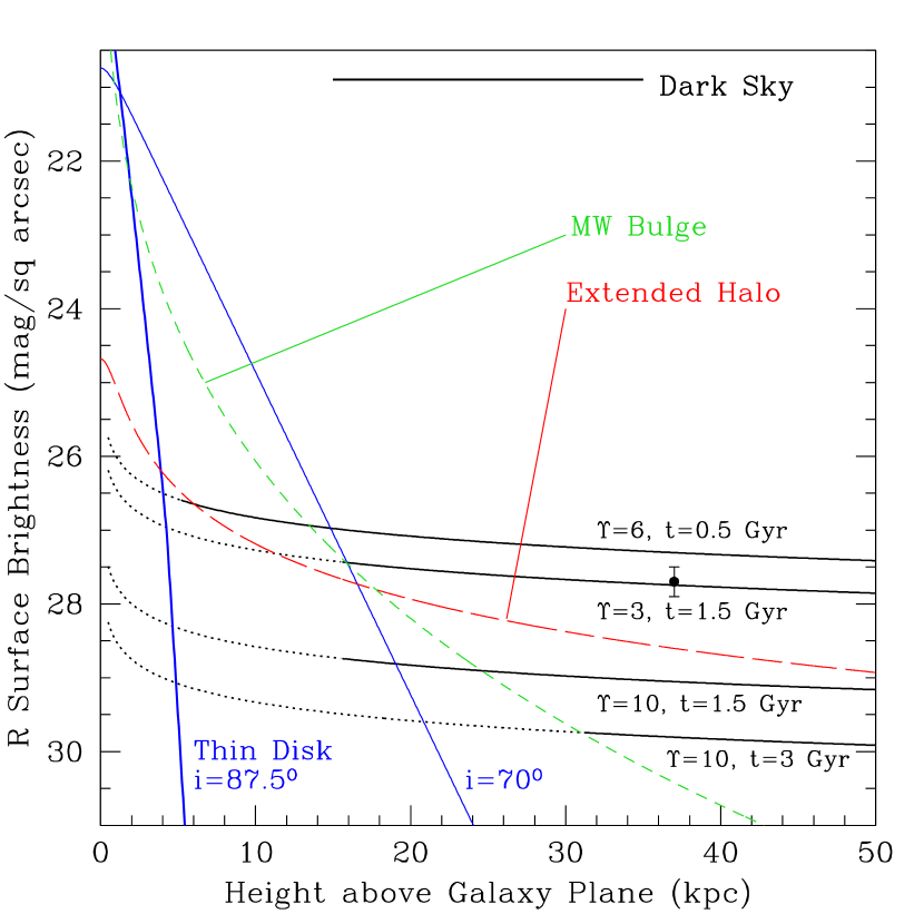
Figure 7: Expected R-band surface brightness of debris trails resulting from the destruction of a $10^{8}\,M_{\odot}$ satellite on a circular orbit around a thin spiral galaxy with $v_{\rm circ}=205\,$km/s, as a function of the orbital radius (height reached above the galaxy plane). A variety of streamer mass-to-light ratios $\Upsilon$ and ages $t$ are displayed (thin, black line). Regions for which the approximations used here (eq. 13) are likely to be invalid are indicated by dotted, black lines. For comparison, possible confusing sources of light from the galaxy itself are shown: a thin stellar disk inclined by angle $i$ with respect to the sky (blue, solid), a $R^{1/4}$ bulge such as that of the Milky Way (green, short-dash), and a fainter, more extended $r^{-2}$ halo (red, long-dash). The disk parameters ($i=87.5^{\rm o}$), faint extended halo, and $\Upsilon=3$, $t=1.5\,$Gyr streamer are appropriate to the observed and inferred parameters for thin edge-on spiral NGC 5907 at a distance of 14 Mpc. The data point is the measurement of Zheng et al. (1999). The surface brightness of a moonless R-band night sky is also shown.

Measurements of faint surface brightness enhancements near galaxies or in clusters are also challenging because in order detect extended features 8 mag fainter than sky at a $3\sigma$ level, all sources of statistical and systematic uncertainty that scale with sky brightness must be controlled to within 2 parts in 10⁵. In addition to the technical demands that this places on the required number of photons, the precision of detector calibration and the background (sky) level determination, the observer must also contend with astronomical sources of uncertainty due to confusing light from the galaxy itself and its environment. The behavior of the most common or troublesome astronomical sources of confusion is shown in Figure 7, together with the estimated surface brightness (from eq. 13) of streamers in circular orbits of a variety of radii around a typical disk galaxy. As in Figure 6, the dotted lines in Figure 7 trace features that are too old dynamically for interpretation using the analytical formulae in this paper; many of these features would also pass too near the disk plane of the primary to generate circular orbits.

Because the surface brightness of even young debris is so faint, galaxies that are viewed edge-on offer the best targets for streamer searches. We have chosen the edge-on Sc galaxy NGC 5907 to illustrate these effects in Figure 7, and will analyze a streamer around this galaxy in a later section. NGC 5907 is nearly bulgeless and is thin, with a scale length to scale height ratio of $h_{R}/h_{z}\approx 11$ (Morrison, Boroson & Harding (1994)). The surface brightness profile of its thin disk, which is inclined at about $i=87.5^{\rm o}$ to the sky plane, is shown as a function of height above the galaxy along its minor axis. The thin disk light of similar spirals will swamp that of reasonably bright debris streamers — even at heights of $\sim$20 kpc or more — if the galactic disk is inclined by $i\leq 70^{o}$.

Bulges, like that of Milky Way, are a source of unwanted of background light regardless of inclination angle, obscuring all but the very brightest debris within 20 kpc and a confusing factor out to 30–40 kpc for many streamers of reasonable age, $\Upsilon$, and total mass. Even much fainter spheroidal galactic components can complicate the detection of faint tidal debris if the light is sufficiently extended. Typical stellar halos of spirals have luminosity densities that decline with galactocentric radii like $r^{-3.5}$ or steeper (Saha (1985); Zinn (1985); Reitzel, Guhathakurta & Gould (1998)); these will provide a confusing background of light only at the smallest galactocentric radii. Some giant ellipticals and CD galaxies, on the other hand, have halo luminosities and globular cluster systems that fall less steeply, as $\sim r^{-2.3}$ (Harris (1986); Bridges, Hanes & Harris (1991); Harris, Pritchet & McClure (1995); Graham et al. (1996)). Such extended faint stellar halos may interfere with the detection of faint debris streamers. Indeed the surface brightness of the extended $r^{-2}$ halo reported in NGC 5907 inward of 10 kpc (Sackett et al. (1994); Lequeux et al. (1996); Rudy et al. (1997); James & Casali (1998)) is substantially brighter than the average surface brightness of its streamer seen at larger radii (Shang et al. (1998); Zheng et al. (1999)).

4 Applications

4.1 Interpreting the Remains of Disrupted Satellites

The intrinsic geometry of a streamer from a totally disrupted satellite can be used to estimate the mass $m$ and age $t$ of a young streamer, provided that the form of the galactic potential can be estimated. For example, rearrangement of equations (1), (5), and (10) for a logarithmic potential yields

$$m=s^{3}M(R_{p})=\left({w\over R}\right)^{3}M(R_{p})\sim 10^{11}\left({w\over R}\right)^{3}\left({R_{p}\over 10\,{\rm kpc}}\right)\left({v_{\rm circ}\over{\rm 200\,km/s}}\right)^{2}M_{\odot}~{},$$ (14)

and hence the mass-to-light ratio $\Upsilon$ of the satellite, and the time since its disruption

$$t\sim 0.01\,\Psi\left({R\over w}\right)\left({R_{\rm circ}\over 10\,{\rm kpc}}\right)\left({200\,{\rm km/s}\over v_{\rm circ}}\right){\rm Gyr}~{},$$ (15)

where $w$ is the width of the streamer at radius $R$, $\Psi$ is its angular length, and $R_{p}$ is the pericentric distance of the orbit. In the second equation we have replaced $T_{\Psi}$ by $2\pi R_{\rm circ}/v_{\rm circ}$ where $R_{\rm circ}$ is the radius of the circular orbit with the same energy as the true orbit. (Recall that the time periods of orbits depend primarily on their energy.) Of course, we cannot measure $R_{\rm circ}$ directly, but can approximate it as being halfway between the adopted apocenter and pericenter. Thus, for a logarithmic potential, the only information about the primary galaxy that one requires is an estimate of the circular rotation speed, which can be directly obtained from a measured rotation curve or the Tully-Fisher relation. The estimates of $m$ and $t$ depend only linearly on the cosmological distance to the galaxy.

More troublesome is the ambiguity introduced by the (generally) unknown inclination $i$ of the streamer to the sky plane at various positions along the orbit. In order to simplify the discussion, we assume that the streamer is co-planar, which is reasonable for the age of observable features. We define an orthogonal coordinate system with the $X$ and $Y$-axes in the plane of the sky and the $Z$-axis perpendicular to these along the line of sight. If the $Y$-axis lies along the intersection of the sky and orbital planes, then $R=R^{\rm obs}$ (where $R$ and $R^{\rm obs}$ are the true and observed distances from the center of the parent galaxy) along this axis, and $R=R^{\rm obs}/\cos i$ along the $X$-axis.

If the observed morphology of the streamer indicates that its orbit is nearly closed, we can assume that the orbit is nearly circular and $i$ can be estimated from the ratio of the observed semi-major $Y=a$ and semi-minor axes $X=b$ of the orbit, namely $\cos i=b/a$. In general, however, the orbit will not be closed and only a partial arc may be “illuminated” by detectable debris. In this case, the change of the width of the streamer along the arc can provide a useful diagnostic. Since we have assumed that $w=h$ at any point along the young streamer, projection has no effect on the observed width of the streamer, which does, however, increase with $R$ in any reasonable potential. The observed width $w$ of the streamer then becomes an indicator of relative galactocentric distance $R$ (with $R_{2}\approx R_{1}(w_{2}/w_{1})$ for any two points 1, 2 along the orbit in a logarithmic potential). For example, in the top panels of Figure 5 the orbit is face-on and the width of the streamers increase with projected distance from the galaxy, while in the third panels the orbit is nearly edge-on yielding a streamer with very different widths at similar projected radii.

As a final check, semi-analytic models or N-body simulations can be used to check the consistency of the measured surface brightness $\mu$ and width $w$ at several points along the feature for given model assumptions. An example of applying these simple ideas is presented in the following subsection.

4.1.1 Worked Example: NGC 5907

Shang et al. (1998) report the discovery of a partial “ring” of light around the edge-on disk galaxy NGC 5907. The arc is observed to be brightest and widest in the northeast half, where the average surface brightness is $28.0\pm 0.2$ mag arcsec^-2 in their intermediate band filter centered on 6660 Å, corresponding to about 27.7 mag arcsec^-2 in broadband R (Zheng et al. (1999)). The inferred broadband $R-I$ color is about $0.5\pm 0.3$, consistent with Local group dwarf satellites (Mateo (1998)). No gas has been detected in H$\alpha$ or HI emission lines associated with the arc of light. Shang et al. (1998) interpret the arc as debris from the destruction of a satellite on an elliptical orbit around the galaxy.

We adopt the satellite debris interpretation, but instead assume that the material is on a rosette rather than elliptical orbit, as is consistent with the assumption that NGC 5907 is embedded in a massive dark halo with circular velocity $v_{\rm circ}=205\,$km/s (deduced from VLA observations by Shang et al. (1998)). Furthermore, given the uncertainty introduced by the light from the galactic disk and obvious confusion from foreground stars along some portions assumed trajectory (the Shang et al. data were taken in 4 – 6″ seeing), we analyze only the clear northeast portion of the streamer, which subtends $\Psi\approx 2\pi/3$ radians of arc.

Assuming a distance to NGC 5907 of 14 Mpc (Zepf et al. (2000)) and the parameters given in Shang et al. (1998) and Zheng et al. (1999), the widest portion of the streamer has $w\sim 4.6\,$kpc and lies at a projected distance of $R^{\rm obs}=49\,$kpc from the center of the galaxy. The narrowest portion that can be observed cleanly lies just above the projected southeastern intersection of the streamer and galaxy at $R^{\rm obs}\approx 18\,$kpc, where the width is $w\sim 2.3\,$kpc. This latter position may or may not be the pericenter of the orbit, and is displaced by about $\pi/2$ from the widest portion of the streamer.

Since the width clearly increases with projected distance from the galaxy, it is reasonable to assume that the satellite’s orbit is not highly inclined with sky plane. The linear relationship between $w$ and $R$ in an isothermal potential suggests that the ratio of the true galactocentric distances of the widest and narrowest portions of the observed streamer is nearly equal to the ratio of their true widths. If the apparent major axis of the orbit lies near the sky plane, an inclination $i\sim 40^{\rm o}$ is implied. In this case, $R\approx R^{\rm obs}=49\,$kpc for the widest portion of the arc, whereas $R\approx R^{\rm obs}/\cos i=24\,$ kpc for the narrowest portion of the arc. Since tidal streamers lie inside or outside their satellite’s orbit depending on whether they are leading or trailing the satellite, we assume for the purposes of this illustration that $R_{p}=24$ kpc and $R_{\rm circ}=37~{}$kpc.

Inserting these values in equations (14) and (15), we estimate that the streamer comes from the destruction of a $m\approx 2\times 10^{8}M_{\odot}$ satellite $t\approx 0.8\,$Gyr ago. The mass-to-light ratio $\Upsilon$ of the progenitor can be estimated by noting that Shang et al. (1998) give a lower limit of $14.7\pm 3$ for the total apparent magnitude in the 6660 Å band, assuming that the streamer has its average detectable surface brightness throughout $2\pi$ radians. Converting to broadband R and considering only the $2\pi/3$ easily-detected arc, we obtain an estimate of $\leq 7\times 10^{7}\,L_{R,\odot}$ for the observed debris, and thus estimate that the debris trail has $\Upsilon_{R}\geq 3M_{\odot}/L_{R,\odot}$, or about $\Upsilon_{V}\geq 4M_{\odot}/L_{V,\odot}$. Given the uncertainties in the distance to NGC 5907 (Zepf et al. (2000)) and in the apparent magnitude of the debris, these mass-to-light ratios are uncertain by nearly a factor of two. These inferred satellite parameters are consistent with a progenitor similar to dwarf satellites such as NGC 185 or Pegasus in the Local Group, and the Fornax dSph (Mateo (1998)).

Because much of the angular length $\Psi$ may go undetected due to surface brightness constraints, the streamer’s age as estimated above is a lower limit on the time since satellite disruption. Indeed, the deep photometry of Shang et al. (1998) hint at a feature on the southwestern side of the galaxy, plausibly connected to the clearer arc on the other side, but making a sharp turn as the features cross the disk of NGC 5907 (in projection). If we interpret this feature as real and part of the debris trail, then $\Psi\geq 2\,\pi$ and the inferred age of the entire streamer increases to 2.4 Gyr. As a final check, the observed surface brightness of the ring (27.7 mag arcsec^-2 in broadband R, Shang et al. (1998); Zheng et al. (1999)) agrees with our analytical estimates for debris from a $2\times 10^{8}M_{\odot},\Upsilon=3$ satellite on a circular orbit at $R=37$ kpc with age in the range $0.8-2.4$ Gyrs (see Fig. 7).

We do not claim that these estimates are unique, particularly as they depend on the precise geometry of the streamer. Our estimates are, however, compatible with those of Reshetnikov and Sotnikova (2000), who conclude that the stellar arc around NGC 5907 has $\Upsilon_{B}\geq 3-7M_{\odot}/L_{B,\odot}$ and an age $t\leq 1.5\,$Gyr based on recent N-body simulations of the disruption of a dwarf companion moving in the polar plane of the NGC 5907 gravitational potential. Our independent semi-analytic simulations of this system, performed without knowledge of the Reshetnikov and Sotnikova work, confirm that the faint southwestern feature could plausibly be part of the same debris trail (see their Fig. 4).

4.2 Limits on the Mass Loss Rate from Observed Satellites

If we know that a satellite (with a dynamically-estimated mass) is at a projected distance from its parent (with measured $v_{\rm circ}$) but has no associated tidal tail to some limiting surface brightness $\mu_{\rm lim}$, we can place an upper limit on its fractional mass loss rate by re-arranging equation (13):

$${df\over dt}<\left({\Upsilon\over 10M_{\odot}/L_{\odot}}\right)\left[\left({200{\rm km/s}\over v_{\rm circ}}\right)\left({10^{8}M_{\odot}\over m_{\rm sat}}\right)\left({R_{p}\over 10{\rm kpc}}\right)\right]^{1/3}10^{{(M_{\odot,\nu}+23.9-\mu_{\nu,{\rm lim}})/2.5}}\,\,{\rm Gyr^{-1}}.$$ (16)

An example is given below.

4.2.1 Worked Example: Satellites of M31

name	$m_{\rm sat}$	$R^{\rm obs}$	$(M/L)_{V}$	$df/dt$
	$M_{\odot}$	kpc		Gyr-1
M32	$2.1\times 10^{9}$	5.4	5.6	$<$ 1.4
NGC 205	$7.4\times 10^{8}$	8.2	2.0	$<$ 0.85

Table 2: Properties of M31 satellites: the satellite mass, $m_{\rm sat}$; projected distance between the satellite and M31, $R^{\rm obs}$; mass-to-light ratio in the $V$ band; and upper limit on the fractional mass loss rate, $df/dt$. Observed quantities are from Mateo (1998).

Choi & Guhathakurta (2001) have recently completed a CCD mosaic of M31 which allows them to measure the outer isophotes of M32 and NGC 205 to a limiting surface brightness of $\mu_{B}=$27 mag/arcsec². Although their survey does reveal interesting features at low surface brightness levels close to each satellite, they are unable to trace these features beyond more than a couple of tidal radii. Adopting a value of $v_{\rm circ}=235\,$km/s (Braun (1991)) for M31’s dark halo we can calculate an upper limit to $df/dt$ for each satellite using their dynamical masses, observed $M/L$ and projected distances from M31 (see Table 2). This example is intended only as an illustration; at this limiting surface brightness level, the limits on $df/dt$ are very weak. In these particular cases, a stronger limit may be found by looking at the features close to each satellite (see Johnston, Choi & Guhathakurta (2000)).

4.3 Tidal Streamers and Galaxy Formation

Can cosmological models of galaxy formation be tested using a sensitive survey for debris trails?

N-body simulations naturally incorporate the physics of tidal disruption and debris dispersal. With additional assumptions about the relationship between the formation of stars and the dark halo in which they reside, the frequency of low surface brightness features observable around galaxies today could be predicted within a given cosmological model. This approach is limited by the resolution of the simulations to placing only lower limits on the number of trails we might expect to observe. First, as with identifying halos, there will be a mass limit below which a stream from a disrupted halo will not be resolved (presumably at higher mass than the satellite itself since the particles represent lower surface brightness features). Second, the finite resolution will cause random potential fluctuations that will scatter particles (i.e., numerical relaxation – see Weinberg (1993) for a general discussion) and tend to artificially reduce the surface brightness of debris streams. For example, Johnston, Spergel & Haydn (2001) found that a minimum of $10^{7}$ particles were needed in the parent Milky Way-like halo in order for a trail from a $10^{8}-10^{9}M_{\odot}$ satellite following an Sgr-like orbit to maintain its coherence over 4 Gyrs. This finding is clearly dependent on the mass and orbit of the satellite and the mass distribution in the parent galaxy, but nevertheless indicates the scale of the problem. It suggests that an appropriate N-body approach would be to simulate $\sim$100 such galaxies, each with $10^{7}$ particles within a cosmological context and then analyze them to assess the number of trails expected to be observed around a similar sample of real galaxies.

One way of testing whether such a computationally expensive study is warranted is to model satellite accretion history in a semi-analytic fashion that allows multiple realizations to be performed rather quickly, thus providing ample statistics and the ability to probe a large parameter space of input assumptions (e.g. Kauffmann, White & Guiderdoni (1993); Cole et al. (1994); Somerville & Primack (1999)). Current models of this kind use Monte-Carlo methods based on the extended Press-Schechter formalism (Kauffmann & White (1993); Lacey & Cole (1993); Somerville & Kolatt (1999)), and have proven successful at reproducing the merging histories of dark halos seen in N-body simulations (Lacey & Cole (1994); Somerville et al. (2000)). As with N-body simulations, associating galaxies and stars with dark halos must be done using some prescription. In addition, for application to satellite debris observations, some assumptions about the orbital distributions and the tidal disruption of the accreted objects must be made. The morphology and surface brightness of the streamers can then be predicted using methods presented here and in Johnston (1998). Unlike the N-body case, this approach, although less exact, suffers from no resolution limits.

4.3.1 Worked Example: Milky Way Satellite Debris in $\Lambda$CDM

As an illustration of this idea, we have used the model of Bullock, Kravtsov & Weinberg (2001) to provide the accretion histories of an ensemble of 100 halos, each with final $v_{\rm circ}=220$ km s^-1, which are assumed to host Milky Way-type galaxies. The model assumes a $\Lambda$CDM cosmology with $\Omega_{m}=0.3$, $\Omega_{\Lambda}=0.7$, $h=0.7$,and $\sigma_{8}=1.0$, and provides masses, approximate disruption times, and orbital evolution for each disrupted satellite. We estimate the mass-to-light ratios of the disrupted satellites by applying the same hypothesis used by Bullock, Kravtsov & Weinberg (2000) to match the observed abundance of Local Group satellites today: that low-mass satellites with virial temperatures below $\sim 10^{4}$K ($v_{circ}\lesssim 30$km s^-1) can only accrete gas before the universe was reionized at $z=z_{re}$. Under this assumption, the final baryonic mass of a satellite halo of mass $m$ will be $f_{m}m(\Omega_{b}/\Omega_{m})\simeq 0.14f_{m}m$. If $v_{circ}<30$ km s^-1, $f_{m}=f_{re}$ represents the fraction of the halo’s mass that was in place at $z=z_{re}$. (We assume $z_{re}=8$.) For halos with sufficiently deep potential wells ($v_{circ}>50$ km s^-1) the photoionizing background will not affect gas accretion, and $f_{m}=1.$ For intermediate masses, we assume that $f_{m}$ varies linearly between $f_{m}=f_{re}$ and $1$ as the halo size varies from $v_{circ}=30$ to $50$ km s^-1 (Thoul & Weinberg (1996)). Finally, if a fraction $\epsilon_{*}=0.5$ of this baryonic mass is converted to a stellar population with current mass-to-light ratio $M_{*}/L_{V}=2$, this implies $\Upsilon_{V}=30f_{m}^{-1}$. With $\Upsilon_{V}$ and the other disrupted satellite properties provided by the model, we then use equation (13) to estimate the surface brightness of features today.

The closed and open symbols in the top panel of Figure 8 indicate the final positions in the $\mu-R_{\rm circ}$ plane of all disruption events in our simulated ensemble that that satisfy our age criterion, $t<3T_{\Psi}$, and have occurred since each parent galaxy has accreted 90% of its mass. The latter requirement was imposed to ensure that additional orbit evolution of the debris is unlikely to be an important effect. Since the age of accretion events decreases with distance from the parent galaxy, one consequence of this requirement is that most of the trails have $R_{\rm circ}>50$ kpc. The trend of increasing $R_{\rm circ}$ with decreasing age also accounts for the fact that trails at large radii have higher average surface brightness than those at smaller radii.

Plotting against $R_{\rm circ}$ in Figure 8 does not directly illustrate the expected distribution of debris because most of the satellites were destroyed along eccentric orbits with $R_{p}<<R_{\rm circ}$. This is reflected in the distribution of the closed symbols which indicate the subset of these events that also satisfy our criterion, $s<0.31$. The total number of features brighter than a given surface brightness is shown in the bottom panel of Figure 8, indicating clearly that, within the chosen cosmology and star-formation prescription, we would expect to see many tens of features brighter than $\mu_{V}=30$ mag arcsec^-2 (about ten of which satisfy $s<0.31$ and hence are easiest to interpret) in such a survey of 100 parent galaxies. Moreover, these features tend to lie at large ($>50$ kpc) radii from their parent galaxy where they are less likely to be confused by background disk, bulge or halo light. (Fig. 7 shows that only very extended stellar halos are brighter than $\mu_{R}=29$ mag arcsec^-2 or $\mu_{V}=29.5$ mag arcsec^-2 at $R=50$ kpc.) We defer to a future paper a more complete discussion of the dependence of satellite debris characteristics on star formation prescription and cosmology. In the next section we discuss the feasibility of such an observational survey.

5 Observational Expectations for the Future

The apparent scarcity of observed debris streamers in external galaxies need not necessarily imply that they are not present, since the arguments we have presented indicate that most are probably at or below current detection levels. Special photographic emulsions may provide an excellent way of searching for such features over a wide field (Malin & Hadley (1997)), but calibration of the surface brightness levels needed for the best modeling will likely rely on charge coupled devices (Weil, Bland-Hawthorn & Malin (1997)). Since more photons are available for imaging than spectroscopy of individual lines, detection of low surface brightness features in external galaxies will always be easier than the measurement of their line-of-sight velocities.

For ease of detection, one would like:
           $[1]$ clear detection of diffuse light several magnitudes below sky
           $[2]$ simultaneous imaging of the complete streamer and the background sky
           $[3]$ minimal confusion from astronomical backgrounds
           $[4]$ control over systematic uncertainties, eg., flat-fielding and scattered light
The first goal requires a large number of photons, and the second a large detector. The third goal can be partially addressed with appropriate target selection (§3.2), while the last will require care in instrument design and observational strategy. In principle, the last goal is likely be the most difficult to achieve, but the first two are necessary, if not sufficient, conditions. We thus focus now on meeting the first and second goals with current and future instrumentation, namely the Advanced Wide Field Camera (ACS/WFC) on the 2.4m HST, the FORS imaging system on the 8m VLT, and proposed super-aperture telescopes, such as the 30 CELT or 100m OWL.

Using NGC 5907 as a guide, we consider the possibility of detecting a streamer with an observed length of 50 kpc and width of 5 kpc, to a depth that is one magnitude fainter than the average surface brightness R = 28 mag arcsec^-2 currently measured for the NGC 5907 arc. A rough upper limit to the physical size of the required field is 400 kpc, which allows 200 kpc on either side of the center of a galactic potential well for detection of satellite tails (see Figs. 6 and  8). The angular size of the required field will depend on the distance to the galaxy; a 400 kpc field corresponds to about 800″ at 100 Mpc. We now ask how long an integration time would be needed on various instruments in order to acquire the photons required for a $2\,\sigma$ detection of an area of the streamer equal to its typical width squared. Since a streamer might be expected to have a length at least 10 times its width (§2.2), the complete streamer would then lie $\sim$$6\,\sigma$ above the background noise.

Spaced-based observations such as those with the ACS/WFC have the advantage of low sky background, but also have smaller apertures relative to the most powerful ground-based imaging instrumentation. The $\sim$200″ field of the ACS/WFC is well-matched to primary galaxies at 400 Mpc, for which a total exposure of $\sim$1 hour is required to achieve the desired S/N with the standard configuration in typical conditions. The $\sim$400″ field size of the FORS imaging system on the VLT is suited to more nearby galaxies at distances of 200 Mpc, for which $\sim$12 minutes is required to reach the fiducial photon noise in typical, dark conditions on Paranal. A streamer of similar size, but $R$ = 30 mag arcsec^-2, would yield the required photon S/N in 1.5 hours with the VLT. The increased aperture afforded by planned telescopes such as CELT or OWL could reduce this time by factors of 3 to 10. Exposure times with the ACS could be halved if the search was resticted to streamers of similar angular (rather than physical) size as those probed by the VLT. In general, however, for the simple comparison made here, larger aperture wins over the reduced sky background.

We stress that the reliability of very faint detections will be dominated by systematics rather than photon noise, so that these estimates should be considered a strict lower limit to the total time required. Experience suggests that at surface brightnesses of $26<R<$ 28 mag arcsec^-2, systematic uncertainties are comparable to photon noise in their contribution to the error budget, so that exposure times 2 to 4 times longer than those estimated from photon statistics are required to realistically achieve the desired total S/N. At fainter levels, systematic uncertainties may completely dominate unless extreme care is taken in observational strategy and instrument design. Finally, note that imaging designed to reliably photometer debris streamers along their length will require considerably longer ($\times 10$) exposures than those aimed at detection only. Nevertheless, these estimates indicate that searches for young debris trails as faint as $R<$ 29 mag arcsec^-2 are feasible now around a sample of galaxies 200 Mpc distant from us. Planned super-aperture telescopes would allow the study of a fainter and older streamers around a larger sample of primaries.

6 Conclusions

We have developed and tested in this paper a simple semi-analytic formalism for following the surface brightness and morphology of debris during the first few orbits after a satellite is destroyed. Using the properties of Local Group satellites and extended light distributions around external galaxies we discussed to what extent the parent galaxy’s light should obscure such features. We then applied our models to three representative astronomical applications: (1) estimation of the mass-to-light ratio $\Upsilon$ and streamer age of the totally disrupted satellite responsible for NGC 5907’s debris arc, (2) derivation of the upper limit to the mass-loss rate $df/dt$ of partially-destroyed satellites such as would be expected for M32 or NGC 205, and (3) exploration of galaxy formation in a $\Lambda$CDM cosmology.

We find that the debris trail in NGC 5907 is well-modeled by disruption of a satellite with mass $m\approx 2\times 10^{8}M_{\odot}$ and mass-to-light ratio $\Upsilon_{R}=3$ originally on an orbit of approximate radius $R=37$ kpc disrupting $0.8-2.4$ Gyrs ago. We also find that the lack of very bright debris associated with the satellites of M31 indicates mass-loss rates $df/dt<1.5$ Gyr^-1. Finally, we find that a first examination of realizations of 100 galaxies in a standard $\Lambda$CDM cosmology, yields over forty features brighter than $\mu_{V}=$ 30 mag/arcsec². Such $V$ surface brightnesses are at the limit of current capabilities, but — if systematics can be controlled — may become routine with proposed telescopes such as OWL or CELT, allowing surveys for satellite debris in external galaxies to yield constraints on hierarchical models of galaxy formation.

Figure 2: The dependence of $J\,\partial(T_{R}/T_{\Psi})/\partial J$ (the quantity in square brackets in eq. (7)) on angular momentum for orbits in a scale-free logarithmic potential. In this case the quantity is independent of energy.

Figure 8: The top panel shows the position of debris in the $\mu_{V}-R_{\rm circ}$ plane in 100 semi-analytic realizations of galaxies. Only those points for disruption events that satisfy $t<3T_{\Psi}$, and that have occurred since the parent galaxy has accreted 90% of its mass are plotted. The filled points highlight those for which $s<0.31$. The bottom panel plots the cumulative number of trails brighter than a given limiting surface brightness.

References

- Braun (1991) Braun, R. 1991, ApJ, 372, 54
- Bridges, Hanes & Harris (1991) Bridges, T.J., Hanes, D.A., Harris, W.E., 1991, AJ, 101, 469
- Bullock, Kravtsov & Weinberg (2000) Bullock, J.S., Kravtsov, A.K., Weinberg, D.H., 2000, ApJ, 539, 517
- Bullock, Kravtsov & Weinberg (2001) Bullock, J.S., Kravtsov, A.K., Weinberg, D.H., 2001, ApJ, 548, 33
- Cole et al. (1994) Cole, S., Aragón-Salamanca, A., Frenk, C.S., Navarro, J.F., Zepf, S., 1994, MNRAS, 271, 781
- Calcáneo-Roldán et al. (2000) Calcáneo-Roldán, C., Moore, B., Bland-Hawthorn, J., Malin, D. and Sadler, E. M. 2000, MNRAS, 314, 324