Torque decay in the pulsar $(P,\dot{P})$ diagram

We investigate the evolution of pulsars in the $(P,\dot{P})$ diagram. We first present analytical formulae to follow the evolution of a pulsar using simple exponential models for magnetic field decay and alignment. We then compare these evolutionary tracks with detailed model calculations using ohmic decay of crustal neutron star magnetic fields. We find that, after an initial phase with a small braking index, $n$, pulsars evolve with enhanced torque decay ($n\gg 3$) for about 1 Myr. The long term evolution depends on the impurity parameter of the crust. If impurities are negligible in older isolated pulsars we expect their true age to be approximately equal to their observed characteristic age, $\tau=P/(2\dot{P})$. It is not possible from data to constrain model parameters of the neutron star crust.

1 Introduction

One of the key issues in pulsar physics is the question of torque decay. It is important to determine to what extent the braking torque decays in order to follow the dynamical evolution and calculate the true age of pulsars. The time dependent behaviour of the torque is closely linked to the important question of magnetic field decay and alignment of the magnetic and rotational axes of a neutron star.

In Fig. 1 we have plotted the rotational period, $P$, versus its derivative, $\dot{P}$, for 947 observed pulsars (F. Camilo, private communications). The pulsars evolve to the right in this diagram as they loose rotational energy. To date, only four pulsars (see Lyne et al. 1996 and references therein) have a measured value of $\ddot{P}$ (and the so-called braking index, $n=\Omega\ddot{\Omega}/\dot{\Omega}^{2}$, where $\Omega=2\pi/P$) which allows for a determination of the orientation of the evolutionary track in the $(P,\dot{P})$ diagram for the given pulsar at its present age. However, these four pulsars are all very young ($\tau\equiv P/2\dot{P}\simeq 2-15$ kyr) – otherwise $\ddot{P}$ is too difficult to measure. Thus we cannot learn much about long term torque decay from these observations.
Here we will first derive analytical evolutionary tracks by considering simple $\@vec{B}$-field decay and alignment. Both of these effects will give rise to enhanced torque decay and deviation from evolution along a straight line in the $(P,\dot{P})$ diagram. Thereafter we shall present evolutionary tracks calculated from ohmic decay of crustal neutron star magnetic fields. Such calculations of the neutron star crust were introduced by Sang & Chanmugam (1987) and Urpin & Muslimov (1992) who also included cooling models.

The millisecond pulsars ($P\la$ 0.1 sec and $\dot{P}\la 10^{-17}$) are seen to form a separate population in the $(P,\dot{P})$ diagram shown in Fig. 1 – presumably as a result of their binary origin (Alpar et al. 1982; van den Heuvel 1984). In this paper we shall only concentrate on the evolution of isolated pulsars. For calculations of accretion-induced magnetic field decay of a binary neutron star (the millisecond pulsar progenitor) see e.g. Geppert & Urpin (1994), Urpin, Geppert & Konenkov (1997), Konar & Bhattacharya (1997; 1999).

We outline the dynamics of a rotating neutron star in Sect. 2. In Sect. 3 we discuss a simple combined model with exponential magnetic field decay and alignment. In this section we also discuss the observed data and evidence for enhanced torque decay, as well as the role of the inclination angle with respect to the braking torque. A detailed model of the crustal physics of a cooling neutron star is used in Sect. 4 to calculate more realistic evolutionary tracks in the ($P,\dot{P}$) diagram. Finally, the conclusions are briefly summarized in Sect. 5.

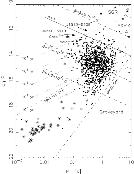
Figure 1: Distribution of 947 observed pulsars in the $(P,\dot{P})$ diagram. Binary pulsars are marked with a circle. The four pulsars with measured braking index evolve along the direction of the arrows. The solid line is an evolutionary track with $n=3$. The dotted and dashed lines represent constant characteristic age and constant magnetic field, respectively. When radio pulsars cross the “death line” their emission is terminated as a result of the low electrostatic potential drop across their polar cap. In the top right corner is plotted observations of soft $\gamma$-ray repeaters (SGR) and anomalous X-ray pulsars (AXP).

2 The rotating neutron star

In the following section we shall concentrate on the “slow” (non-recycled) pulsars whose evolution is not “polluted” by interaction with a companion star.
Consider a neutron star with moment of inertia, $I$ and angular frequency, $\Omega$. Its rotational angular momentum and spin period is given by:

$$L=I\Omega\qquad P=2\pi/\Omega$$ (1)

The rotational energy and its loss rate are given by:

$$E_{\rm rot}=\frac{1}{2}I\Omega^{2}\qquad\dot{E}_{\rm rot}=I\Omega\dot{\Omega}$$ (2)

The braking torque acting on the neutron star is thus:

$$N\equiv\frac{dL}{dt}=I\dot{\Omega}=\dot{E}_{\rm rot}/\Omega$$ (3)

(if we assume that $I$ is constant in time).
For an isolated neutron star $\dot{E}_{\rm rot}<0$, and hence $N<0$. The change in magnitude of the torque as a function of time is given by:

$$\frac{d|N|}{dt}=-I\ddot{\Omega}$$ (4)

The term “torque decay” thus refers to a decrease in the magnitude of the torque. Hence, the needed condition is:

$$\frac{d|N|}{dt}<0\quad\Longleftrightarrow\quad n>0$$ (5)

where we have introduced the braking index, $n$ defined as:

$$n\equiv\frac{\Omega\ddot{\Omega}}{\dot{\Omega}^{2}}=2-\frac{P\ddot{P}}{\dot{P}^{2}}$$ (6)

By introducing the characteristic age, $\tau\equiv P/(2\dot{P})$ we can get an idea of how $|N|$ decreases with the age of a pulsar:

$$N=I\dot{\Omega}=-\pi I\frac{1}{\tau P}\quad\rm{or}\quad|N|\propto\frac{1}{\tau P}$$ (7)

2.1 Torque decay and braking index in the magnetic-dipole model

In the magnetic-dipole model (Pacini 1967, 1968; Ostriker & Gunn 1969) the spin-down energy is carried away by magnetic dipole radiation:

$$\dot{E}_{\rm rot}=I\Omega\dot{\Omega}=-\frac{2}{3c^{3}}|\ddot{\@vec{m}}|^{2}=-\frac{2B^{2}R^{6}\Omega^{4}\sin^{2}\!\alpha}{3c^{3}}$$ (8)

where $R$ is the radius of the neutron star, $B$ is the strength of the dipole component of the magnetic field at its equatorial surface, $\@vec{m}$ is the magnetic dipole moment and $\alpha$ is the inclination of the magnetic axis with respect to the rotation axis. Hence, in this model the braking torque (i.e. the radiation-reaction torque) transmitted to the neutron star by the magnetic field is proportional to $B^{2}\,\sin^{2}\!\alpha$. From the above equation one obtains:

$$P\dot{P}=\left(\frac{8\pi^{2}R^{6}}{3c^{3}I}\right)B^{2}\;\sin^{2}\!\alpha=\frac{1}{k^{2}}\,B^{2}\sin^{2}\!\alpha$$ (9)

where we have assumed $k\equiv\sqrt{\frac{3}{8}c^{3}I}/\pi R^{3}$ is a constant.

3 Evolution with $\@vec{B}$-field decay and alignment

Soon after the discovery of pulsars Ostriker & Gunn (1969) suggested that the magnetic field of a neutron star should decay exponentially on a time-scale $\tau_{D}\sim 4$ Myr, because of ohmic dissipation of the supporting currents. The same authors also presented observational evidence in favour of field decay (Gunn & Ostriker 1970). However, it was soon argued by others that the ohmic decay cannot be important since the interior of a neutron star is likely to be superconducting (Baym, Pethick & Pines 1969). Ever since the early days of pulsar astronomy this important question of magnetic field decay has continued to be rather controversial, see e.g. Bhattacharya & Srinivasan (1995) for a review on this matter.
Let us for a moment assume an exponential field decay:

$$B(t)=B_{0}\,e^{-t/\tau_{D}}$$ (10)

where $\tau_{D}$ is the time-scale of decay and $B_{0}$ is the strength of the surface dipole magnetic field at time $t_{0}=0$.

Over the years, many authors have argued for or against observational evidence that the magnetic axis aligns with the rotation axis: Proszynski (1979), Candy & Blair (1983,1986), Lyne & Manchester (1988), McKinnon (1993), Gould (1994) and Gil & Han (1996). Beskin et al. (1988) even argue in favour of counter-alignment based on their magnetospheric theory. Recently Pandey & Prasad (1996) and Tauris & Manchester (1998) argue in favour of alignment. It is therefore important to investigate the evolution of the braking torque since this could be significantly influenced by the alignment process. The idea that the magnetic axis aligns with the rotation axis was first analyzed analytically by Jones (1976). He suggested a simple exponential decay of the inclination angle, $\alpha$ of the form:

$$\sin\alpha(t)=\sin\alpha_{0}\,e^{-t/\tau_{A}}$$ (11)

where $\tau_{A}$ is the alignment constant and $\alpha_{0}$ is the initial inclination angle at the time $t_{0}=0$.

Inserting the two above expressions into Eq. (9) and integrating yields the period evolution of a pulsar in the general case including both exponential magnetic field decay and alignment:

$$P^{2}(t)=\Pi_{0}\,\tilde{\tau}_{D}\,(1-e^{-2t/\tilde{\tau}_{D}})+\,P_{0}^{2}$$ (12)

where $\Pi_{0}\equiv P_{0}\dot{P}_{0}=(B_{0}\,\sin\alpha_{0}/k)^{2}$. We have introduced an effective reduced time scale, $\tilde{\tau}_{D}\equiv\frac{\tau_{D}\tau_{A}}{\tau_{D}+\tau_{A}}$ due to the symmetry of Eqs (10) and (11).
Using Eqs (3), (9), (12) and $\dot{\Omega}=-2\pi\dot{P}/P^{2}$ gives the time dependence of the braking torque:

$$N(t)=\frac{-2\pi I\,\Pi_{0}\;e^{-2t/\tilde{\tau}_{D}}}{\left[\Pi_{0}\,\tilde{\tau}_{D}\,(1-e^{-2t/\tilde{\tau}_{D}})+P_{0}^{2}\right]^{3/2}}$$ (13)

A simple differentiation of Eq. (8) yields:

$$\ddot{\Omega}(t) = -\frac{4R^{6}B(t)\dot{B}(t)\sin^{2}\!\alpha(t)}{3c^{3}I}\;\Omega^{3}(t)$$ (14)

$$-\frac{4R^{6}B^{2}(t)\sin\alpha(t)\cos\alpha(t)\,\dot{\alpha}(t)}{3c^{3}I}\;\Omega^{3}(t)$$

$$-\frac{2R^{6}B^{2}(t)\sin^{2}\!\alpha(t)}{c^{3}I}\;\Omega^{2}(t)\,\dot{\Omega}(t)$$

and hence we have an expression for the braking index:

$$n(t)=3 - \frac{3c^{3}I\dot{B}(t)}{R^{6}B^{3}(t)\sin^{2}\!\alpha(t)\,\Omega^{2}(t)}$$ (15)

$$- \frac{3c^{3}I\cot\alpha(t)\,\dot{\alpha}(t)}{R^{6}B^{2}(t)\sin^{2}\!\alpha(t)\,\Omega^{2}(t)}$$

or simply:

$$n(t)=3-F(t)\,\frac{\dot{S}}{S}$$ (16)

where

$$F(t)\equiv[3c^{3}I]/[R^{6}B^{2}(t)\sin^{2}\!\alpha(t)\,\Omega^{2}(t)]$$ (17)

and

$$S=\left\{\begin{array}[]{llll}B(t)\,\sin\alpha(t)&\mbox{\hskip 2.84544ptfor B-decay and alignment}\\ B(t)&\mbox{\hskip 2.84544ptfor B-decay only}\\ \sin\alpha(t)&\mbox{\hskip 2.84544ptfor alignment only}\\ B_{0}\,\sin\alpha_{0}&\mbox{\hskip 2.84544ptfor const. B and no alignment}\\ \end{array}\right.$$ (18)

From the above equations we immediately obtain the allowed values of $n(t)$, depending on the effect acting on it (cf. Table 9.1 of Manchester & Taylor 1977):

$$n(t)\left\{\begin{array}[]{llll}>3&\mbox{\hskip 8.5359ptfor}&\mbox{\hskip 2.84544pt$\dot{B}<0\;\;{\rm and/or}$}&\mbox{\hskip 2.84544pt$\dot{\alpha}<0$}\\ <3&\mbox{\hskip 8.5359ptfor}&\mbox{\hskip 2.84544pt$\dot{\alpha}>0\,\;\;{\rm and}$}&\mbox{\hskip 2.84544pt$\dot{B}\not<0$}\\ =3&\mbox{\hskip 8.5359ptfor}&\mbox{\hskip 2.84544pt$\dot{B}=0\;\;{\rm and}$}&\mbox{\hskip 2.84544pt$\dot{\alpha}=0$}\\ \end{array}\right.$$ (19)

where $\dot{\alpha}>0$ corresponds to the case of counter-alignment.

3.1 Constant magnetic field and no alignment

A Taylor expansion of Eqs (12), (13) and (15) for $\tau_{D}\rightarrow\infty$ or/and $\tau_{A}\rightarrow\infty$ yields the period, torque and braking index in case of a constant magnetic field, no alignment or both. For example, if we assume no field decay and no alignment ($\tau_{D}\rightarrow\infty$ and $\tau_{A}\rightarrow\infty$) we obtain:

$$P^{2}(t)=2\,\Pi_{0}\;t+\,P_{0}^{2}$$ (20)

$$N(t)=\frac{-2\pi I\,\Pi_{0}}{(2\,\Pi_{0}\;t+P_{0}^{2})^{3/2}}$$ (21)

$$n=3$$ (22)

3.2 Results

In the top panels of Fig. 2 we have plotted evolutionary tracks in the $(P,\dot{P})$ diagram for various values of $\tilde{\tau}_{D}$ and $\Pi_{0}$. In the left panel we have plotted evolutionary tracks calculated without enhanced torque decay. The right panel shows evolutionary tracks including enhanced torque decay. For each initial starting point three curves are plotted corresponding to an increasing time scale, $\tilde{\tau}_{D}$ (from left to right). We have assumed $k=3.2\times 10^{19}$ g${}^{\frac{1}{2}}$ cm${}^{-\frac{1}{2}}$ s${}^{-\frac{3}{2}}$. The small dots represent data of observed pulsars. It is seen that many evolutionary tracks fitting the data can be obtained from different choices of $\Pi_{0}$ and $\tilde{\tau}_{D}$. The thin lines in the top left panel are isochrones of 0, 1, 5, 10, 50, 100, 500 kyr, 1, 5, 10, 50 and 80 Myr, respectively.

To illustrate the difference between an evolution without ($\tilde{\tau}_{D}=\infty$) and with ($\tilde{\tau}_{D}$ = 10 Myr) enhanced torque decay (due to magnetic field decay, a multipole or alignment) in Fig. 2 we have also plotted $P$, $n$, $\tau$ and $N$, calculated from the equations derived earlier as a function of the true age, $t$.

Figure 2: The top two panels show various evolutionary tracks in the $(P,\dot{P})$ diagram. The assumed time-scales for enhanced torque decay are written in each panel. The bottom four panels show $P,n,\tau$ and $N$ as a function of true age, $t$ – see text.

Figure 3: Dependence of the pulsar slow-down on the braking index, $n$. The spin period, $P$ is plotted as a function of true age, $t$ for $n=2$, $n=3$ and $n>3$ ($\tilde{\tau}_{D}=10$ Myr). For $n=3$ the slope of the curve is given by: $\dot{P}=P/(2t)$ and hence $t=\tau$ (where $P>\!\!>P_{0}=10.0$ ms). In Table 1 is given the relation between true age, $t$ and characteristic age, $\tau$ for the different values of $n$.

Table 1: Values of true age ($t$), characteristic age ($\tau$), spin period ($P$) and braking index $n(t)$ for three different models of evolution (birth parameters: $P_{0}=10$ ms and $\log\dot{P}_{0}=-12.5$).

	$n=2$		$n=3$		$n>3\quad\tilde{\tau}_{D}=10$ Myr
$t$	$\tau$	$P$	$\tau$	$P$	$\tau$	$P$	n(t)
Myr	Myr	s	Myr	s	Myr	s
0.01	0.01	0.10	0.01	0.05	0.01	0.05	3.00
0.03	0.02	0.31	0.03	0.08	0.03	0.08	3.01
0.10	0.05	0.99	0.10	0.14	0.10	0.14	3.04
0.32	0.16	3.14	0.32	0.25	0.33	0.25	3.13
1.00	0.49	9.94	1.00	0.44	1.10	0.42	3.44
3.16	1.57	31.4	3.16	0.79	4.39	0.68	4.77
10.0	4.98	99.4	10.0	1.41	31.8	0.93	15.8
31.6	15.7	314	31.6	2.51	2774	1.00	1118
100	49.8	994	100	4.46	$>10^{9}$	1.00	$>10^{8}$

The evolution with enhanced torque decay (solid line, $n>3$) is clearly seen to result in a strong decay of the braking torque for $t>\tilde{\tau}_{D}$ and hence a strong decrease of $\dot{P}$ ($\dot{P}\rightarrow 0$). Therefore a constant value of $P$ is approached as the radio emission process becomes inactive after 10–50 Myr (while the pulsar crosses the so-called death line). The strong decrease in $\dot{P}$ has an important influence on the braking index which accordingly increases sharply when $t\rightarrow\tilde{\tau}_{D}$ (see Eq. 6, $\ddot{P}<0$). This is shown in the central right panel.

If pulsars evolve without magnetic field decay or alignment (dashed line, $n=3$) they will attain much larger ages before they cross the death line. For these pulsars the true age, $t$ will always be equal to the observed characteristic age, $\tau=P/2\dot{P}$ ($P\gg P_{0}$) – whereas if enhanced torque decay is important ($n>3$) the true age of pulsars will be smaller than $\tau$ (in this case by more than an order of magnitude for $\tau>20$ Myr).
In Fig. 3 we have demonstrated this effect graphically. The tangent to the $n=3$ curve at a given age, $t$ will always intersect the x-axis ($P=0$) at $t_{x}=-t$. Thus the slope of this tangent is $\dot{P}(t)=P(t)/2t$, or equivalently $t=P(t)/2\dot{P}(t)$ which is equal by definition to the characteristic age, $\tau$. The tangent to the $n>3$ curve is seen to be less steep and therefore $\dot{P}(t)<P(t)/2t$, or $t<\tau$. Finally, in the case of relaxed torque decay ($0<n<3$, e.g. radial deformation of $\@vec{B}$ or a decreasing moment of inertia in young pulsars) we have $t>\tau$.

For population statistics and evolution of pulsars it is therefore essential to know whether or not enhanced torque decay occurs in order to determine the true ages of the observed pulsars.
It should be noted, that strictly speaking the braking index, $n$ is defined from the power-law: $\dot{\Omega}\propto-\Omega^{n}$. However, in general $n$ is a function of time: $\dot{\Omega}=\Lambda(t)\,\Omega^{n(t)}$ and since there is no analytical solution to this power-law equation, we have retained the definition of $n$ as given in Eq. (6).

3.3 Observational evidence on torque decay ?

Many attempts have been made to find observational evidence for magnetic field decay. The key problem (as outlined above) is that we do not know the true age of the pulsars observed. Furthermore, many parameters connected to pulsars (e.g. $\tau$ and $B$) are given as functions of the two fundamental observed parameters: $P$ and $\dot{P}$. There are many different ways to illustrate the evolution of pulsars. Here, we introduce another variant of the $(P,\dot{P})$ diagram and plot the rotational energy of a pulsar as a function of its characteristic age. This is shown in Fig. 4. The dashed lines represent evolution with $n=3$ (constant $B$-field and magnetic inclination angle) and the solid lines are calculated with enhanced torque decay ($n>3,\tilde{\tau}_{D}=10$ Myr). In each case we considered two different sets of initial birth parameters for the pulsar: ($P_{0}=10.0$ ms, $\log\dot{P}=-13.5\Rightarrow B_{0}=5.69\times 10^{11}$ G) and ($P_{0}=31.6$ ms, $\log\dot{P}=-12.0\Rightarrow B_{0}=5.69\times 10^{12}$ G). If pulsars evolve without enhanced torque decay they should move along the dashed lines. If enhanced torque decay is important their evolution should bend off along the solid lines.

We have shaded two regions in the diagram (A and B) where there is a deficit of pulsars. If pulsars evolve with $n=3$, the region A should feed pulsars into the relatively dense populated area near the arrowhead. Similarly, region B should be the endpoint of pulsars coming from the populated area along its arrow base. So why are there so few pulsars in region A and B ? A simple reason for the few pulsars in region A could be due to the logarithmic scale for the characteristic age. Hence, the pulsars accumulate with time near the arrowhead before crossing the death line. However, if this is the correct explanation it seems strange why there should not be a similar effect below this region, e.g. between and parallel to the dashed lines. Furthermore, the deficit of pulsars in region B is even more strange in this respect (since pulsars are then supposed to be accumulated in this region), unless the naively drawn death line in reality bends into this region. In both cases we notice that a natural explanation, for the deficit of pulsars in the shaded regions, is the effect of enhanced torque decay and subsequent bending of the evolutionary tracks. We will let the reader draw his own conclusion.

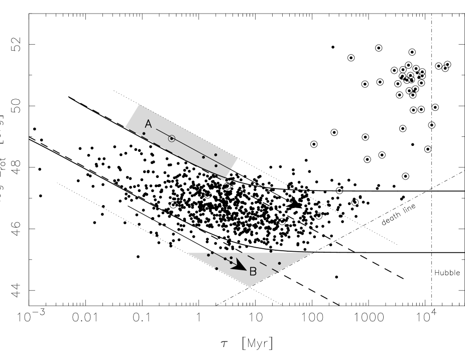
Figure 4: The rotational energy of observed pulsars plotted as a function of their characteristic age. The solid and dashed lines are evolutionary tracks with and without enhanced torque decay, respectively. We assumed a pulsar moment of inertia, $I=10^{45}$ g cm². The millisecond pulsar population is seen in the upper right corner. See text for discussion.

Figure 5: A plot of $\dot{P}/P^{2}$ vs. the observed inclination angle, $\alpha_{\rm obs}$. The top panel contains 316 pulsars obtained from Gould (1994) and the bottom panel shows 149 pulsars from Rankin (1993) – see Tauris & Manchester (1998) for details. The braking torque, $N\propto\dot{P}/P^{2}$ is seen to be a slightly increasing function of $\alpha_{\rm obs}$. Standard error bars of the binned mean values are plotted.

3.3.1 Torque decay and the magnetic inclination angle

In the Goldreich-Julian (1969) model of a non-vacuum magnetosphere of a pulsar, the slow-down of rotation is caused by outflow of plasma:

$$\dot{E}_{\rm rot}=-\left(\frac{B_{\rm L}}{8\pi}\right)^{2}4\pi R_{\rm L}^{2}\,c$$ (23)

where $R_{\rm L}=c/\Omega$ is the radius of the light cylinder and $B_{\rm L}$ is the magnetic field strength at this location – for a dipole field: $B_{\rm L}\propto 1/r^{3}$ or $B_{\rm L}=B\,(R/R_{\rm L})^{3}$. This expression for $\dot{E}_{\rm rot}$ is of the same magnitude as in Eq. (8), but here the braking torque ($N=\dot{E}_{\rm rot}/\Omega$) is independent of $\alpha$. The dynamics of a rotating neutron star in this case is then similar to that of the magnetic-dipole model for a constant inclination angle. In Fig. 5 we have plotted the braking torque, $N\propto\dot{P}/P^{2}$ vs. the observed inclination angle, $\alpha_{\rm obs}$ for a large number of pulsars. The derived, observed magnetic inclination angles were taken from the work by Tauris & Manchester (1998) and references therein. Though we cannot rule out the possibility that $N$ is independent of $\alpha$ (a $\chi^{2}$-test yields a $\sim 15$ % probability for constancy) we notice that $N$ seems to be a slightly increasing function of $\alpha$ (although the scatter is large). However, we must also bear in mind that $\alpha$ itself is only a marginally decreasing function of characteristic age (see Tauris & Manchester 1998). Hence, based on observations the effect of $\alpha$ on $N$ is probably not a major concern.

We have now demonstrated how simple analytic models can account for the distribution of observed pulsars in the $(P,\dot{P})$ diagram, although the behaviour of the evolutionary tracks is still an unsettled question. The models we have used so far are based on crude approximations (e.g. the exponential decay of the $B$-field).
In the following section we will apply more realistic physics to our calculations and see how this will affect the calculated evolutionary tracks.

4 Ohmic decay of crustal neutron star $\@vec{B}$-fields

The physics and relevant equations of crustal $B$-field decay is given in the appendix. We refer to Konar & Bhattacharya (1997; 1999) and Konar (1997) and references therein for further details on the computations. Here we shall briefly summarize the assumptions necessary for the calculations we have performed in this paper.

We assume that the magnetic field has been generated in the outer crust by some unspecified mechanism, e.g. by thermomagnetic effects (Blandford, Applegate & Hernquist 1983), during or shortly after the neutron star is formed. For the distribution of the initial underlying toroidal current we have chosen to use the configuration by Konar & Bhattacharya (1997).
The equation of state by Wiringa, Fiks & Fabrocini (1988) is matched to Negele & Vautherin (1973) and Baym, Pethick & Sutherland (1971) in order to construct a neutron star with a mass of $1.3\,\mathrm{M}_{\odot}$ ($\mathrm{R}=11.1$ km).
The electrical conductivity in the neutron star crust is mainly a function of mass density and temperature. The conductive properties of the solid crust are determined by scattering of electrons on phonons and lattice impurities (Yakovlev & Urpin 1980 and Itoh et al. 1993). In the outer thin liquid layer near the surface it is determined by scattering of electrons on ions (e.g. Urpin & Muslimov 1992).
We used the models by van Riper (1991a, 1991b) for standard cooling of a neutron star (modified URCA process in the core and neutrino pair bremsstrahlung in the crust). We adopted the profile of Gudmundsson, Pethick & Epstein 1982) to estimate the temperature in the outer/surface regions ($\rho<10^{10}$ g cm^-3) above the approximately isothermal inner crust/core region.

We have performed calculations of the ohmic decay of the crustal magnetic field of an isolated pulsar for an age up to 100 Myr. In Fig. 6 we have plotted the evolution in the $(P,\dot{P})$ diagram. Here we assumed that the pulsar is born with an initial period, $P_{0}=10$ ms and initial period derivative, $\dot{P}_{0}=10^{-11}$, corresponding to an initial surface $B$-field strength of $B_{0}=10^{13}$ Gauss. The three different main curves are the results of calculations using different initial locations (densities) of the current configuration in the crust. The curves from top to bottom correspond to $\log\rho_{0}=$ 13, 12 and 11 (g cm^-3), respectively. The branching of the curves near their endpoints of evolution is caused by different assumed values of the impurity parameter:

$$Q\equiv\frac{1}{n_{\rm total}}\sum_{i}n_{i}(Z-Z_{i})^{2}$$ (24)

where $n_{\rm total}$ is the total ion density, $n_{i}$ is the density of impurity species $i$ with charge $Z_{i}$, and $Z$ is the ionic charge in the pure background lattice (Yakovlev & Urpin 1980). The four branches correspond to: $Q=$ 0, 0.01, 0.05 and 0.10 (top to bottom, respectively). As the neutron stars cools sufficiently, increasing values of $Q$ will decrease the electrical conductivity of the crust. In Fig. 7 we demonstrate how a single model with fixed parameters ($\rho_{0}=10^{12}$ g cm^-3 and $Q=0$) can cover the entire population of observed non-recycled pulsars by choosing different initial values of $\dot{P}_{0}$ (here corresponding to $\log B_{0}=$ 13.5, 13.0 and 12.5, keeping $P_{0}=10$ ms fixed).

The evolutionary tracks obtained from our calculations of neutron star crustal field decay are also seen to cover the observed distribution of pulsars in the ($P,\dot{P}$) diagram quite well. However, from Figs. (6) and (7) it is also clear that the location of each track depends on the underlying parameters of the applied model. It is impossible to constrain e.g. $\rho_{0}$ and $Q$ from the observed data set. Whereas a spread in the initial magnetic field strengths, $B_{0}$ can be expected, other parameters, like the impurity parameter, $Q$, should be more or less equal for all pulsars.

Figure 6: Evolutionary tracks in the $(P,\dot{P})$ diagram assuming $P_{0}=10$ ms and $\dot{P}_{0}=10^{-11}$ ($B_{0}=10^{13}$ G) calculated from $\rho_{0}=10^{11}-10^{13}$ g cm^-3 and $Q=0-0.10$ – see text. Each track was followed for 100 Myr. The small dots represent data.

Figure 7: Evolutionary tracks calculated for $\rho_{0}=10^{12}$ g cm^-3 and $Q=0$ at different initial $B$-fields for $P_{0}=10$ ms.

Figure 8: The braking index as a function of true age calculated for a pulsar with crustal magnetic field decay. We assumed $B_{0}=10^{13}G$ ($P_{0}=10$ ms), $Q=0.0$ and $\log\rho_{0}$=11, 12 and 13 (g cm^-3). The star indicates an average value obtained from Johnston & Galloway (1999) – see text for discussion.

The calculated evolutionary tracks, of pulsars with ohmic crustal magnetic field decay, are seen to initially evolve along straight ($n=3$) lines in the $(P,\dot{P})$ diagram (Figs. 6 and 7), then bending down ($n>3$) for a while and returning again to an evolution along a straight ($n=3$) line, if $Q=0$. This is also shown in Fig. (8) where we have plotted the braking index, $n$ as a function of true age, $t$. The evolution of $n$ as a function of $\log t$ can roughly be described to be Gaussian-like for the first 10 Myr. Initially, $n=3$ (by assumption), then follows a short interval with $3<n<30$ before it settles down again and evolves with $n\approx 3$. The more exact evolution in this temporary interval ($0.01\la t\la 1$ Myr) depends on the initial location (depth) of the supporting currents, $\rho_{0}$ and the details of the cooling process (exotic vs. standard cooling). The reason for the flattening of the evolutionary track (returning to $n=3$) at ages $t>1$ Myr, is due to a saturation of the decay of the $B$-field. The current distribution, which is responsible for the $B$-field, migrates inward as a result of diffusion and enters the highly conducting parts of the neutron star. In that region $\tau_{\rm Ohmic}>\tau_{\rm Hubble}$ and hence the magnetic field will essentially be stable forever – it freezes out at a residual value (Konar 1997).
Since the x-axis in Fig. 8 is logarithmic, a pulsar with $Q\simeq 0$ spends the majority of its life as an active pulsar evolving with $n\approx 3$. Hence, near the end of the evolutionary tracks ($t\approx 100$ Myr) the characteristic age, $\tau$ is only $\sim 3\%$ larger than the true age, $t$.
The star in the centre of the figure is the mean value of $n$ for the eight pulsars with the smallest error bars in Table 1 of Johnston & Galloway (1999). Note, that they quote characteristic pulsar ages, $\tau$ and we have not corrected for the unknown reduction in the true ages, $t$. Although there are large uncertainties involved, it is interesting to notice that our calculations predict values of the braking index, $n$ within the range of their estimates.

Figure 9: The braking index as a function of true age calculated for a pulsar with crustal magnetic field decay. We assumed $B_{0}=10^{13}G$ ($P_{0}=10$ ms), $\rho_{0}=10^{12}$ g cm^-3 and $Q=0$, 0.01, 0.05 and 0.10. See text for discussion.

It has recently been suggested that the impurity parameter is probably quite large in a heated crust of an accreting binary neutron star as a result of nuclear processes (Brown & Bildsten 1998). However, it is uncertain whether or not $Q$ is important for isolated pulsars. If there are significant impurities ($Q>0$) in the crustal crystalline lattice of isolated pulsars, the braking index will increase again after $\sim 10$ Myr. This is demonstrated in Fig. 9 (see also the final branching of the curves in Fig. 6). Hence, a determination of the braking index for such old pulsars could in principle yield the value of $Q$. Unfortunatly such direct measurements of $n$ for old pulsars are not possible (see e.g. Johnston & Galloway 1999).

5 Conclusion

The effects of long term torque decay are presently not known very well. The only pulsars with a measurable braking index are quite young. If more young pulsars turn out to have $2\la n<3$ it seems clear that $n$ must be increasing with age. Otherwise, their evolution will not be consistent with the bulk of observed pulsars with ages $1-10$ Myr. As we have argued in this paper, enhanced torque decay ($n>3$) seems to play an important role for pulsars. The exponential models for $B$-field decay and alignment are obviously naive. However, they give a better description of the observed data than those models with $n=3$.

Using a detailed model of the crustal physics of a neutron star, we have demonstrated that pulsars may evolve for a limited interval of time (from $0.01-1$ Myr) with enhanced torque decay ($n\gg 3$). This can explain the distribution of observed pulsars in the ($P,\dot{P}$) diagram quite well. The subsequent evolution depends on the impurities in the crustal crystalline lattice of old isolated pulsars. If $Q\simeq 0$ the older pulsars ($t>10$ Myr) returns to long term $n\approx 3$ evolution and future observations of the temperature of nearby, relatively old pulsars (e.g. PSR J0108–1431, Tauris et al. 1994) may be able to verify or reject our hypothesis that $t\approx\tau$ for older pulsars.

Further investigations of the present pulsar data in the ($P,\dot{P}$) diagram and statistical population analyses are encouraged in order to help verify our finding of enhanced torque decay at some stage during the pulsar evolution.

Appendix A Physics of the $\@vec{B}$-field decay

The induction equation is given by (Jackson, 1975):

$$\frac{\partial\@vec{B}}{\partial t}=-\frac{c^{2}}{4\pi}\@vec{\nabla}\times(\frac{1}{\sigma}\times\@vec{\nabla}\times\@vec{B})+\@vec{\nabla}\times(\@vec{V}\times\@vec{B})$$ (25)

where $\@vec{V}$ is the velocity of material movement and $\sigma$ is the electrical conductivity of the medium. We choose the vector potential to be of the form ${\@vec{A}}=(0,0,A_{\phi})$ to ensure a poloidal geometry for $\@vec{B}=\nabla\times\@vec{A}$. In particular:

$$A_{\phi}=\frac{g(r,t)\sin\theta}{r}$$ (26)

where $g(r,t)$ is the Stokes’ stream function. In the lowest order of multipole, the dipolar form of the $\@vec{B}$-field is:

$$\@vec{B}(r,\theta) = \@vec{\nabla}\times(\frac{g(r,t)\sin\theta}{r}\;\hat{\phi})$$ (27)

$$= \frac{2\cos\theta g(r,t)}{r^{2}}{\hat{r}}-\frac{\sin\theta}{r}\frac{\partial g(r,t)}{\partial r}{\hat{\theta}}$$

The magnitude of the field is then given by:

$$B(r,\theta)={\left[\frac{4\cos^{2}\theta g^{2}(r,t)}{r^{4}}+\frac{\sin^{2}\theta}{r^{2}}(\frac{\partial g(r,t)}{\partial r})^{2}\right]}^{1/2}$$ (28)

Therefore, at the pole ($\theta=0$, $r=R$) the magnitude is:

$$B(R,0)=\frac{2g(R,t)}{R^{2}}$$ (29)

which is simply proportional to the value of the Stokes’ function there. The underlying current distribution corresponding to the above field is given by:

$$\@vec{J} = \frac{c}{4\pi}\nabla\times\@vec{B}$$ (30)

$$= -\frac{c}{4\pi}\;\frac{\sin\theta}{r}\left[\frac{\partial^{2}g(r,t)}{\partial r^{2}}-\frac{2\,g(r,t)}{r^{2}}\right]{\hat{\phi}}$$

A.1 Pure ohmic diffusion

In order to understand the ohmic dissipation of the field strength, let us consider equation [25] without the second term on the right hand side. The second term corresponds to the convective transport, which is relevant for material movement through the crust of an accreting neutron star. Without this term equation [25] takes the following form:

$$\frac{\partial\@vec{B}}{\partial t}=-\frac{c^{2}}{4\pi}\@vec{\nabla}\times(\frac{1}{\sigma}\times\@vec{\nabla}\times\@vec{B})$$ (31)

For the uniform conductivity case, the above equation takes the form of a pure diffusion equation (by virtue of the divergence-free condition for the magnetic fields):

$$\frac{\partial\@vec{B}}{\partial t}=-\frac{c^{2}}{4\pi\sigma}\nabla^{2}\@vec{B}$$ (32)

The diffusion constant for the above equation is $c^{2}/4\pi\sigma$ and the time-scale characteristic of the process is:

$$\tau_{\rm diff}=\frac{4\pi\sigma L^{2}}{c^{2}}$$ (33)

where $L$ is the length-scale associated with the underlying current distribution supporting the field.

A.2 The field evolution equation

We use the form of $B(r,\theta,\phi)$ given by equation [27] to cast equation [31] in terms of the Stokes’ stream function.
I. The left hand side:

$$\frac{\partial\@vec{B}}{\partial t} = \frac{\partial\nabla\times\@vec{A}}{\partial t}$$ (34)

$$= \nabla\times\frac{\partial}{\partial t}\;\left[\frac{g(r,\theta)\;\sin\theta}{r}\right]\;{\hat{\phi}}$$

II. The right hand side:

$$\nabla\times\left[\frac{1}{\sigma}\nabla\times\@vec{B}\right]=$$

$$\nabla\times\left[\frac{1}{\sigma}\nabla\times\left(\frac{2\cos\theta\;g(r,t)}{r^{2}}\;{\hat{r}}-\frac{\sin\theta}{r}\;\frac{\partial g(r,t)}{\partial r}\;{\hat{\theta}}\right)\right]=$$

$$\nabla\times\left[-\frac{1}{\sigma}\;\frac{\sin\theta}{r}\;\left(\frac{\partial^{2}g(r,t)}{\partial r^{2}}-\frac{2g(r,t)}{r^{2}}\right)\;{\hat{\phi}}\right]$$ (35)

Incorporation of the expressions [34] and [35] in equation [31] then leads to:

$$\frac{\partial g(r,t)}{\partial t}=\frac{c^{2}}{4\pi\sigma}\left(\frac{\partial^{2}g(r,t)}{\partial r^{2}}-\frac{2g(r,t)}{r^{2}}\right)$$ (36)

The results presented in this paper are based on numerical solutions of the equation [36]. To solve this equation we used a modified Crank-Nicholson scheme of differencing (Press et al. 1992) and solved the relevant tri-diagonal matrices. We used the standard boundary conditions, e.g. introduced by Geppert & Urpin (1994). We refer to Konar (1997) for an extended discussion on the details of obtaining a stable mathematical solution, and the physics of the boundary conditions.

References

- (1) Alpar M. A., Cheng A. F., Ruderman M. A., Shaham J., 1982, Nat. 300, 728
- (2) Baym G., Pethick C. J., Pines D., 1969, Nat 224, 673
- (3) Baym G., Pethick C. J., Sutherland P., 1971, ApJ 170, 299
- (4) Beskin V. S., Gurevich A. V., Istomin Ya. N., 1988, Ap&SS 146, 205
- (5) Bhattacharya D., 1989, in: X-ray Binaries, Proc. 23rd ESLAB Symp. vol.1, eds: J. Hunt, B. Battrick, ESA Noordwijk, The Netherlands
- (6) Bhattacharya D., Srinivasan G., 1995, in: X-ray Binaries, eds: W. H. G. Lewin, J. van Paradijs, E. P. J. van den Heuvel, Cambridge University Press
- (7) Blandford R. D., Applegate J. H., Hernquist L., 1983, MNRAS 204, 1025
- (8) Brown E. F., Bildsten L., 1998, ApJ 496, 915
- (9) Candy B. N., Blair D. G., 1983, MNRAS 281, 205
- (10) Candy B. N., Blair D. G., 1986, ApJ 307, 535
- (11) Geppert U., Urpin V., 1994, MNRAS 271, 490
- (12) Gil J. A., Han J. L., 1996, ApJ. 458, 265
- (13) Goldreich P., Julian W. H., 1969, ApJ 157, 869
- (14) Gould D. M., 1994, PhD thesis, Uni. of Manchester
- (15) Gudmundsson E. H., Pethick C. J., Epstein R. J., 1982, ApJ 259, L19
- (16) Gunn J. E., Ostriker J. P., 1970, ApJ 160, 979
- (17) Itoh N., Hayashi H., Yasuharu M., 1993, 418, 405
- (18) Jackson J. D., 1975, Classical Electrodynamics, 2nd ed., John Wiley & Sons
- (19) Johnston S., Galloway D., 1999, MNRAS 306, L50
- (20) Jones P. B., 1976, Ap&SS 45, 369
- (21) Konar S., 1997, PhD thesis, Indian Institute of Science, Bangalore
- (22) Konar S., Bhattacharya D., 1997, 284, 311
- (23) Konar S., Bhattacharya D., 1999, 303, 588
- (24) Lyne A. G., Manchester R. N., 1988, MNRAS 234, 477
- (25) Lyne A. G., Pritchard R. S., Graham-Smith F., Camilo F., 1996, Nat. 381, 497
- (26) Manchester R. N., Taylor J. H., 1977, Pulsars, Freeman, San Francisco
- (27) McKinnon M. M., 1993, ApJ. 413, 317
- (28) Negele J. W., Vautherin D., 1973, Nucl. Phys. A, 207, 298
- (29) Ostriker J. P., Gunn J. E., 1969, ApJ 157, 1395
- (30) Pacini F., 1967, Nat 216, 567
- (31) Pacini F., 1968, Nat 219, 145
- (32) Pandey U. S., Prasad S. S., 1996, A&A 308, 507
- (33) Press W. H., Teukolsky S. A., Vetterling W. T., Flannery B. P., 1992, Numerical Recipes in Fortran, Ch. 19, Cambridge University Press
- (34) Proszynski M., 1979, A&A 79, 8
- (35) Rankin J. M., 1993, ApJ 405, 285
- (36) Ruderman M., Zhu T., Chen K., 1998, ApJ 492, 267
- (37) Sang Y., Chanmugam G., 1987, ApJ 323, L61
- (38) Tauris T. M., Nicastro L., Johnston S., et al., 1994, ApJ 428, L53
- (39) Tauris T. M., Manchester R. N., 1998, MNRAS 298, 625
- (40) Urpin V., Geppert U., Konenkov D., 1997, MNRAS 295, 907
- (41) Urpin V., Muslimov A. G., 1992, MNRAS 256, 261
- (42) van den Heuvel E. P. J., 1984, JA&A 5, 209
- (43) van Riper K. A., 1991a, ApJS 75, 449
- (44) van Riper K. A., 1991b, ApJ 372, 251
- (45) Wiringa R. B., Fiks V., Fabrocini A., 1988, Phys. Rev. C, 38, 1010
- (46) Yakovlev D. G., Urpin V., 1980, SvA 24, 303