The tensor virial method and its applications to self-gravitating superfluids

Abstract

This review starts with a discussion of the hierarchy of scales, relevant to the description of superfluids in neutron stars, which motivates a subsequent elementary exposition of the Newtonian superfluid hydrodynamics. Starting from the Euler equations for a superfluid and a normal fluid we apply the tensor virial method to obtain the virial equations of the first, second, and third order and to compute their Eulerian perturbations. Special emphasis is put on the computation of perturbations of the new terms due to mutual gravitational attraction and mutual friction between the two fluids. The oscillation modes of superfluid Maclaurin spheroids are derived from the first and second order perturbed virial equations. We discuss two generic classes of oscillation modes which correspond to the co-moving and relative oscillations of two fluids. These modes decouple if the normal fluid is inviscid. We also discuss the mixing of these modes (when the normal fluid is viscous) and its effect on the dynamical and secular instabilities of the co-moving modes and their damping.

1 Introduction

Radio and x-ray observations of neutron stars provide strong evidence for the superfluidity of neutron star interiors. Perhaps, the most striking manifestations of their superfluidity are the long (on time-scales from several hours to hundreds of days) relaxations that follow the glitches in the spin and spin-down rates of some pulsars. Although the majority of pulsars are very precise clocks, timing observations reveal persistent random fluctuations in times of arrival of radio signals. Some pulsars show long-term periodicities in their spin-characteristics and periodic changes of their pulse shape. However, the relation between the superfluidity of neutron star interiors and these anomalies of pulsar timing is not firmly established yet.

Further evidence for the superfluidity of neutron star interiors came in the 1980s with the advent of the orbiting x-ray satellites. The measurements of the thermal radiation from a dozen or so hot neutron stars provided indirect information on the temperature of superfluid phases in neutron stars. Theoretical thermal histories of superfluid neutron stars are consistent with the x-ray data (within the limits of our knowledge of the input physics). Non-superfluid stars, as a rule, cool too fast to below the threshold of detection.

Apart from the radiation in the electro-magnetic spectrum, neutron stars are expected to be primary sources of gravitational wave radiation, which are expected to be detectable by future laser interferometer detectors. It is hoped that one can probe neutron star interiors and their superfluidity using gravity waves, as their eigen-frequencies and damping may depend on the dissipation in the superfluid, at temperatures below the superfluid phase transition.

This review concentrates on the oscillations of superfluid self-gravitating ellipsoids within the tensor virial method. The method was originally introduced by Chandrasekhar and Fermi in the context of magneto-hydrodynamics CHANDRA_FERMI . It was extensively developed in the 1960s by Chandrasekhar for the study of the ellipsoidal figures of equilibrium and their oscillations. A comprehensive account of this work is contained in Chandrasekhar’s monograph Ellipsoidal Figures of Equilibrium (hereafter EFE)CHANDRA .

The ellipsoidal approximation provides an idealized picture of oscillations of neutron stars. One can think of several arguments in favor of adopting such an approach: first, the combination of the Newtonian gravity and two-fluid hydrodynamics of superfluid defines an exactly solvable model if we assume that the fluids are incompressible and inviscid; second, past experience with single-fluid self-gravitating ellipsoids shows that most of the qualitative features found for these ellipsoids have their analogs in more “realistic” systems; third, the method is transparent and in many cases analytical results can be obtained which shed light on the underlying physics.

The tensor virial method is not the only tool for investigating the properties of ellipsoidal figures. Alternative formulations exist in the literature and we refer to Refs. CARTER ; IPSER ; LRS for further details; for a pedagogical introduction see the textbook ST . Note, also, that various formulations of the theory of ellipsoids, to a large extent, are equivalent.

Superfluid oscillations were studied using various methods and approximations in the past decade. Epstein pointed out that the superfluidity of neutron star interiors has potentially important effects on the propagation of seismically excited acoustic waves. It allows for additional types of waves to propagate by virtue of doubling of degrees of freedom in a superfluid; superfluid phases create acoustic discontinuities in which wave velocities or polarizations change abruptly on the bounding interfaces EPSTEIN . The effects of superfluidity on global hydrodynamic oscillations were investigated by Lindblom and Mendell LINDBLOM1 in a model where the superfluid and the normal fluid are coupled via gravitational attraction and the entrainment effect. Their solutions reveal that the lowest frequency pulsations are almost indistinguishable from those derived from the ordinary-fluid hydrodynamics; however, their analytical solutions also reveal the existence of a spectrum of modes which are absent in a single fluid star. Nonradial oscillations of non-rotating superfluid neutron stars were computed by Lee, whose numerical solutions for the radial and non-radial pulsations of the two-fluid stars identified distinct superfluid modes UMIN . The effects of shear viscosity of the electron fluid and mutual friction on the r-mode oscillations were studied by Lindblom and Mendell LINDBLOM2 by constructing an energy functional and computing the time-scales associated with the dissipative terms. The oscillation modes of superfluid analogs of the classical Maclaurin, Jacobi and Roche ellipsoids were derived recently by Sedrakian and Wasserman SW2000 within the tensor virial method. The oscillation modes of superfluid ellipsoids separate into two classes corresponding to relative and co-moving (or center-of-mass, hereafter referred as CM) motions of two fluids. The CM oscillations are identical to the oscillations of single-fluid ellipsoids and are undamped if one ignores the viscosity of the normal fluid. The mutual friction contributes only to the damping of the relative oscillation modes. One important feature of the latter modes is that they do not emit gravitational radiation as there is no mass transport associated with them. Our discussion of the tensor virial method is based on Ref. SW2000 .

This review is organized as follows. In the remainder of the Introduction we motivate the averaged superfluid hydrodynamics and identify the relevant scales in the problem. In Sect. 2 we give a tutorial introduction to the Newtonian superfluid hydrodynamics, which is mainly built on the work of Bekarevich and Khalatnikov BK . Sect. 3 introduces the tensor virial method and illustrates its applications to the superfluid ellipsoidal figures by computing the perturbations of the new terms in virial equations due to their two-fluid nature. We discuss in Sect. 4 the oscillations of superfluid Maclaurin spheroids including the effects of mutual friction and viscosity of the normal fluid. Sect. 5 is a brief summary. We refer the reader to the accompanying article by B. Carter for a review of relativistic models and an overview of the state of the art of the theory of superfluidity in neutron stars.

1.1 Characteristic length scales

The physics of neutron star superfluidity unfolds on a hierarchy of three distinct length-scales. The separation of these scales is useful, as often the physics of a neighboring scale enters a theory at a given scale in the form of phenomenological constants, which can potentially be fixed by comparison with measured observables.

At the microscopic level the physical scale of the order of fermi (fm$=10^{-13}$ cm) is set by the nuclear forces. The long-range attractive interaction between nucleons leads to an instability of the normal state of the nuclear matter against Cooper pairing, in analogy to the microscopic Bardeen-Cooper-Schrieffer theory of superconductivity of metals. The nuclear forces control the size of the “elementary bosons” of the theory - the Cooper pairs, which appear as weakly bound states of two fermions near the Fermi surface. The size of a Cooper pair, the coherence length $\xi$, is of the order of 10 fm. It sets, obviously, the lower scale on which the hydrodynamic description of superfluids breaks down. On length scales larger than $\xi$, the condensate of Cooper-pairs can be described by a single wave function $\psi({\bf x})$, i.e., the condensate forms a macroscopically coherent state.

At the local hydrodynamic level the relevant physical scale is set by the size of vortices - macroscopic quantum objects, whose fundamental property is the quantization of the circulation around a path encircling their core. The circulation is quantized in units of $2\pi\hbar$ since the condensate wave-function must be single valued function at each point of the condensate. On writing $\psi=\psi_{0}e^{i\chi},$ the gauge invariant superfluid velocities can be expressed through the gradient of the phase of superfluid order parameter $\chi$ and the vector potential, ${\bf A}$

$${\bf v}_{\tau}=\frac{\hbar}{2m_{\tau}}{\bf\nabla}\chi_{\tau}-\frac{e_{\tau}}{m_{\tau}c}{\bf A},$$ (1)

where $e_{\tau}\equiv(e,0)$ is the electric charge of protons and neutrons respectively, $m_{\tau}$ is their bare mass; $\tau\in\{n,p\}$, where $n$ and $p$ stand for neutrons and protons respectively. Applying the curl operator to Eq. (1) and implementing quantization of the circulation (the phase of the superfluid order parameter changes by $2\pi$ around a closed path) we find

$$\mathop{\rm curl}{\bf v_{\tau}}=\frac{\pi\hbar}{m_{\tau}}{\bf\nu}_{\tau}\sum_{j}\delta^{(2)}({{\bf x}}-{{\bf x}}_{\tau j})-\frac{e_{\tau}}{m_{\tau}c}{\bf B}\equiv{\bf\omega}_{\tau},$$ (2)

where $\pi\hbar/m_{\tau}$ is the circulation quantum, ${\bf\nu}_{\tau}\equiv{\bf\omega}_{\tau}/\omega_{\tau}$ is a unit vector along the vortex lines, ${{\bf x}}_{\tau j}$ defines the position of a vortex line in the plane orthogonal to the vector ${\bf\nu}_{\tau}$, $\delta^{(2)}$ is a two–dimensional delta function in this plane and ${\bf B}=\mathop{\rm curl}\,{\bf A}$ is the magnetic field induction. The $j$–summation is over the sites of vortex lines. Note that Eq. (2) treats the vortex cores as singularities in the plane orthogonal to $\nu_{\tau}$, which is justified on scales larger than the coherence length of a condensate. The crossover from the local hydrodynamic scale to the microscopic scale can be studied within the Ginzburg-Landau theory as we briefly discuss below.

For a single vortex the integral of Eq. (2) completely determines the superfluid pattern; as this equation is linear, for larger number of vortices the superfluid pattern is a superposition of the flows induced by each vortex. The resulting net flow, obviously, depends on the arrangement of the vortices. It turns out that the integral of Eq. (2) on the local hydrodynamic scale is radically different from the one on the scales involving larger number of vortices in a rotating superfluid.

To appreciate the difference in superfluid patterns on different scales let us look for vortex solutions in a neutral condensate in cylindrical geometry. The condensate wave function has the form $\psi({\bf x})=f(r)e^{i\theta}$ in the polar-cylindrical coordinates $(r,\theta,z)$; the neutron superfluid velocity upon integrating Eq. (2) becomes

$${\bf v}_{n}=\frac{\hbar}{2m_{n}r}\hat{\theta}.$$ (3)

The divergence of the superfluid velocity when $r\to 0$ is avoided by introducing cut-off on scales of the order of the coherence length. The cut-off scale, for Fermi-liquids, can be understood by noting that an increase of ${\bf v}_{n}$ when $r\to 0$ causes an increase of the kinetic energy of Cooper pairs which eventually becomes larger than the binding energy of a pair. The broken pairs will perform a rigid-body rotation with an angular velocity which scales as $Cr$ and is regular in the $r\to 0$ limit (here $C$ is a constant). This crossover can be seen from the well-known solutions of the Ginzburg-Landau equation for the amplitude $f(r)$:

$$\frac{d^{2}f}{d\zeta^{2}}+\frac{1}{\zeta}\frac{df}{d\zeta}-\frac{1}{\zeta^{2}}f+f-f^{3}=0,$$ (4)

where $\zeta=r/\xi_{n}$ and $\xi_{n}$ is the size of the vortex core. The asymptotic solutions of Eq. (4) are

$$f(\zeta)=\left\{\begin{array}[]{cc}C\zeta&\zeta\ll 1,\\ 1-(2\zeta^{2})^{-1}&\zeta\to\infty,\\ \end{array}\right.$$ (7)

while numerical solutions for intermediate values of $\zeta$ show that the condensate wave function is at half of its value in a homogeneous condensate when $\zeta=1$. Note the long-range nature of the superfluid vortex velocity, and the resulting slow fall-off of the density perturbation in the condensate. This behavior is specific to neutral condensates; for charged condensates the super-current is screened exponentially on length scales of the order of the penetration depth $\lambda$. The solution of Eq. (2) for a charged condensate is

$${\bf v}_{p}=\frac{\hbar}{2m_{p}\lambda}K_{1}\left(\frac{r}{\lambda}\right)\hat{\theta},$$ (8)

where $K_{1}$ is the Bessel function of imaginary argument; as for $r\gg\lambda$, $K_{1}(r/\lambda)\simeq{\rm exp}(-r/\lambda)$, therefore the superfluid circulation decays exponentially; in the opposite limit $r\ll\lambda$, $K_{1}(r/\lambda)\simeq\lambda/r$ and Eq. (8) assumes a form identical to Eq. (3).

At the global hydrodynamic level the relevant scales are of the order of the size of the system, which in neutron stars is of the order of kilometers. On these scales the hydrodynamic and thermodynamic variables are course-grained quantities, i.e. they are averages over a large number of vortices. The solution (3) does not minimize the energy $E-{\bf L\cdot\Omega}$ of a rotating superfluid, where $E$ and $\bf L$ represent the kinetic energy and the angular momentum respectively. The energy acquires its minimum for a superfluid flow which to a high precision mimics a rigid body rotation i.e., $v_{n}=\Omega r$, where $r$ is the distance from the rotation axis; (small deviation occur only at the bounding surface of the superfluid). On the global hydrodynamic scales a transition to a continuum vortex distribution can be carried out on the right-hand side of Eq. (2) by defining vortex densities $n_{\tau}=\sum_{j}\delta^{(2)}({\bf x}-{\bf x}_{\tau j})$. Since for rigid-body rotations the curl of ${\bf v}_{n}$ is simply $2\Omega$, the number density of vortices in the neutron superfluid is related to the macroscopic angular velocity of the neutron condensate by the familiar Feynman formula

$$n_{n}=\frac{2m_{n}\Omega}{\pi\hbar}.$$ (9)

For typical pulsar periods, $0.05<P<0.5$ s, $n_{n}\simeq 6.3.\times 10^{3}\,P^{-1}\sim 10^{4}$-$10^{5}$ per cm². The minute difference between the superfluid and normal angular velocities in a neutron star decelerating under external breaking torques is neglected here. For a charged superfluid Eq. (2) can be transformed to a contour integral over a path where ${\bf v}_{p}=0$, as the super-current is screened beyond the magnetic field penetration depth $\lambda$. Again, going over to the continuum vortex limit we find

$$n_{p}=\frac{B}{\Phi_{0}}\simeq 5\times 10^{18}{~{}~{}\rm cm}^{-2}.$$ (10)

Note that the number of proton vortices per neutron vortex is $n_{p}/n_{n}\sim 10^{13}-10^{14}$ independent of their arrangement. The energy of a bundle of neutron or proton vortices is minimized by a triangular lattice with a unit cell area

$$n_{\tau}^{-1}=(\sqrt{3}/2)~{}d_{\tau}^{2}.$$

The length of a “basis vector” of such a lattice in a neutron condensate (the neutron inter-vortex distance) is

$$d_{n}=\left(\frac{\pi\hbar}{\sqrt{3}\,m_{n}\,\Omega}\right)^{1/2}.$$ (11)

For the inter-vortex distance in the proton condensate we find

$$d_{p}=\left(\frac{2\,\Phi_{0}}{\sqrt{3}\,B}\right)^{1/2},$$ (12)

where $B$ is the mean magnetic field induction. Using the estimates given in Eqs. (9) and (10) we find that the neutron and proton inter-vortex distances are $d_{n}\sim 10^{-2}-10^{-3}$ cm and $d_{p}\sim 10^{-9}$ cm respectively. For typical values of the microscopic parameters the penetration depth is of the order of 100 fm, therefore the conditions $\xi_{n}\ll d_{n}$ and $\xi_{p}\ll{\rm min}(\lambda,~{}d_{p})$ are satisfied and the use of the hydrodynamics on the local scale is valid. It is also clear that the global hydrodynamics can be applied on the scales that are much larger than $d_{n}$ (a fraction of millimeter).

The remainder of this review concentrates on the physics of the global hydrodynamic scale and on neutral superfluids only, as the dominant fraction of the moment of inertia of a neutron star resides in the neutron fluid and it plays the main role in the hydrodynamic oscillations of the star. Charged superfluids will be absorbed in the normal fluid of the star formally, as they are coupled to the electron liquid via electro-magnetic forces on short time-scales. Note that their role is crucial in controlling the mutual friction on the local hydrodynamic scale; however the physics of this scale will enter the theory on the global scale via phenomenological constants, which we will treat as free parameters of the theory.

2 Two-fluid Newtonian superfluid hydrodynamics

The superfluid phases in neutron stars coexist with normal fluids whose interaction with superfluid vortices leads to the effect of the mutual friction between a superfluid and normal fluid. A phenomenological description of this effect is based on the two-fluid dissipative hydrodynamics. A particularly simple and transparent formulation which, with some care, can be taken over to describe superfluids in neutron stars, was developed by Bekarevich and Khalatnikov for liquid He⁴ BK . It is interesting that the general form of mutual friction forces can be obtained by utilizing only the conservation laws and some reasonable assumptions on the form of the dissipation. Although the superfluids in a neutron star can be assumed to be at zero temperature, i.e., the number of quasi-particle excitations is small, they coexist with a normal liquid of electrons in the core and a nuclear lattice in the crusts. Hence, entropy is irreversibly produced due to various dissipative mechanism in the normal fluid even though the superfluid matter is effectively at zero temperature. Formally, the electron liquid and the nuclear lattice in the crusts take over the role of quasi-particle excitations in the superfluid hydrodynamics of liquid He⁴.

The conservation of the combined mass of the two fluids is given by the continuity equation

$$\frac{\partial\rho}{\partial t}+\nabla\cdot J = 0,$$ (13)

where the net mass $\rho=\rho_{S}+\rho_{N}$ is the sum of the masses of superfluid and normal fluid, $J=\rho_{N}{\bf v}_{N}+\rho_{S}{\bf v}_{S}$ is the mass current (hereafter the indexes $S$ and $N$ refer to superfluid and normal fluid, respectively.) The total momentum conservation is

$$\frac{\partial J_{i}}{\partial t}+\frac{\partial P_{ik}}{\partial x_{k}} = 0,$$ (14)

where $P_{ik}$ is the stress energy tensor. The time evolution of the entropy, $S$, of normal fluid can be written as

$$\frac{\partial S}{\partial t}+\nabla\cdot S{\bf v}_{n}=\frac{R}{T},$$ (15)

where $R$ is the dissipative function, $T$ is the temperature; finally, the conservation of the energy, $E$, reads

$$\frac{\partial E}{\partial t}+\nabla\cdot Q=0,$$ (16)

where $Q$ is the energy current. Equations above should be supplemented by the Euler equations for the superfluid and the normal fluid

$$\rho_{S}\left[\frac{\partial{\bf v}_{S}}{\partial t}+({\bf v}_{S}\cdot\nabla)\cdot{\bf v}_{S}\right] = -\frac{\rho_{S}}{\rho}\nabla p-\rho_{S}\nabla\phi+F,$$ (17)

$$\rho_{N}\left[\frac{\partial{\bf v}_{N}}{\partial t}+({\bf v}_{N}\cdot\nabla)\cdot{\bf v}_{N}\right] = -\frac{\rho_{N}}{\rho}\nabla p-\rho_{N}\nabla\phi+\eta_{N}\Delta{\bf v}_{N}-F,$$ (18)

where $F$ is the mutual friction force, and $\eta_{N}$ is the viscosity of the normal fluid, $\phi$ is the Newtonian gravitational potential. To determine the unknowns in the hydrodynamic equations, let us write the total energy of the fluid in the frame in which the normal fluid is at rest as

$$E=\frac{1}{2}\rho v_{S}^{2}+(J-\rho{\bf v}_{S})\cdot{\bf v}_{S}+{\cal E},$$ (19)

where the internal energy ${\cal E}$ is given by the second law of thermodynamics as

$$d{\cal E}=TdS+\mu d\rho+({\bf v}_{N}-{\bf v}_{S})\cdot d(J-\rho{\bf v}_{S})+\Lambda d\omega.$$ (20)

The energy due to the vorticity is represented by the term which is proportional to $\omega=\nabla\times{\bf v}_{S}$. Differentiating Eq. (19) with respect to time and eliminating the time derivatives using the conservation laws above we recover the conservation of the energy

$$\frac{\partial E}{\partial t}+\nabla\cdot Q = R+\left(P^{\prime}_{ik}-\Lambda\omega\delta_{ik}+\Lambda\frac{\omega_{i}\omega_{k}}{\omega}\right)\frac{\partial v_{Ni}}{\partial x_{k}}$$ (21)

$$+ \left(J-\rho{\bf v}_{N}+\nabla\times\Lambda\nu\right)\cdot\left\{F+\left[({\bf v}_{S}-{\bf v}_{N})\times\omega\right]\right\}=0,$$ (22)

where $P^{\prime}_{ik}$ is the part of the stress tensor associated with the vorticity; the explicit form of the energy current is not indicated since it will not be used in the following. Since the dissipative function $R$ must be positive, the remaining terms on the right-hand side of Eq. (21) must be quadratic forms for small deviations from equilibrium. This implies that the most general form of the mutual friction force is

$$F = -\left[\omega\times\left(\nabla\times\Lambda\nu\right)\right]-\beta\left[\,\nu\times\left[\,\omega\times({\bf v}_{N}-{\bf v}_{S}-\nabla\times\Lambda\nu)\,\right]\,\right]$$ (23)

$$- \beta^{\prime}\left[\,\omega\times({\bf v}_{N}-{\bf v}_{S}-\nabla\times\Lambda\nu)\right]+\beta^{\prime\prime}\nu\cdot\left[\,\omega\cdot({\bf v}_{N}-{\bf v}_{S}-\nabla\times\Lambda\nu)\right],$$ (24)

where $\beta$, $\beta^{\prime}$ and $\beta^{\prime\prime}$ are phenomenological coefficients. On substituting the mutual friction force in the Euler equation for the superfluid, Eq. (17), we see that the vorticity propagates with a velocity ${\bf v}_{L}$, that is

$$\frac{\partial{\omega}}{\partial t}={\nabla}\times\left({\bf v}_{L}\times{\omega}\right),$$ (25)

which is defined, assuming $\beta^{\prime\prime}\ll\beta\,,\beta^{\prime}$, as

$${\bf v}_{L} = {\bf v}_{S}+\nabla\times\Lambda\nu+\beta^{\prime}({\bf v}_{N}-{\bf v}_{S}-\nabla\times\Lambda\nu)$$ (26)

$$+ \beta\left[\,\omega\times({\bf v}_{N}-{\bf v}_{S}-\nabla\times\Lambda\nu)\,\right].$$ (27)

The latter equation can be put in a form reflecting the balance of forces acting on a vortex

$$\rho_{S}\left[\left({\bf v}_{S}+\nabla\times\Lambda\nu-{\bf v}_{L}\right)\times\omega\right]-\eta\left({\bf v}_{L}-{\bf v}_{N}\right)+\eta^{\prime}\left[\left({\bf v}_{L}-{\bf v}_{N}\right)\times\nu\right]=0,$$ (28)

with the new phenomenological coefficients $\eta$ and $\eta^{\prime}$ defined as

$$\beta=\frac{\eta\rho_{S}\omega}{\eta^{2}+\left(\rho_{S}\omega-\eta^{\prime}\right)^{2}},\quad\beta^{\prime}=1-\frac{\rho_{S}\omega\,(\rho_{S}\omega-\eta^{\prime})}{\eta^{2}+\left(\rho_{S}\omega-\eta^{\prime}\right)^{2}}.$$ (29)

The first term in Eq. (28) is a non-dissipative lifting force due to a superflow past the vortex (the Magnus force). The remaining terms reflect the friction between the vortex and the normal fluid. The coefficients $\eta$ and $\eta^{\prime}$, therefore, measure the friction parallel and orthogonal to the vortex motion in the plane orthogonal to the average direction of the vorticity. A nonzero $\beta^{\prime\prime}$ implies friction along the average direction of the vorticity, which is possible if vortices are oscillating, or are subject to other deformations in the plane orthogonal to the rotation. One may assume, at least under stationary conditions, that $\beta^{\prime\prime}\ll\beta,\beta^{\prime}$.

In the both limits of either strong coupling ($\eta\gg\rho_{S}\omega$) or weak coupling ($\eta\ll\rho_{S}\omega$) between a vortex and the normal fluid, one finds that $\beta\to 0$ as a function of $\eta$, with the maximum $\beta_{\rm max}=0.5$ at $\eta=\rho_{S}\omega$. In the strong coupling limit $\beta^{\prime}(\eta)\to 1$, while in the opposite weak coupling limit $\beta^{\prime}(\eta)\to 0$ ( generally we assume that the quasi-particle–vortex scattering kinematics implies $\eta^{\prime}\ll\eta$ and that for the relevant densities $\eta^{\prime}\ll\rho_{S}\omega$). Note that $\beta^{\prime}(\eta)$ approaches its asymptotic strong-coupling values quadratically, while $\beta(\eta)$ does so linearly; the asymptotic behavior for large $\eta$’s, therefore, is dominated by $\beta(\eta)$.

3 Virial equations and their perturbations

Virial equations of various order are constructed by taking moments of the hydrodynamic equations. Since the computation of the perturbations of the these virial equations is central to the theory of superfluid ellipsoids we review this somewhat technical issue in this section. The reader who is interested only in the physics of superfluid oscillations can proceed to the next section where we discuss the oscillations of Maclaurin spheroids.

The equations of motion (17) and (18), written in a frame rotating with angular velocity $\omega$ relative to some inertial coordinate reference system, can be combined in a single equation

$$\rho_{\alpha}\left({\partial\over\partial t}+u_{\alpha,j}{\partial\over\partial x_{j}}\right)u_{\alpha,i} = -{\partial p_{\alpha}\over\partial x_{i}}-\rho_{\alpha}{\partial\phi\over\partial x_{i}}+{1\over 2}\rho_{\alpha}{\partial|{\mbox{\boldmath$\omega$}}{\mbox{\boldmath$\times$}}{\bf x}|^{2}\over\partial x_{i}}$$ (30)

$$+ 2\rho_{\alpha}\epsilon_{ilm}u_{\alpha,l}\Omega_{m}+F_{\alpha\beta,i},$$ (31)

where the subscript $\alpha\in\{S,N\}$ identifies the fluid component, and Latin subscripts denote coordinate directions; $\rho_{\alpha}$, $p_{\alpha}$, and ${\bf u}_{\alpha}$ are the density, pressure, and velocity of fluid $\alpha$. The two fluids are coupled to one another by mutual gravitational attraction and the mutual friction force ${\bf F}_{\alpha\beta}$ [Eq. (23)]. The gravitational potential $\phi$ is derived from

$$\nabla^{2}\phi=\nabla^{2}(\phi_{S}+\phi_{N})=4\pi G[\rho_{S}({\bf x})+\rho_{N}({\bf x})];$$ (32)

the individual fluid potentials $\phi_{\alpha}$ obey $\nabla^{2}\phi_{\alpha}=4\pi G\rho_{\alpha}$. For a normal-superfluid mixture the mutual friction force, written in components, is

$$F_{SN,i}=-\rho_{S}\omega_{S}\beta_{ij}(u_{S,j}-u_{N,j}),$$ (33)

where the mutual friction tensor is

$$\beta_{ij}=\beta\delta_{ij}+\beta^{\prime}\epsilon_{ijm}\nu_{m}+(\beta^{\prime\prime}-\beta)\nu_{i}\nu_{j},$$ (34)

with $\beta$, $\beta^{\prime}$ and $\beta^{\prime\prime}$ being the mutual friction coefficients, and ${\mbox{\boldmath$\omega$}}_{S}={\mbox{\boldmath$\nu$}}\omega_{S}\equiv{\mbox{\boldmath$\nabla\times$}}{\bf u}_{S}$.

The Euler equation (31) can be extended to include external gravitational sources, for example the tidal potential of an external point source of gravity acting on an ellipsoid (Roche ellipsoids). We will not discuss here the stability and oscillations of superfluid counterparts of the classical Roche binaries; their relative oscillation modes are derived in Ref. SW2000 .

The general strategy for finding the equilibrium shapes of ellipsoidal figures and modes of their oscillations within the tensor virial method consist of (i) constructing moments of the hydrodynamic equations describing fluid motions in the rotating frame; (ii) computing Eulerian perturbations of the resulting virial equations; (iii) expressing these perturbations in terms of the virials of various order; these are defined as the moments of the Lagrangian displacement ${\mbox{\boldmath$\xi$}}_{\alpha,i}$ of fluid $\alpha$:

$$V_{\alpha,i} \equiv \int_{V_{\alpha}}d^{3}x\,\rho\,{\mbox{\boldmath$\xi$}}_{\alpha,i},\quad({\rm first~{}order})$$ (35)

$$V_{\alpha,i;j} \equiv \int_{V_{\alpha}}d^{3}x\,\rho\,{\mbox{\boldmath$\xi$}}_{\alpha,i}x_{j},\quad({\rm second~{}order})$$ (36)

$$V_{\alpha,i;jk} \equiv \int_{V_{\alpha}}d^{3}x\,\rho\,{\mbox{\boldmath$\xi$}}_{\alpha,i}x_{j}x_{k},\quad({\rm third~{}order})$$ (37)

$$\dots$$ (38)

The advantage of using the homogeneous ellipsoidal approximation is that the perturbations of the gravitational energy tensor of an ellipsoid can be expressed in terms of the index symbols defined as (cf. EFE Chap. 3)

$$A_{ijk\dots} = a_{1}a_{2}a_{3}\int_{0}^{\infty}\frac{du}{\Delta(a_{i}^{2}+u)(a_{j}^{2}+u)(a_{k}^{2}+u)\dots},$$ (39)

$$B_{ijk\dots} = a_{1}a_{2}a_{3}\int_{0}^{\infty}\frac{udu}{\Delta(a_{i}^{2}+u)(a_{j}^{2}+u)(a_{k}^{2}+u)\dots},$$ (40)

where $\Delta^{2}=(a_{1}^{2}+u)(a_{2}^{2}+u)(a_{3}^{2}+u)$ and $a_{1}$, $a_{2}$, and $a_{3}$ are the semi-axis of the ellipsoid. This strategy is described in detail in EFE. Below, we concentrate on its extension to superfluids with an emphasis on the new effects of mutual friction and mutual gravitational attraction of the superfluid and normal fluid.

3.1 First order virial equations

On taking the zeroth moment of Eq. (31) which amounts to integrating over $V_{\alpha}$ we obtain the “first order ‘virial’ equation”

$${d\over dt}\biggl{(}\int_{V_{\alpha}}{d^{3}x\rho_{\alpha}u_{\alpha,i}}\biggr{)} = 2\epsilon_{ilm}\Omega_{m}\int_{V_{\alpha}}{d^{3}x\rho_{\alpha}u_{\alpha,l}}+(\Omega^{2}\delta_{ij}-\Omega_{i}\Omega_{j})\int_{V_{\alpha}}{d^{3}x\rho_{\alpha}x_{j}}$$ (42)

$$-(1-\delta_{\alpha\beta})\int_{V_{\alpha}}{d^{3}x\rho_{\alpha}{\partial\phi_{\beta}\over\partial x_{i}}}+\int_{V_{\alpha}}{d^{3}xF_{\alpha\beta,i}}.$$

Note that we impose the boundary condition $p_{\alpha}=0$ for each fluid on the bounding surface of $V_{\alpha}$. The fluids are not restricted to occupy the same volume. Apart from simple doubling of the number of the inertial forces, which do not couple the two fluids, there are two forces that do couple them: gravity and friction. The net mutual gravitational force between the fluids vanishes only if they (i) occupy the same volume and (ii) have densities that are proportional to one another (i.e. $\rho_{S}\propto\rho_{N}$). The mutual friction force is nonzero as long as the fluids move relative to one another. Although the mutual friction force is nonzero only in the overlap volume of the two fluids - a restriction which is necessary to derive conservation of total momentum for the combined fluids - it would be effective throughout the entire volume of fluids because the force is mediated by a macroscopically extended vortex lattice.

For isolated single-fluid ellipsoids the first harmonic oscillations are trivial, since they correspond to the motions of the center-of-mass of an ellipsoid and can be eliminated by a transformation to the reference frame whose origin is located at the center-of-mass of the ellipsoid. For two-fluid ellipsoids the fluid motions include the counter-phase (relative) oscillations of two fluids, which can not be eliminated by any transformation. These are the only new type of oscillations for the superfluid Maclaurin and Jacobi ellipsoids (the solitary ellipsoids with vanishing internal motions). In the case of ellipsoids in an external gravitational field (e.g. the Roche ellipsoids), the CM motions are not trivial any more, since the external (inhomogeneous by assumption) source of gravitational field breaks the translational symmetry of the problem. Hence, apart from the relative oscillations of two fluids, the CM oscillations become non-trivial.

Consider first the variation of the first order virial equation under the influence of perturbations. The variations of the inertial terms proceeds in full analogy to EFE. Here we concentrate on variations of the new terms corresponding to the mutual gravitational attraction and mutual friction. The variation of the first force is

$$-\delta\int_{V_{\alpha}}{d^{3}x\rho_{\alpha}{\partial\phi_{\beta}\over\partial x_{i}}} = -\int_{V_{\alpha}}{d^{3}x\rho_{\alpha}({\bf x})\xi_{\alpha,l}({\bf x}){\partial\over\partial x_{l}}}\int_{V_{\beta}}{d^{3}x^{\prime}\rho_{\beta}({\bf x}^{\prime})(x_{i}-x^{\prime}_{i})\over|{\bf x}-{\bf x}^{\prime}|^{3}}$$ (43)

$$+ \int_{V_{\beta}}{d^{3}x\rho_{\beta}({\bf x})\xi_{\beta,l}({\bf x}){\partial\over\partial x_{l}}}\int_{V_{\alpha}}{d^{3}x^{\prime}\rho_{\alpha}({\bf x}^{\prime})(x_{i}-x^{\prime}_{i})\over|{\bf x}-{\bf x}^{\prime}|^{3}}$$ (44)

which is manifestly antisymmetric on $\alpha\leftrightarrow\beta$. Assuming $V_{\alpha}=V_{\beta}=V$ and $\rho_{\alpha}=f_{\alpha}\rho({\bf x})$ in the background equilibrium, we can simplify this to

$$-\delta\int_{V_{\alpha}}d^{3}x\rho_{\alpha}\frac{\partial\phi_{\beta}}{\partial x_{i}} = f_{\alpha}f_{\beta}\int_{V}d^{3}x\rho({\bf x})[\xi_{\beta,l}({\bf x})-\xi_{\alpha,l}({\bf x})]$$ (45)

$$\times \frac{\partial}{\partial x_{l}}\int_{V}\frac{d^{2}x^{\prime}\rho({\bf x}^{\prime})(x_{i}-x^{\prime}_{i})}{|{\bf x}-{\bf x}^{\prime}|^{3}}.$$ (46)

Although we simplified the final answer by assuming that the fluids occupy identical volumes and have proportional densities in the background state, we could not have derived the correct perturbation of the first order virial theorem if we had not allowed the volumes to differ.

For uniform ellipsoids, we can simplify the mutual gravitational term further. First, we note that the second integral is simply the derivative of the gravitational potential which at any interior point of a homogeneous ellipsoid is

$$\phi({\bf x})=-\pi G\rho\biggl{(}I-\sum_{k=1}^{3}A_{k}x_{k}^{2}\biggr{)},$$ (47)

where $I$ is a constant. Thus, the mutual gravitational contribution to the equation of motion for the perturbed center-of-mass is

$$2\pi G\rho^{2}A_{i}f_{\alpha}f_{\beta}\int_{V}{d^{3}x(\xi_{\beta,i}-\xi_{\alpha,i})}.$$ (48)

If in the background state, the two fluids move together or are stationary, the variation of the mutual friction force becomes

$$\delta\int_{V}{d^{3}xF_{\alpha\beta,i}}=-{\cal S}_{\alpha\beta}{d\over dt}\biggl{[}f_{S}\int_{V}{d^{3}x\rho({\bf x})\omega_{S}\beta_{ij}(\xi_{S,j}-\xi_{N,j})}\biggr{]},$$ (49)

where ${\cal S}_{\alpha\beta}=0$ if $\alpha=\beta$, 1 if $\alpha=S$ and $\beta=N$, and $-1$ if $\alpha=N$ and $\beta=S$. Collecting terms we find the first order virial equation

$$f_{\alpha}\frac{d^{2}V_{\alpha,i}}{dt^{2}} = 2\epsilon_{ilm}f_{\alpha}\Omega_{m}\frac{d}{dt}V_{\alpha,l}+(\Omega^{2}\delta_{ij}-\Omega_{i}\Omega_{j})f_{\alpha}V_{\alpha,j}$$ (50)

$$- 2\pi G\rho A_{i}f_{\alpha}f_{\beta}\left(V_{\alpha,i}-V_{\beta,i}\right)-{\cal S}_{\alpha\beta}f_{S}\omega_{S}\beta_{ij}\left(V_{\alpha,j}-V_{\beta,j}\right).$$ (51)

The CM and relative motions can be decoupled by defining

$$V_{i}\equiv f_{S}V_{S,i}+f_{N}V_{N,i},\qquad U_{i}\equiv V_{S,i}-V_{N,i}.$$ (52)

The CM motions of two fluids are trivial (as they can be eliminated by a linear transformation of the reference frame) and, therefore, $V_{i}=0$. The virial equation describing the relative motions of the two fluids is

$$\frac{d^{2}}{dt^{2}}U_{i}=2\epsilon_{ilm}\Omega_{m}\frac{d}{dt}U_{l}+(\Omega^{2}\delta_{ij}-\Omega_{i}\Omega_{j})U_{j}-2A_{i}U_{i}-2\Omega\tilde{\beta}_{ij}\frac{d}{dt}U_{j}.$$ (53)

From the latter equation it is straightforward to compute the first harmonic relative oscillation modes of irrotational ellipsoids, which is done in the next section for Maclaurin spheroids.

3.2 Second order virial equations

Taking the first moment of Eq. (31) results in the second order ‘virial’ equation

$${d\over dt}\biggl{(}\int_{V_{\alpha}}{d^{3}x\rho_{\alpha}x_{j}u_{\alpha,i}}\biggr{)} = 2\epsilon_{ilm}\Omega_{m}\biggl{(}\int_{V_{\alpha}}{d^{3}x\rho_{\alpha}x_{j}u_{\alpha,l}}\biggr{)}+\Omega^{2}I_{\alpha,ij}-\Omega_{i}\Omega_{k}I_{\alpha,kj}$$ (54)

$$+ 2{\cal T}_{\alpha,ij}+\delta_{ij}\Pi_{\alpha}+{\cal M}_{\alpha,ij}+(1-\delta_{\alpha\beta}){\cal M}_{\alpha\beta,ij}+{\cal F}_{\alpha\beta,ij},$$ (55)

where

$$I_{\alpha,ij} \equiv \int_{V_{\alpha}}{d^{3}x\,\rho_{\alpha}x_{i}x_{j}}$$ (57)

$$\Pi_{\alpha} \equiv \int_{V_{\alpha}}{d^{3}x\,p_{\alpha}}$$ (58)

$${\cal T}_{\alpha,ij} \equiv {1\over 2}\int_{V_{\alpha}}{d^{3}x\rho_{\alpha}u_{\alpha,i}u_{\alpha,j}}$$ (59)

$${\cal M}_{\alpha,ij} \equiv -{G\over 2}\int_{V_{\alpha}}{d^{3}x\,d^{3}x^{\prime}\rho_{\alpha}({\bf x})\rho_{\alpha}({\bf x}^{\prime})(x_{i}-x^{\prime}_{i})(x_{j}-x^{\prime}_{j})\over|{\bf x}-{\bf x}^{\prime}|^{3}}$$ (60)

$${\cal M}_{\alpha\beta,ij} \equiv -G\int_{V_{\alpha}}{d^{3}x}\int_{V_{\beta}}{d^{3}x^{\prime}\rho_{\alpha}({\bf x})\rho_{\beta}({\bf x}^{\prime})x_{j}(x_{i}-x^{\prime}_{i})\over|{\bf x}-{\bf x}^{\prime}|^{3}}$$ (61)

$${\cal F}_{\alpha\beta,ij} \equiv \int_{V_{\alpha}}{d^{3}x\,x_{j}F_{\alpha\beta,i}}.$$ (62)

When there is only one fluid present, this equation reduces to the one found in Chap. 2 of EFE. Again we consider only variations of the new terms in the second order virial equation due to the mutual gravitational attraction (${\cal M}_{\alpha\beta,ij}$) and mutual friction (${\cal F}_{\alpha\beta,ij}$). The first variation is

$$\delta{\cal M}_{\alpha\beta,ij} = -Gf_{\alpha}f_{\beta}\biggl{\{}\int_{V}{d^{3}x\rho({\bf x})\xi_{\alpha}({\bf x}){\partial\over\partial x_{l}}}\int_{V}{d^{3}x^{\prime}\rho({\bf x}^{\prime})(x_{i}-x^{\prime}_{i})(x_{j}-x^{\prime}_{j})\over|{\bf x}-{\bf x}^{\prime}|^{3}}$$ (64)

$$+\int_{V}{d^{3}x\rho({\bf x})[\xi_{\alpha,l}({\bf x})-\xi_{\beta,l}({\bf x})]{\partial\over\partial x_{l}}}\int{d^{3}x^{\prime}\rho({\bf x}^{\prime})(x_{i}-x^{\prime}_{i})x^{\prime}_{j}\over|{\bf x}-{\bf x}^{\prime}|^{3}}\biggr{\}},$$

where we have specialized to backgrounds with proportional densities and identical bounding volumes. The first term in the brackets can be combined with $\delta{\cal M}_{\alpha,ij}$. The resulting equation can be written more compactly in terms of the functions

$${\cal B}_{ij} \equiv G\int_{V}{d^{3}x^{\prime}\rho({\bf x})(x_{i}-x^{\prime}_{i})(x_{j}-x^{\prime}_{j})\over|{\bf x}-{\bf x}^{\prime}|^{3}},$$ (65)

$${\partial{\cal D}_{j}\over\partial x_{i}} \equiv -G\int_{V}{d^{3}x^{\prime}\rho({\bf x}^{\prime})x^{\prime}_{j}(x_{i}-x^{\prime}_{i})\over|{\bf x}-{\bf x}^{\prime}|^{3}},$$ (66)

which are related by

$${\partial{\cal D}_{j}\over\partial x_{i}}={\cal B}_{ij}-x_{j}{\partial\phi\over\partial x_{i}};$$ (67)

we find

$$\delta{\cal M}_{\alpha,ij}+(1-\delta_{\alpha\beta})\delta{\cal M}_{\alpha\beta,ij} = -f_{\alpha}\int_{V}{d^{3}x\rho\xi_{\alpha,l}{\partial{\cal B}_{ij}\over\partial x_{l}}}$$ (68)

$$+ f_{\alpha}f_{\beta}\int_{V}{d^{3}x\rho(\xi_{\alpha,l}-\xi_{\beta,l}){\partial^{2}{\cal D}_{j}\over\partial x_{l}\partial x_{i}}}.$$ (69)

For the uniform ellipsoids (cf. EFE, Chap. 3, Eqs. [125] and [126]),

$${{\cal D}_{j}\over\pi G\rho} = a_{j}^{2}x_{j}\biggl{(}A_{j}-\sum_{k=1}^{3}A_{jk}x_{k}^{2}\biggr{)},$$ (70)

$${{\cal B}_{ij}\over\pi G\rho} = 2B_{ij}x_{i}x_{j}+a_{i}^{2}\delta_{ij}\biggl{(}A_{i}-\sum_{i=1}^{3}A_{ik}x_{k}^{2}\biggr{)},$$ (71)

$$\frac{1}{\pi G\rho}{\partial^{2}{\cal D}_{j}\over\partial x_{l}\partial x_{i}} = 2B_{ij}(\delta_{il}x_{j}+\delta_{jl}x_{i})-2a_{i}^{2}\delta_{ij}A_{il}x_{l}.$$ (72)

Using these results, and defining symmetric in their indexes second order virials as

$$V_{\alpha,ij}=V_{\alpha,i;j}+V_{\alpha,j;i},$$ (73)

we finally obtain

$${\delta{\cal M}_{\alpha,ij}+(1-\delta_{\alpha\beta})\delta{\cal M}_{\alpha\beta,ij}\over\pi G\rho}=-f_{\alpha}\biggl{(}2B_{ij}V_{\alpha,ij}-a_{i}^{2}\delta_{ij}\sum_{l=1}^{3}A_{il}V_{\alpha,ll}\biggr{)}$$ (74)

$$-a_{j}^{2}f_{\alpha}f_{\beta}\biggl{[}2A_{ij}(V_{\alpha,ij}-V_{\beta,ij})+\delta_{ij}\sum_{l=1}^{3}A_{il}(V_{\alpha,ll}-V_{\beta,ll})\biggr{]}.$$ (75)

For the perturbations of mutual friction force we find

$$\delta\int_{V_{\alpha}}{d^{3}xx_{j}F_{\alpha\beta,i}}=-{\cal S}_{\alpha\beta}f_{S}\int_{V}{d^{3}x\rho\omega_{S}x_{j}\beta_{ik}\biggl{(}{d\xi_{S,k}\over dt}-{d\xi_{N,k}\over dt}\biggr{)}}.$$ (76)

For perturbations of uniform ellipsoids, $\omega_{S}$ and $\rho$ are independent of position in the unperturbed background, and we may also assume that $\beta_{ij}$ is constant; for backgrounds in which there are no fluid motions

$$\delta\int_{V_{\alpha}}{d^{3}xx_{j}F_{\alpha\beta,i}}=-{\cal S}_{\alpha\beta}f_{S}\rho\omega_{S}\beta_{ik}\biggl{(}{dV_{\alpha,k;j}\over dt}-{dV_{\beta,k;j}\over dt}\biggr{)}.$$ (77)

Thus the second order virial equation for a fluid $\alpha$, in a frame rotating with an angular velocity $\Omega$, is

$$f_{\alpha}{d^{2}V_{\alpha,i;j}\over dt^{2}} = 2\epsilon_{ilm}\Omega_{m}f_{\alpha}{dV_{\alpha,l;j}\over dt}+\Omega^{2}f_{\alpha}V_{\alpha,ij}-\Omega_{i}\Omega_{k}f_{\alpha}V_{\alpha,kj}+\delta_{ij}\delta\Pi_{\alpha}$$ (78)

$$- f_{\alpha}\pi G\rho\biggl{(}2B_{ij}V_{\alpha,ij}-a_{i}^{2}\delta_{ij}\sum_{l=1}^{3}A_{il}V_{\alpha,ll}\biggr{)}$$ (79)

$$- a_{j}^{2}f_{\alpha}f_{\beta}\pi G\rho\biggl{[}2A_{ij}(V_{\alpha,ij}-V_{\beta,ij})+\delta_{ij}\sum_{l=1}^{3}A_{il}(V_{\alpha,ll}-V_{\beta,ll})\biggr{]}$$ (80)

$$- {\cal S}_{\alpha\beta}f_{\alpha}\omega_{S}\beta_{ik}\frac{d}{dt}\biggl{(}V_{\alpha,k;j}-V_{\beta,k;j}\biggr{)}.$$ (81)

We can replace these equations with a different set by defining

$$V_{i;j}\equiv f_{S}V_{S,i;j}+f_{N}V_{N,i;j}\qquad U_{i;j}\equiv V_{S,i;j}-V_{N,i;j}.$$ (82)

In terms of these new quantities we find

$${d^{2}V_{i;j}\over dt^{2}} = 2\epsilon_{ilm}\Omega_{m}{dV_{l;j}\over dt}+\Omega^{2}V_{ij}-\Omega_{i}\Omega_{k}V_{kj}+\delta_{ij}\delta\Pi$$ (83)

$$- \pi G\rho\biggl{(}2B_{ij}V_{ij}-a_{i}^{2}\delta_{ij}\sum_{l=1}^{3}A_{il}V_{ll}\biggr{)},$$ (84)

$${d^{2}U_{i;j}\over dt^{2}} = 2\epsilon_{ilm}\Omega_{m}{dU_{l;j}\over dt}+\Omega^{2}U_{ij}-\Omega_{i}\Omega U_{kj}+\delta_{ij}\left(\frac{\delta\Pi_{S}}{f_{S}}-\frac{\delta\Pi_{N}}{f_{N}}\right)$$ (85)

$$- 2\pi G\rho A_{i}U_{ij}-2\Omega\beta_{ik}\frac{d}{dt}U_{k;j}.$$ (86)

The first equation is identical to the second order virial equation for a normal inviscid fluid. The second equation is specific to superfluids and contains all the new modes of relative oscillations between the normal fluid and superfluid. It is clear that the separation of the oscillation modes in the CM and relative modes is the result of the symmetry of the two-fluid hydrodynamic equations with respect to the interchange $\alpha\leftrightarrow\beta$. If this symmetry is broken the two classes of modes mix. We shall consider below the effect of the viscosity of normal fluid which by definition acts only in the normal component and hence breaks the $\alpha\leftrightarrow\beta$ symmetry.

The second order virial equation for viscous fluids, quite generally, acquires the term

$${\cal P}_{\alpha,ij}=\int_{V_{\alpha}}P_{\alpha,ij}d{\bf x},\quad P_{\alpha,ik}\equiv\delta_{\alpha,N}\rho_{N}\nu\left(\frac{\partial u_{\alpha i}}{\partial x_{k}}+\frac{\partial u_{\alpha,k}}{\partial x_{i}}-\frac{2}{3}\frac{\partial u_{\alpha,l}}{\partial x_{l}}\delta_{ik}\right),$$ (87)

which is called the shear-energy tensor; $\nu$ is the kinematic viscosity. For background states which are stationary and without internal motions the variation of the stress-energy tensor is

$$\delta{\cal P}_{\alpha,ij}=\delta_{\alpha,N}\int_{V_{\alpha}}\rho_{N}\nu\frac{\partial}{\partial t}\left(\frac{\partial\xi_{\alpha,i}}{\partial x_{k}}+\frac{\partial\xi_{\alpha,k}}{\partial x_{i}}-\frac{2}{3}\frac{\partial\xi_{\alpha l}}{\partial x_{l}}\delta_{ik}\right).$$ (88)

It is impossible in general to express the variations of the stress-energy tensor in terms of the virials $V_{\alpha,i;j}$. However, in the low Reynolds-number approximation, this tensor can be approximated in a perturbative manner using as the leading order approximation the proper solutions for the displacements corresponding to the inviscid limit. Since the latter are linear functions of the virials, $\xi_{Ni}=\sum_{k=1}^{3}5V_{N,i;k}x_{k}/M_{N}a_{k}^{2}$, with $M_{N}$ being the mass in the normal fluid, one finds

$$\delta{\cal P}_{\alpha,ij}=5\nu\delta_{\alpha,N}\frac{d}{dt}\left(\frac{V_{\alpha,i;j}}{a_{j}^{2}}+\frac{V_{\alpha,j;i}}{a_{i}^{2}}\right)$$ (89)

in the incompressible limit. Thus, the second order virial equation which includes the viscosity of the normal matter becomes

$$f_{\alpha}{d^{2}V_{\alpha,i;j}\over dt^{2}} = 2\epsilon_{ilm}\Omega_{m}f_{\alpha}{dV_{\alpha,l;j}\over dt}+\Omega^{2}f_{\alpha}V_{\alpha,ij}-\Omega_{i}\Omega_{k}f_{\alpha}V_{\alpha,kj}+\delta_{ij}\delta\Pi_{\alpha}$$ (90)

$$- f_{\alpha}\pi G\rho\biggl{(}2B_{ij}V_{\alpha,ij}-a_{i}^{2}\delta_{ij}\sum_{l=1}^{3}A_{il}V_{\alpha,ll}\biggr{)}$$ (91)

$$- a_{j}^{2}f_{\alpha}f_{\beta}\pi G\rho\biggl{[}2A_{ij}(V_{\alpha,ij}-V_{\beta,ij})+\delta_{ij}\sum_{l=1}^{3}A_{il}(V_{\alpha,ll}-V_{\beta,ll})\biggr{]}$$ (92)

$$- {\cal S}_{\alpha\beta}f_{\alpha}\omega_{S}\beta_{ik}\frac{d}{dt}\biggl{(}V_{\alpha,k;j}-V_{\beta,k;j}\biggr{)}-\delta_{\alpha,N}5\nu f_{\alpha}\frac{d}{dt}\left(\frac{V_{\alpha,i;j}}{a_{j}^{2}}+\frac{V_{\alpha,j;i}}{a^{2}_{i}}\right).$$ (93)

(94)

Apart from the last term, the remaining terms in Eq. (94) manifestly preserve the symmetry with respect to the interchange $\alpha\leftrightarrow\beta$; note that they might have different parities under this transformation. The last term breaks this symmetry as the viscosity acts only in the normal fluid.

3.3 Third order virial equations

To obtain the third order virial equation we take the second moment of Eq. (31) and integrate over $V_{\alpha}$:

$${d\over dt}\biggl{(}\int_{V_{\alpha}}{d^{3}x\rho_{\alpha}u_{\alpha,i}x_{j}x_{k}}\biggr{)} = 2\epsilon_{ilm}\Omega_{m}\biggl{(}\int_{V_{\alpha}}{d^{3}x\rho_{\alpha}u_{\alpha,l}}x_{j}x_{k}\biggr{)}+\Omega^{2}I_{\alpha,ijk}$$ (95)

$$- \Omega_{i}\Omega_{l}I_{\alpha,ljk}+2({\cal T}_{\alpha,ij;k}+{\cal T}_{\alpha,ik;j})+\delta_{ij}\Pi_{\alpha,k}+\delta_{ik}\Pi_{\alpha,j}$$ (96)

$$+ {\cal M}_{\alpha\beta,ijk}+{\cal F}_{\alpha\beta,ijk},$$ (97)

where

$$I_{\alpha,ijk} \equiv \int_{V_{\alpha}}{d^{3}x\,\rho_{\alpha}x_{i}x_{j}x_{k}}$$ (98)

$$\Pi_{\alpha,i} \equiv \int_{V_{\alpha}}{d^{3}x\,p_{\alpha,i}}$$ (99)

$${\cal T}_{\alpha,ij;k} \equiv {1\over 2}\int_{V_{\alpha}}{d^{3}x\rho_{\alpha}u_{\alpha,i}u_{\alpha,j}x_{k}}$$ (100)

$${\cal M}_{\alpha\beta,ijk} \equiv -\int_{V_{\alpha}}\!\!d^{3}xx_{j}x_{k}\rho_{\alpha}\frac{\partial\phi}{\partial x_{i}}$$ (101)

$${\cal F}_{\alpha\beta,ijk} \equiv \int_{V_{\alpha}}{d^{3}x\,F_{\alpha\beta,i}}x_{j}x_{k}.$$ (102)

Below, we compute only the perturbations of the tensors in the last line of Eq. (97), which correspond to the gravitational potential energy and the mutual friction; the perturbations of the remainder terms is computed in analogy to EFE.

For the Eulerian perturbation of the gravitational potential tensor we have

$$-\delta\int_{V_{\alpha}}\!\!d^{3}xx_{j}x_{k}\rho_{\alpha}\frac{\partial\phi}{\partial x_{i}} = -\delta G\int_{V_{\alpha}}d^{3}xx_{j}x_{k}\rho_{\alpha}({\bf x})\Biggl{[}\int_{V_{\alpha}}\!\!d^{3}x^{\prime}\rho_{\alpha}({\bf x}^{\prime})\frac{(x_{i}-x^{\prime}_{i})}{|{\bf x}-{\bf x}^{\prime}|^{3}}$$ (103)

$$+ \int_{V_{\beta}}\!\!d^{3}x^{\prime}\rho_{\beta}({\bf x}^{\prime})\frac{(x_{i}-x^{\prime}_{i})}{|{\bf x}-{\bf x}^{\prime}|^{3}}\Biggr{]}.$$ (104)

Assuming $V_{\alpha}=V$ and $\rho_{\alpha}=f_{\alpha}\rho({\bf x})$ in the background equilibrium, and defining [cf. EFE, Chap. 2, Eqs. (14) and (22)]

$${\cal B}_{ij} \equiv G\int_{V}d^{3}x^{\prime}\rho({\bf x}^{\prime})\frac{(x_{i}-x^{\prime}_{i})(x_{j}-x^{\prime}_{j})}{|{\bf x}-{\bf x}^{\prime}|^{3}},$$ (105)

$${\cal D}_{ik;j} \equiv G\int_{V}d^{3}x^{\prime}\rho({\bf x}^{\prime})x^{\prime}_{j}\frac{(x_{i}-x^{\prime}_{i})(x_{k}-x^{\prime}_{k})}{|{\bf x}-{\bf x}^{\prime}|^{3}},$$ (106)

one finds for the ‘self-interaction’ term that

$$-\delta\int_{V_{\alpha}}\!\!d^{3}xx_{j}x_{k}\rho_{\alpha}\frac{\partial\phi_{\alpha}}{\partial x_{i}}=-\frac{1}{2}f_{\alpha}^{2}\int_{V}d^{3}x\rho({\bf x}){\mbox{\boldmath$\xi$}}_{\alpha,l}\frac{\partial}{\partial x_{l}}\left({\cal B}_{ij}x_{k}+{\cal D}_{ij;k}\right)$$ (107)

$$- \frac{1}{2}f_{\alpha}^{2}\int_{V}d^{3}x\rho({\bf x}){\mbox{\boldmath$\xi$}}_{\alpha,l}\frac{\partial}{\partial x_{l}}\left({\cal B}_{ik}x_{j}+{\cal D}_{ik;j}\right)\equiv f_{\alpha}^{2}(\delta{\cal M}_{\alpha,ij;k}+\delta{\cal M}_{\alpha,ik;j}).$$ (108)

To arrive at the symmetric in the indexes $k,j$ we used the identity

$${\cal B}_{ij}x_{k}+{\cal D}_{ik;j}={\cal B}_{ik}x_{j}+{\cal D}_{ij;k}.$$ (109)

The perturbation of mutual interaction term in Eq. (104), assuming again $V_{\alpha}=V_{\beta}=V$ and $\rho_{\alpha}=f_{\alpha}\rho({\bf x})$ in the background equilibrium is

$$-\delta\int_{V_{\alpha}}d^{3}xx_{j}x_{k}\rho_{\alpha}\frac{\partial\phi_{\beta}}{\partial x_{i}} = -f_{\alpha}f_{\beta}\int_{V}d^{3}x\rho({\bf x}){\mbox{\boldmath$\xi$}}_{\alpha,l}({\bf x})\frac{\partial}{\partial x_{l}}\left({\cal B}_{ij}x_{k}+{\cal D}_{ik;j}\right)$$ (110)

$$- f_{\alpha}f_{\beta}\int_{V}d^{3}x\rho({\bf x})\left[{\mbox{\boldmath$\xi$}}_{\alpha,l}({\bf x})-{\mbox{\boldmath$\xi$}}_{\beta,l}({\bf x})\right]\frac{\partial^{2}{\cal D}_{jk}}{\partial x_{l}\partial x_{i}}$$ (111)

where

$${\cal D}_{jk}=G\int_{V}\!\!d^{3}x^{\prime}\frac{\rho({\bf x}^{\prime})x^{\prime}_{k}x^{\prime}_{j}}{|{\bf x}-{\bf x}^{\prime}|}.$$ (112)

Combining Eqs. (108) and (111) we find

$$-\delta\int_{V_{\alpha}}\!\!d^{3}xx_{j}x_{k}\rho_{\alpha}\frac{\partial\phi}{\partial x_{i}} = -f_{\alpha}\int_{V}d^{3}x\rho({\bf x}){\mbox{\boldmath$\xi$}}_{\alpha,l}\frac{\partial}{\partial x_{l}}\left({\cal B}_{ij}x_{k}+{\cal D}_{ik;j}\right)$$ (113)

$$- f_{\alpha}f_{\beta}\int_{V}d^{3}x\rho({\bf x})\left[{\mbox{\boldmath$\xi$}}_{\alpha,l}({\bf x})-{\mbox{\boldmath$\xi$}}_{\beta,l}({\bf x})\right]\frac{\partial^{2}{\cal D}_{jk}}{\partial x_{l}\partial x_{i}}.$$ (114)

For the perturbation of the mutual friction tensor, assuming stationary background equilibrium, we find

$$\delta{\cal F}_{\alpha\beta,ijk} = \delta\int_{V_{\alpha}}{d^{3}x\,F_{\alpha\beta,i}}x_{j}x_{k}.$$ (115)

$$= -{\cal S}_{\alpha\beta}f_{S}\int_{V}d^{3}xx_{j}x_{k}\rho({\bf x})\omega_{S}\beta_{il}\left(\frac{d{\mbox{\boldmath$\xi$}}_{S,l}}{dt}-\frac{d{\mbox{\boldmath$\xi$}}_{N,l}}{dt}\right).$$ (116)

Putting together all the terms we arrive at the third order virial equation

$$f_{\alpha}{d^{2}V_{\alpha,i;jk}\over dt^{2}} = 2\epsilon_{ilm}\Omega_{m}f_{\alpha}{dV_{\alpha,l;jk}\over dt}+\delta_{ij}\delta\Pi_{\alpha,k}+\delta_{ik}\delta\Pi_{\alpha,j}$$ (117)

$$+ (\Omega^{2}\delta_{il}-\Omega_{i}\Omega_{l})f_{\alpha}V_{\alpha,ljk}-f_{\alpha}\int_{V}d^{3}x\rho({\bf x}){\mbox{\boldmath$\xi$}}_{\alpha,l}\frac{\partial}{\partial x_{l}}\left({\cal B}_{ij}x_{k}+{\cal D}_{ik;j}\right)$$ (118)

$$- f_{\alpha}f_{\beta}\int_{V}d^{3}x\rho({\bf x})\left[{\mbox{\boldmath$\xi$}}_{\alpha,l}({\bf x})-{\mbox{\boldmath$\xi$}}_{\beta,l}({\bf x})\right]\frac{\partial^{2}}{\partial x_{l}\partial x_{i}}{\cal D}_{jk}$$ (119)

$$- {\cal S}_{\alpha\beta}f_{S}\omega_{S}\beta_{il}\left[{dV_{S,l;jk}\over dt}-{dV_{N,l;jk}\over dt}\right],$$ (120)

where the symmetric in its indexes third order virial is defined as

$$V_{\alpha,ijk}=V_{\alpha,i;jk}+V_{\alpha,j;ki}+V_{\alpha,k;ij}.$$ (121)

To separate the CM and relative motions of the two fluids introduce the virials

$$V_{i;jk}\equiv f_{S}V_{S,i;jk}+f_{N}V_{N,i;jk}\qquad U_{i;jk}\equiv V_{S,i;jk}-V_{N,i;jk}.$$ (122)

The new set of equations in terms of these virials is

$${d^{2}V_{i;jk}\over dt^{2}} = 2\epsilon_{ilm}\Omega_{m}{dV_{l;jk}\over dt}+\delta_{ij}\delta\Pi_{k}+\delta_{ik}\delta\Pi_{j}+(\Omega^{2}\delta_{il}-\Omega_{i}\Omega_{l})V_{ljk}$$ (123)

$$- \int_{V}d^{3}x\rho({\bf x})\left[f_{S}{\mbox{\boldmath$\xi$}}_{S,l}+f_{N}{\mbox{\boldmath$\xi$}}_{N,l}\right]\frac{\partial}{\partial x_{l}}\left({\cal B}_{ij}x_{k}+{\cal D}_{ik;j}\right),$$ (124)

and

$${d^{2}U_{i;jk}\over dt^{2}} = \left[2\epsilon_{ilm}\Omega_{m}-\left(1+\frac{f_{S}}{f_{N}}\right)\omega_{S}\beta_{il}\right]{dU_{l;jk}\over dt}+\delta_{ij}\left(\frac{\delta\Pi_{S,k}}{f_{S}}-\frac{\delta\Pi_{N,k}}{f_{N}}\right)$$ (126)

$$+ \delta_{ik}\left(\frac{\delta\Pi_{S,j}}{f_{S}}-\frac{\delta\Pi_{N,j}}{f_{N}}\right)+(\Omega^{2}\delta_{il}-\Omega_{i}\Omega_{l})U_{ljk}-2\pi G\rho A_{i}U_{ijk}$$ (127)

$$- 2\int_{V}d^{3}x\rho({\bf x})[{\mbox{\boldmath$\xi$}}_{S,l}-{\mbox{\boldmath$\xi$}}_{N,l}]\frac{\partial}{\partial x_{l}}\left({\cal B}_{ij}x_{k}+{\cal D}_{ik;j}\right).$$ (128)

To obtain the last term in Eq. (128) we used the relations [cf. EFE, Chap. 2, Eqs. (29) and (28)]

$$\frac{\partial{\cal D}_{jk}}{\partial x_{i}}={\cal D}_{ji;k}+x_{j}\frac{\partial{\cal D}_{k}}{\partial x_{i}},\qquad\frac{\partial{\cal D}_{k}}{\partial x_{i}}={\cal B}_{ik}+x_{k}\frac{\partial\phi}{\partial x_{i}},$$ (129)

and the explicit expression for the gravitational potential of an ellipsoid, Eq. (47). The terms in the last lines of Eqs. (LABEL:eq:AS:totalmom2) and (128) can be worked out to a form involving a linear combination of virials and index symbols, however the present form already makes clear that they will involve the virials describing the CM and relative motions, respectively.

4 Small amplitude oscillations of superfluid Maclaurin spheroid

In this section, we specialize our discussion to Maclaurin spheroids, the equilibrium figures of a self-gravitating fluid with two equal semi-major axis, say $a_{1}$ and $a_{2}$, rotating uniformly about the third semi-major axis $a_{3}$ (i.e. the $x_{3}$ axis). For these figures in many cases analytical results are available. The superfluid oscillations of more complicated non-axisymmetric figures like the Jacobi and Roche ellipsoids require numerical analysis which is beyond the scope of this review (see Ref. SW2000 ). The sequence of quasi-equilibrium figures of Maclaurin spheroids can be parameterized by the eccentricity $\epsilon^{2}=1-a_{3}^{2}/a_{1}^{2}$, with (squared) angular velocity $\Omega^{2}=2\epsilon^{2}B_{13}$, in units of $(\pi\rho G)^{1/2}$.

Surface deformations related to various modes can be classified by corresponding terms of the expansion in surface harmonics labeled by indexes $l,m$. We shall concentrate below on the first and second harmonic surface deformations correspond to $l=1,2$ and $-1\leq m\leq 1$, $-2\leq m\leq 2$ respectively.

4.1 First order

If the time-dependence of the Lagrangian displacements is of the form

$${\mbox{\boldmath$\xi$}}_{\alpha}(x_{i},t)={\mbox{\boldmath$\xi$}}_{\alpha}(x_{i})e^{\lambda t},$$ (130)

then the characteristic equation for the first order relative oscillation modes becomes

$$\lambda^{2}U_{i}=2\epsilon_{ilm}\Omega_{m}\lambda U_{l}+(\Omega^{2}\delta_{ij}-\Omega_{i}\Omega_{j})U_{j}-2A_{i}U_{i}-2\Omega\tilde{\beta}_{ij}\lambda U_{j},$$ (131)

where all frequencies are measured in units $(\pi G\rho)^{1/2}$, $\tilde{\beta}_{ij}\equiv(1+f_{S}/f_{N})\beta_{ij}$, and, since we assumed no internal motions in the background equilibrium, $\omega_{S}=2\Omega$. The CM oscillations are trivial as they can be always eliminated by a transformation to the center-of-mass reference frame.

Assume that the ellipsoid is rotating about the $x_{3}$ axis. Then, writing Eq. (131) in components we find

$$\left(\lambda^{2}+2\Omega\tilde{\beta}\lambda+2A_{1}-\Omega^{2}\right)U_{1}-2\Omega(1-\tilde{\beta}^{\prime})\lambda U_{2}=0,$$ (132)

$$\left(\lambda^{2}+2\Omega\tilde{\beta}\lambda+2A_{2}-\Omega^{2}\right)U_{2}+2\Omega(1-\tilde{\beta}^{\prime})\lambda U_{1}=0,$$ (133)

$$\left(\lambda^{2}+2\Omega\tilde{\beta}^{\prime\prime}\lambda+2A_{3}\right)U_{3}=0.$$ (134)

The equations which are even and odd with respect to the index 3 decouple. For the perturbations along $x_{3}$ the relative displacement vanishes, $U_{3}=0$. Eq. (134) (which is odd in index 3) gives, on writing $\lambda=i\sigma$,

$$\sigma^{\rm odd}_{1,2}=\pm\sqrt{2A_{3}-\tilde{\beta}^{\prime\prime 2}\Omega^{2}}+i\tilde{\beta}^{\prime\prime}\Omega.$$ (135)

The first order odd parity oscillations are hence stable and damped if $\tilde{\beta}^{\prime\prime}\leq 2A_{3}/\Omega^{2}$. For Maclaurin spheroids $2A_{3}/\Omega^{2}\geq 5.040$; the lower bound corresponds to eccentricity of the ellipsoid $\epsilon=0.865$. For Jacobi ellipsoids this minimal value is slightly lower, $2A_{3}/\Omega^{2}=4.148$, and occurs at the point of the bifurcation of the Jacobi sequence from the Maclaurin sequence where the axis-ratio is defined by Cos${}^{-1}(a_{3}/a_{1})=54.48$. Since the $\tilde{\beta}^{\prime\prime}$-coefficient is the measure of friction along the average direction of the vorticity, it is reasonable to assume that $\tilde{\beta}^{\prime\prime}\ll\tilde{\beta},\,\tilde{\beta}^{\prime}$; and since $\tilde{\beta}\leq 1/2$ and $\tilde{\beta}^{\prime}\leq 1$, we may conclude that the odd modes are stable, unless unphysical large values of $\tilde{\beta}^{\prime\prime}$ are adopted. The characteristic equations for the modes even in index 3 is

$$\lambda^{4}+4\Omega\tilde{\beta}\lambda^{3}+2\left[(A_{1}+A_{2})+\Omega^{2}(1+2\tilde{\beta}^{2}-4\tilde{\beta}^{\prime}+2\tilde{\beta}^{\prime 2})\right]\lambda^{2}$$ (136)

$$\hskip 56.9055pt+4\tilde{\beta}\Omega\,\left(A_{1}+A_{2}-\Omega^{2}\right)\lambda+(2A_{1}-\Omega_{2})(2A_{2}-\Omega_{2})=0.$$ (137)

For Maclaurin spheroids ($A_{1}=A_{2}$), upon writing $\lambda=i\sigma$, the solution becomes

$$\sigma^{\rm even}_{1,2}=i\tilde{\beta}\Omega\pm\sqrt{2A_{1}-\Omega^{2}[1-\tilde{\beta}^{2}-(1-\tilde{\beta}^{\prime})^{2}]}.$$ (138)

These modes represent stable, damped oscillations since the inequality $1-\tilde{\beta}^{2}-(1-\tilde{\beta}^{\prime})^{2}\leq 2A_{1}/\Omega^{2}$ is always fulfilled. Indeed, the left-hand side is always larger than unity, while the maximal value of the right-hand side is 1/2. The latter upper limit is easy to deduce by minimizing the left-hand side of the inequality with respect to $0\leq\eta/\rho_{S}\omega_{S}\leq\infty$ defined via the relations (29).

The analysis above shows the principal distinction between the modes governed by the first and second order virial equations. At the first order the dissipation determines the unstable configuration (although it appears that this is never the case for realistic values of the friction coefficients). At the second order, as we shall see below, the dissipation only determines the rate of the instability, but not the stable configuration itself.

4.2 Second order

Second order harmonic deformations correspond to $l=2$ with five distinct values of $m$, $-2\leq m\leq 2$. Again, let us assume time-dependent Lagrangian displacements to have the form (130). The characteristic equation for the second order oscillation modes become

$$\lambda^{2}V_{i;j} = 2\epsilon_{ilm}\Omega_{m}\lambda+\Omega^{2}V_{ij}-\Omega_{i}\Omega_{k}V_{kj}$$ (139)

$$+ \delta_{ij}\delta\Pi-\pi G\rho\biggl{(}2B_{ij}V_{ij}-a_{i}^{2}\delta_{ij}\sum_{l=1}^{3}A_{il}V_{ll}\biggr{)}$$ (140)

$$- 5\nu f_{N}\lambda\left(\frac{V_{i;j}}{a_{j}^{2}}+\frac{V_{j;i}}{a^{2}_{i}}\right)+5\nu f_{N}f_{S}\lambda\left(\frac{U_{i;j}}{a_{j}^{2}}+\frac{U_{j;i}}{a^{2}_{i}}\right),$$ (141)

$$\lambda^{2}U_{i;j} = 2\epsilon_{ilm}\Omega_{m}\lambda U_{l;j}+\Omega^{2}U_{ij}-\Omega_{i}\Omega U_{kj}$$ (142)

$$+ \delta_{ij}\left(\frac{\delta\Pi_{S}}{f_{S}}-\frac{\delta\Pi_{N}}{f_{N}}\right)-2\pi G\rho A_{i}U_{ij}$$ (143)

$$- 2\Omega\tilde{\beta}_{ik}\lambda U_{k;j}+5\nu\lambda\left(\frac{V_{i;j}}{a_{j}^{2}}+\frac{V_{j;i}}{a^{2}_{i}}\right)-5\nu f_{S}\lambda\left(\frac{U_{i;j}}{a_{j}^{2}}+\frac{U_{j;i}}{a^{2}_{i}}\right),$$ (144)

where the frequencies are measured in the units $(\pi\rho G)^{1/2}$. Eqs. (139) and (142), which (if written in components) constitute a coupled set of 18 equations each, contain all the second harmonic modes of isolated, incompressible, and irrotational superfluid ellipsoids. In the next sections, we concentrate on solutions of these equations for the special case of Maclaurin spheroids, i.e. the case where the axial symmetry about the axis of rotation is assumed.

4.3 Transverse shear modes ($l=2$, $m=|1|$)

These modes correspond to surface deformations with $|m|=1$ and represent relative shearing of the northern and southern hemispheres of the ellipsoid. They are determined by the eight components of the Eqs. (141) and (144) which are odd in index 3; i.e. $V_{3;i}$, $V_{i;3}$, $U_{3;i}$ and $U_{i;3}$, where $i=1,2$. The odd equations for the virials describing the CM-motions are

$$\left(\lambda^{2}+f_{N}\nu\lambda+2B_{13}\right)V_{13}-\left(\lambda^{2}+\gamma f_{N}\nu\lambda+2B_{13}\right)V_{1;3}$$ (145)

$$\hskip 113.81102pt-f_{N}f_{S}\nu\lambda U_{13}+f_{N}f_{S}\gamma\nu\lambda U_{1;3}=0,$$ (146)

$$\left(\lambda^{2}+f_{N}\nu\lambda+2B_{23}\right)V_{23}-\left(\lambda^{2}+\gamma f_{N}\nu\lambda+2B_{13}\right)V_{2;3}$$ (147)

$$\hskip 113.81102pt-f_{N}f_{S}\nu\lambda U_{23}+f_{N}f_{S}\gamma\nu\lambda U_{2;3}=0,$$ (148)

$$\left(\lambda^{2}-\gamma f_{N}\nu\lambda\right)V_{1;3}-2\Omega\lambda V_{2;3}+\left(2B_{13}-\Omega^{2}+f_{N}\nu\lambda\right)V_{13}$$ (149)

$$\hskip 113.81102pt+f_{N}f_{S}\gamma\nu\lambda U_{1;3}-f_{N}f_{S}\nu\lambda U_{13}=0,$$ (150)

$$\left(\lambda^{2}-\gamma f_{N}\nu\lambda\right)V_{2;3}+2\Omega\lambda V_{1;3}+\left(2B_{13}-\Omega^{2}+f_{N}\nu\lambda\right)V_{23}$$ (151)

$$\hskip 113.81102pt+f_{N}f_{S}\gamma\nu\lambda U_{2;3}-f_{N}f_{S}\nu\lambda U_{23}=0,$$ (152)

where $\gamma\equiv 1-a_{1}^{2}/a_{3}^{2}$ and we have redefined the kinematic viscosity as $\nu^{\prime}=5\nu/a_{1}^{2}$ and dropped the prime in the equations above. Relations (73) were used to manipulate the original equations to the form above. For the virials describing the relative motions the odd parity equations are

$$\left(\lambda^{2}+2\Omega\tilde{\beta}^{\prime\prime}\lambda+f_{S}\nu\lambda+2A_{3}\right)U_{13}-\left(\lambda^{2}+2\Omega\tilde{\beta}^{\prime\prime}\lambda+\gamma f_{S}\nu\lambda\right)U_{1;3}$$ (153)

$$\hskip 113.81102pt-\nu\lambda V_{13}+\gamma\nu\lambda V_{1;3}=0,$$ (154)

$$\left(\lambda^{2}+2\Omega\tilde{\beta}^{\prime\prime}\lambda+f_{S}\nu\lambda+2A_{3}\right)U_{23}-\left(\lambda^{2}+2\Omega\tilde{\beta}^{\prime\prime}\lambda+\gamma f_{S}\nu\lambda\right)U_{2;3}$$ (155)

$$\hskip 113.81102pt-\nu\lambda V_{23}+\gamma\nu\lambda V_{2;3}=0,$$ (156)

$$\left(\lambda^{2}+2\Omega\tilde{\beta}\lambda-\gamma f_{S}\nu\lambda\right)U_{1;3}+(2A_{1}-\Omega^{2}+f_{S}\nu\lambda)U_{13}-2\Omega(1-\tilde{\beta}^{\prime})\lambda U_{2;3}$$ (157)

$$\hskip 113.81102pt+\gamma\nu\lambda V_{1;3}-\nu\lambda V_{13}=0,$$ (158)

$$\left(\lambda^{2}+2\Omega\tilde{\beta}\lambda-\gamma f_{S}\nu\lambda\right)U_{2;3}+(2A_{1}-\Omega^{2}+f_{S}\nu\lambda)U_{23}+2\Omega(1-\tilde{\beta}^{\prime})\lambda U_{1;3}$$ (159)

$$\hskip 113.81102pt+\gamma\nu\lambda V_{2;3}-\nu\lambda V_{23}=0.$$ (160)

According to the symmetries of the original virial equation (94), the two sets (145)-(151) and (153)-(159) decouple in the limit $\nu\to 0$, as they should. The dissipation in the first set is driven by the viscosity of the normal matter; the superfluid contributes to the damping of the CM modes indirectly, via their coupling to the relative oscillation modes. In the second set the normal matter viscosity directly renormalizes the mutual friction damping time scale ($2\Omega\tilde{\beta}\to 2\Omega\tilde{\beta}-\gamma f_{S}\nu$), thus reducing the damping of the relative modes. Note that this renormalization vanishes for a sphere since then $\gamma=0$. One important feature of each set, which remains preserved when they are coupled, is the balance between the tensors describing the perturbations of the rotational kinetic energy and gravitational energy; in the first set only the two-index symbols enter ($B_{ij}$), while in the second one appear only the one-index symbols ($A_{i}$). As a results the neutral points (if any) along a sequence of ellipsoids (parametrized in terms of eccentricity) remain unaffected by the coupling between the different sets. This implies that as long as there are no neutral points for the relative transverse-shear modes in the uncoupled case, the conclusion about their stability can not be affected by the viscosity of the normal component. The CM modes do not show neutral points along the Maclaurin sequence and therefore their stability is guaranteed.

In the absence of the viscosity the components of Eq. (139), which are odd in index 3, decouple into two separate sets. The first set for virials $V_{ij}$, which describes the CM motions of the fluids is identical to the one found in EFE:

$$\left(\lambda^{2}+2B_{13}\right)V_{13}-\left(\lambda^{2}+2B_{13}\right)V_{1;3} = 0,$$ (161)

$$\left(\lambda^{2}+2B_{23}\right)V_{23}-\left(\lambda^{2}+2B_{13}\right)V_{2;3} = 0,$$ (162)

$$\lambda^{2}V_{1;3}-2\Omega\lambda V_{2;3}+\left(2B_{13}-\Omega^{2}\right)V_{13} = 0,$$ (163)

$$\lambda^{2}V_{2;3}+2\Omega\lambda V_{1;3}+\left(2B_{13}-\Omega^{2}\right)V_{23} = 0.$$ (164)

Figure 1: The real (upper panel) and imaginary (lower panel) parts of the CM and relative transverse-shear modes of superfluid Maclaurin spheroid as a function of eccentricity for values of $\eta/\omega_{S}\rho_{S}=$ 0.0 (solid line), 0.5 (long-dashed line), 1 (dashed line), and 50 (dashed-dotted line). The left panel corresponds to the solutions in the inviscid limit $\nu=0$. The right panel corresponds to the case where $\nu=4\tilde{\beta}\Omega$. The fraction of the normal fluid $f_{N}=0.1$.

The corresponding modes are described in EFE (see also Fig. 1 below). The second set, which describes the relative oscillations of the fluids, is

$$\left(\lambda^{2}+2\Omega\tilde{\beta}^{\prime\prime}\lambda+2A_{3}\right)U_{13}-\left(\lambda^{2}+2\Omega\tilde{\beta}^{\prime\prime}\lambda\right)U_{1;3} = 0,$$ (165)

$$\left(\lambda^{2}+2\Omega\tilde{\beta}^{\prime\prime}\lambda+2A_{3}\right)U_{23}-\left(\lambda^{2}+2\Omega\tilde{\beta}^{\prime\prime}\lambda\right)U_{2;3} = 0,$$ (166)

$$\left(\lambda^{2}+2\Omega\tilde{\beta}\lambda\right)U_{1;3}+(2A_{1}-\Omega^{2})U_{13}-2\Omega(1-\tilde{\beta}^{\prime})\lambda U_{2;3} = 0,$$ (167)

$$\left(\lambda^{2}+2\Omega\tilde{\beta}\lambda\right)U_{2;3}+(2A_{1}-\Omega^{2})U_{23}+2\Omega(1-\tilde{\beta}^{\prime})\lambda U_{1;3} = 0.$$ (168)

Let us concentrate first on the second set and consider the limit of zero mutual friction (i.e. the case where the two fluids are coupled only by their mutual gravitational attraction). The characteristic equation can be factorized by substituting $\lambda=i\sigma$ to find

$$\sigma\left[\sigma^{2}-2(A_{1}+A_{3})+\Omega^{2}\right]\pm 2\Omega(\sigma^{2}-2A_{3})=0.$$ (169)

The purely rotational mode $\sigma=\Omega$ decouples only in the spherical symmetric limit where $A_{1}=A_{3}$. If only axial symmetry is imposed then the third order characteristic equation is

$$\sigma^{3}\pm 2\Omega{\sigma^{2}}+\left[-2\,\left(A_{1}+A_{3}\right)+\Omega^{2}\right]\sigma\mp 4\,A_{3}\,\Omega=0.$$ (170)

It is easy to prove that the modes are always real. Three complementary modes follow from Eq. (170) via the replacement $\Omega\to-\Omega$. Fig. 1 shows the real and imaginary parts of the transverse-shear modes along the Maclaurin sequence. The left panel shows the results when $\nu=0$. In that case the relative modes, which start for $\Omega\to 0$ at 1.63, are affected only by the mutual friction (the corresponding characteristic equation is of order 6). The CM modes, which start for $\Omega\to 0$ at 1.03, are unaffected by the mutual friction. The modes which start for $\Omega\to 0$ at 0, correspond to the rotational frequency of the spheroid in the low-$\Omega$ limit. The right panel shows the same modes but when $\nu/\tilde{\beta}\Omega=4$. Interestingly, while the viscous dissipation considerably affects the relative modes, its effect on the real frequencies of the CM modes is marginal.

The damping via mutual friction, as seen from the left panel of Fig. 1, is maximal for $\eta/\rho_{S}\omega=1$ and decreases to zero for $\eta/\rho_{S}\omega\to 0$ and $\eta/\rho_{S}\omega\to\infty$. This behavior is specific to the coupling between the superfluid and the normal fluid via the vortex state; the communication between these components is fastest when the magnitude of the forces on the vortex exerted by the superfluid and normal components are close. In the limiting cases the vortices are locked either in the superfluid ($\eta/\rho_{S}\omega\to 0$) or the normal fluid ($\eta/\rho_{S}\omega\to\infty$) and hence the damping is ineffective.

To conclude, the transverse-shear modes for the relative and CM modes remain stable along the entire sequence of superfluid Maclaurin spheroids.

4.4 Toroidal modes ($l=2$, $m=|2|$)

These modes correspond to $|m|=2$ and the motions in this case are confined to planes parallel to the equatorial plane. The toroidal modes are determined by the even in index 3 components of Eqs. (141) and (144) for the virials $V_{i;i}$, $V_{i;j}$, $U_{i;i}$ and $U_{i;j}$, where $i,j=1,2$.

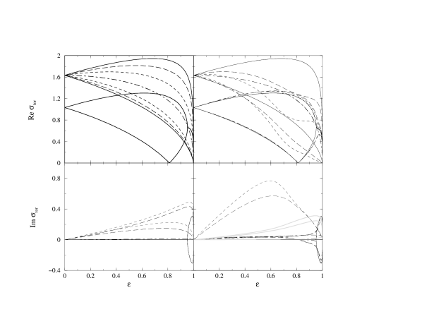
Figure 2: The CM and relative toroidal modes of superfluid Maclaurin spheroid. The imaginary parts shown in grey are magnified by factor 10. Other conventions are the same as in Fig. 1. Note the secular instability at the bifurcation point $\epsilon=0.81$ and the dynamical instability at the point $\epsilon=0.93$.

These equations can be manipulated to a set of four equations, which read

$$\left(\lambda^{2}+2f_{N}\nu\lambda+4B_{12}-2\Omega^{2}\right)V_{12}+\Omega\lambda(V_{11}-V_{22})$$ (171)

$$\hskip 113.81102pt-2f_{N}f_{S}\nu\lambda U_{12}=0,$$ (172)

$$\left(\lambda^{2}+2f_{N}\nu\lambda+4B_{12}-2\Omega^{2}\right)(V_{11}-V_{22})$$ (173)

$$\hskip 113.81102pt-4\Omega\lambda V_{12}-2f_{N}f_{S}\nu\lambda(U_{11}-U_{22})=0,$$ (174)

$$\left(\lambda^{2}+2\Omega\tilde{\beta}\lambda+2f_{S}\nu\lambda+4A_{1}-2\Omega^{2}\right)U_{12}$$ (175)

$$\hskip 113.81102pt+\Omega(1-\tilde{\beta}^{\prime})\lambda(U_{11}-U_{22})-2\nu\lambda V_{12}=0,$$ (176)

$$\left(\lambda^{2}+2\Omega\tilde{\beta}\lambda+2f_{S}\nu\lambda+4A_{1}-2\Omega^{2}\right)(U_{11}-U_{22})$$ (177)

$$\hskip 113.81102pt-4\Omega(1-\tilde{\beta}^{\prime})\lambda U_{12}-2\nu\lambda(V_{11}-V_{22})=0.$$ (178)

In the inviscid limit equations above decouple into separate sets for the CM and relative oscillations. The CM oscillations are described by the equations

$$\left(\lambda^{2}+4B_{12}-2\Omega^{2}\right)V_{12}+\Omega\lambda(V_{11}-V_{22})=0,$$ (179)

$$\left(\lambda^{2}+4B_{12}-2\Omega^{2}\right)(V_{11}-V_{22})-4\Omega\lambda V_{12}=0,$$ (180)

and their solutions are documented in EFE. The relative oscillations are described by the following equations

$$\left(\lambda^{2}+2\Omega\tilde{\beta}\lambda+4A_{1}-2\Omega^{2}\right)(U_{11}-U_{22})-4\Omega\lambda(1-\tilde{\beta}^{\prime})U_{12} = 0,$$ (181)

$$\ \left(\lambda^{2}+2\Omega\tilde{\beta}\lambda+4A_{1}-2\Omega^{2}\right)U_{12}+\Omega\lambda(1-\tilde{\beta}^{\prime})(U_{11}-U_{22}) = 0.$$ (182)

and the characteristic equation for the relative toroidal modes is:

$$\lambda^{4}+4\tilde{\beta}\Omega\lambda^{3}+(8A_{1}+4\tilde{\beta}^{2}\Omega^{2}-8\tilde{\beta}^{\prime}\Omega^{2}+4\tilde{\beta}^{\prime 2}\Omega^{2})\lambda^{2}$$ (183)

$$\hskip 56.9055pt+8\tilde{\beta}\Omega(2A_{2}-\Omega^{2})\lambda+4(2A_{1}-\Omega^{2})^{2}=0.$$ (184)

In the frictionless limit the modes can be found analytically from

$$(\lambda^{2}+4A_{1}-2\Omega^{2})^{2}+4\Omega^{2}\lambda^{2}=0,$$ (185)

which is factorized by writing $\lambda=i\sigma$. The two solutions are then

$$\sigma_{1,2}=\Omega\pm\sqrt{4A_{1}-\Omega^{2}}.$$ (186)

and there are two complementary modes which are found by substituting $-\Omega$ for $\Omega$. If the mutual friction is included the characteristic equation describing the relative oscillation modes is of order 4; in the presence of viscosity of the normal component, again the CM and relative oscillation modes couple and the characteristic equation is of order 8. The real and imaginary parts of the dissipative toroidal modes are shown in Fig. 2, for the same values of parameters as in Fig. 1. As for the transverse-shear modes, the CM and relative modes start at 1.03 and 1.63, respectively, when $\Omega\to 0$. In the inviscid limit (left panel), the CM modes are unaffected, as they should, while the relative modes are driven against each other and merge in the limit of strong coupling. The damping of the relative modes is finite, while for the CM modes it vanishes exactly up to the point of the onset of the dynamical instability at $\epsilon=0.95$; beyond this point a mode becomes dynamically (i.e. in the absence of dissipation) unstable. If the kinematic viscosity is finite (right panel), the real parts of the relative modes are strongly affected, while the effect of the viscosity on the CM modes is marginal. The imaginary part of a CM mode changes its sign at the bifurcation point, where $2B_{12}=\Omega^{2}$ and $\epsilon=0.813$. This signals the onset of the classical secular instability of the Maclaurin spheroid. The new feature here is that the mutual friction contributes to the secular instability of a CM-mode. On the other hand, ordinary viscosity does not drive the relative modes unstable, in agreement with the fact that there are no neutral points for these modes along the entire Maclaurin sequence. One may conclude that the agents which break the superfluid/normal fluid symmetry can not cause an instability of the relative modes. The only possibility that the relative modes become unstable is a shift of the balance between the kinetic and potential energy perturbations, which might occur for compressible fluids, e.g. polytrops. This problem will be studied elsewhere.

4.5 Pulsation mode ($l=2$, $m=0$)

Pulsation modes (or breathing modes) are the generalization of the radial pulsation modes of a sphere to the case of rotation. They correspond to $l=2$ and $m=0$ indexes in the expansion in spherical harmonics. The pulsation modes are determined by the full set of equations which are even in index 3. By suitable combination of the equations for the virials $V_{i;i}$, $V_{i;j}$, $U_{i;i}$ and $U_{i;j}$, where $i=1,2,3$ and $j=1,2$ the original set of equations can be reduced to

$$\left(\lambda^{2}/2+f_{N}\nu\lambda+4B_{11}-2B_{13}-\Omega^{2}\right)\left(V_{11}+V_{22}\right)$$ (187)

$$-\Bigl{[}\lambda^{2}+2f_{N}\nu(1-\gamma)\lambda+6B_{33}-2B_{13}\Bigr{]}V_{33}$$ (188)

$$+2\Omega\lambda(V_{1;2}-V_{2;1})-f_{N}f_{S}\nu\lambda(U_{11}+U_{22})+2f_{N}f_{S}\nu(1-\gamma)U_{33}=0,$$ (189)

$$\lambda^{2}(V_{1;2}-V_{2;1})-\Omega\lambda(V_{11}+V_{22})=0,$$ (190)

$$\left(\lambda^{2}/2+2A_{1}-\Omega^{2}+f_{S}\nu\lambda+\Omega\tilde{\beta}\lambda\right)(U_{11}+U_{22})$$ (191)

$$-\Bigl{[}\lambda^{2}+2\Omega\tilde{\beta}^{\prime\prime}\lambda+4A_{3}+2f_{S}\nu(1-\gamma)\lambda\Bigr{]}U_{33}$$ (192)

$$+2\Omega(1-\tilde{\beta}^{\prime})\lambda(U_{1;2}-U_{2;1})-\nu\lambda(V_{11}+V_{22})+2\nu(1-\gamma)\lambda V_{33}=0,$$ (193)

$$(\lambda^{2}+2\Omega\tilde{\beta}\lambda)(U_{1;2}-U_{2;1})-\Omega(1-\tilde{\beta}^{\prime})\lambda(U_{11}+U_{22})=0.$$ (194)

The characteristic equation is found by supplementing these equations by the divergence free constraint on the virials of the CM and relative motions:

$$\sum_{i=1}^{3}\frac{V_{ii}}{a_{i}^{2}}=0,\quad\sum_{i=1}^{3}\frac{U_{ii}}{a_{i}^{2}}=0.$$ (195)

An equivalent form of the divergence free constraint for Maclaurin spheroids can be written in terms of eccentricity, $(V_{11}+V_{22})(1-\epsilon^{2})+V_{33}=0$ and similarly for $U_{ii}$.

In absence of viscosity the equations above decouple into two independent sets for CM and relative oscillations. The CM oscillations are described by

$$\left(\lambda^{2}/2+4B_{11}-2B_{13}-\Omega^{2}\right)\left(V_{11}+V_{22}\right)$$ (196)

$$\hskip 56.9055pt-\Bigl{(}\lambda^{2}+6B_{33}-2B_{13}\Bigr{)}V_{33}+2\Omega\lambda(V_{1;2}-V_{2;1})=0,$$ (197)

$$\lambda^{2}(V_{1;2}-V_{2;1})-\Omega\lambda(V_{11}+V_{22})=0,$$ (198)

and coincide with the pulsation modes treated in EFE. The relative oscillation modes are defined by the equations

$$\left(\lambda^{2}/2+\Omega\tilde{\beta}\lambda-\Omega^{2}+2A_{1}\right)(U_{11}+U_{22})$$ (199)

$$\hskip 28.45274pt+2\Omega\lambda(1-\tilde{\beta}^{\prime})(U_{1;2}-U_{2;1})-(\lambda^{2}+4A_{3}+2\Omega\tilde{\beta}^{\prime\prime}\lambda)U_{33}=0,$$ (200)

$$\left(\lambda^{2}+2\Omega\tilde{\beta}\lambda\right)(U_{1;2}-U_{2;1})-\Omega\lambda(1-\tilde{\beta}^{\prime})(U_{11}+U_{22})=0,$$ (201)

which can be combined to:

$$\left[\left(\lambda^{2}+2\Omega\tilde{\beta}\lambda-2\Omega^{2}+4A_{1}\right)(\lambda^{2}+2\Omega\tilde{\beta}\lambda)+4\Omega^{2}\lambda^{2}(1-\tilde{\beta}^{\prime})^{2}\right](U_{11}+U_{22})$$ (203)

$$\hskip 56.9055pt-2\left[\left(\lambda^{2}+2\Omega\tilde{\beta}\lambda\right)\left(\lambda^{2}+2\Omega\lambda\tilde{\beta}^{\prime\prime}+4A_{3}\right)\right]U_{33}=0.$$

The modes are found by supplementing this equation by the divergence free condition (195). The third order characteristic equation in the inviscid limit is

$$(3-2\epsilon^{2})\lambda^{3}+[8\tilde{\beta}\Omega+4\tilde{\beta}^{\prime\prime}\Omega-4(\tilde{\beta}+\tilde{\beta}^{\prime\prime})\epsilon^{2}\Omega]\lambda^{2}+[4A_{1}+8(1-\epsilon^{2})A_{3}$$ (204)

$$\hskip 56.9055pt+2\Omega^{2}+4\tilde{\beta}^{2}\Omega^{2}-8\tilde{\beta}^{\prime}\Omega^{2}+4\tilde{\beta}^{\prime 2}\Omega^{2}+8(1-\epsilon^{2})\tilde{\beta}\tilde{\beta}^{\prime\prime}\Omega^{2}]\lambda$$ (205)

$$\hskip 56.9055pt+8A_{1}\tilde{\beta}\Omega+16(1-\epsilon^{2})A_{3}\tilde{\beta}\Omega-4\tilde{\beta}\Omega^{3}=0,$$ (206)

where the trivial mode $\lambda=0$ is neglected. In the frictionless limit we find ($\lambda=i\sigma$ as before)

$$\sigma=\pm\left[\frac{2\Omega^{2}+4A_{1}+8A_{3}(1-\epsilon^{2})}{(3-2\epsilon^{2})}\right]^{1/2}.$$ (207)

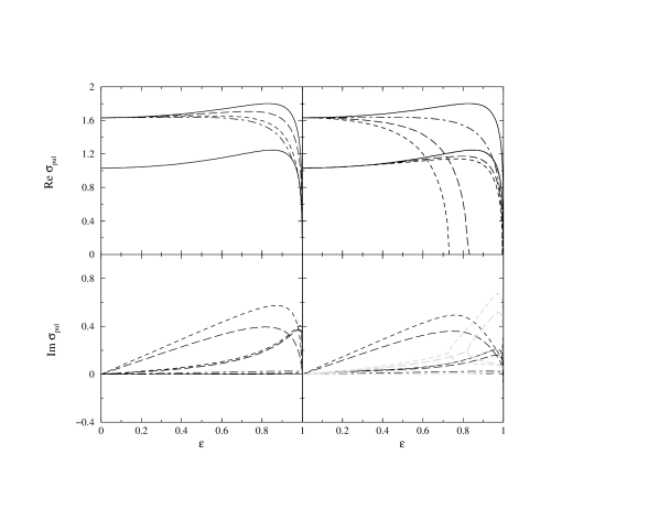
Figure 3: The CM and relative pulsation modes of superfluid Maclaurin spheroid. Conventions are the same as in Fig. 1 and 2.

The pulsation modes for a sphere follow in the limit ($\epsilon,\Omega)\to 0$: for a sphere $A_{i}/(\pi\rho G)=2/3$, and Eq. (207) reduces to $\sigma^{2}=8/3$ [$\sigma$ is given in units of $(\pi\rho G)^{1/2}$]. This result could be compared with the pulsation modes of an ordinary sphere: $\sigma^{2}=16/15$. Thus a superfluid sphere, apart form the ordinary pulsations, shows pulsations at frequencies roughly twice as large as the ordinary ones. In the general case where the viscosity of the normal fluid is taken into account the characteristic equation is of fifth order. The real and imaginary parts of the roots are shown in Fig. 3. In the inviscid limit the CM modes are again unaffected, while the relative modes are suppressed by the mutual friction. The damping of these modes is maximal when $\eta/\rho_{S}\omega=1$ and the motions correspond to stable, damped oscillations. In the presence of viscosity, the relative modes are strongly damped and eventually become neutral. The CM modes are weakly affected. The imaginary parts remain always positive, i.e. one finds stable, damped oscillations. Note that at the point where a relative pulsation mode becomes neutral the number of the imaginary components increases by one (as generally expected for the roots of polynomials), but there are no changes in the sign of the imaginary part of the neutral mode.

5 Summary

Let us briefly summarize the main qualitative features of the oscillations of superfluid self-gravitating systems SW2000 :

• The oscillation modes of the superfluid ellipsoids separate into two generic classes which correspond to co-moving and relative oscillations. The oscillation frequencies of these two classes have distinct values in the both slow and rapid rotation limits. The first class of oscillations is identical to those of classical single-fluid ellipsoids in the incompressible and inviscid limits. Corresponding modes are undamped if the Euler equations of fluids are symmetric/anti-symmetric with respect to the interchange $\alpha\leftrightarrow\beta$. When the fluids are coupled by mutual friction and mutual gravitational attraction this symmetry is preserved.

• The second class of oscillations, which is new, corresponds to relative motions of the fluids. The modes are damped by the mutual friction between the superfluid and the normal fluid. These modes correspond to stable oscillations.

• The co-moving (CM) modes emit gravitational radiation and undergo radiation reaction instabilities in full analogy to single-fluid ellipsoids GRAVRAD . The relative modes do not emit gravitational radiation at all, since the mass current associated with them is zero. This picture must hold true for a more general class of Chandrasekhar-Friedman-Schutz (CFS) radiation reaction instabilities, which are intrinsic to self-gravitating Newtonian fluids FS .

• If the $\alpha\leftrightarrow\beta$ symmetry is broken the two classes of modes mix, for example, when the normal fluid is viscous. The main effect of the mixing is the renormalization of the mutual friction and viscosity. The relative modes remain stable as there are no distinct neutral points for these modes along the ellipsoidal sequences. The CM modes become unstable at the classical points of onset of secular/dynamical instabilities, for example at the point of bifurcation of the Maclaurin spheroid into a Jacobi ellipsoid.

These qualitative features are based on general symmetries of underlying hydrodynamic equations and the conditions of equilibrium of self-gravitating fluids which are independent of the superfluid nature of underlying fluids (e.g. the existence of bifurcation points). Therefore we may conclude that these features will be preserved in more complex models of oscillations of superfluid neutron stars.

References

• (1) S. Chandrasekhar, E. Fermi: Astrophys. J. 118, 116 (1953)
• (2) S. Chandrasekhar, Ellipsoidal Figures of Equilibrium (Yale University Press, New Haven, 1969)
• (3) B. Carter, J. P. Luminet: Mon. Not. R. Astron. Soc. 212, 23, (1985); J. P. Luminet, B. Carter: Astrophys. J. Suppl. Ser. 61, 219 (1986)
• (4) J. R. Ipser, L. Lindblom: Astrophys. J., 355, 226 (1990); Astrophys. J., 379, 285 (1991); L. Lindblom, J. R. Ipser, Phys. Rev., D59 044009 (1999)
• (5) D. Lai, F. A. Rasio, S. L. Shapiro: Astrophys. J. Suppl. Ser. 88, 205 (1993)
• (6) S. L. Shapiro, S. A. Teukolsky, Black Holes, White Dwarfs and Neutrons Stars (Wiley, New York, 1983)
• (7) R. Epstein: Astrophys. J. 333, 880 (1988)
• (8) L. Lindblom, G. Mendell: Astrophys. J. 421, 689 (1994)
• (9) U. Lee: Astron. Astrophys. 303, 515 (1995)
• (10) L. Lindblom, G. Mendell: Phys. Rev. D61, 104003 (2000)
• (11) A. Sedrakian, I. Wasserman: Phys. Rev. D63, 024016 (2000)
• (12) I. M. Khalatnikov, Introduction to the Theory of Superfluidity (Addison Wesley, New York, 1989)
• (13) S. Chandrasekhar: Phys. Rev. Lett., 24, 611 (1970)
• (14) J. L. Friedman, B. F. Schutz: Astrophys. J., 221, 973 (1978)