Cosmic Shear Statistics and Cosmology

We report a measurement of cosmic shear correlations using an effective area of $6.5\leavevmode\nobreak\ sq.\leavevmode\nobreak\ deg.$ of the VIRMOS deep imaging survey in progress at the Canada-France-Hawaii Telescope. We measured various shear correlation functions, the aperture mass statistic and the top-hat smoothed variance of the shear with a detection significance exceeding $12\leavevmode\nobreak\ \sigma$ for each of them. We present results on angular scales from $3$ arc-seconds to half a degree. The consistency of different statistical measures is demonstrated and confirms the lensing origin of the signal through tests that rely on the scalar nature of the gravitational potential. For Cold Dark Matter models we find $\sigma_{8}\Omega_{0}^{0.6}=0.43^{+0.04}_{-0.05}$ at the $95\%$ confidence level. The measurement over almost three decades of scale allows to discuss the effect of the shape of the power spectrum on the cosmological parameter estimation. The degeneracy on $\sigma_{8}-\Omega_{0}$ can be broken if priors on the shape of the linear power spectrum (that can be parameterized by $\Gamma$) are assumed. For instance, with $\Gamma=0.21$ and at the $95\%$ confidence level, we obtain $0.6<\sigma_{8}<1.1$ and $0.2<\Omega_{0}<0.5$ for open models, and $\sigma_{8}>0.65$ and $\Omega_{0}<0.4$ for flat ($\Lambda$-CDM) models. From the tangential/radial modes decomposition we can set an upper limit on the intrinsic shape alignment, which was recently suggested as a possible contribution to the lensing signal. Within the error bars, there is no detection of intrinsic shape alignment for scales larger than $1^{\prime}$.

1 Introduction

Cosmological gravitational lensing produced by large-scale structure (or cosmic shear) has been advocated as a powerful tool to probe the mass distribution in the universe (see the reviews from Mellier (1999); Bartelmann & Schneider (2001) and references therein). The first detections reported over the past year (Van Waerbeke et al. (2000); Bacon et al. (2000); Kaiser et al. (2000); Wittman et al. (2000); Maoli et al. (2001); Rhodes et al. (2001)) confirmed that the amplitude and the shape of the signal are compatible with theoretical expectations, although the data sets were not large enough to place useful constraints on cosmological models. Maoli et al. (2001) combined the results from different groups to obtain constraints on the power spectrum normalization $\sigma_{8}$ and the mean density of the universe $\Omega_{0}$: Their result is in agreement with the cluster abundance constraints, but they were not yet able to break the degeneracy between $\sigma_{8}$ and $\Omega_{0}$.

The physical interpretation of the weak lensing signal can be made more securely using detections of cosmic shear from different statistics and angular scales on the same data set (as in Van Waerbeke et al. (2000)). Unfortunately, their joint detection of the variance and the correlation function using the same data was not fully conclusive: the sample was too small to enable a significant detection of the cosmic shear from variances with different weighting schemes and $2$-points statistics over a wide range of scales. The use of independent approaches is nevertheless necessary and it is a crucial step to validate the reliability of cosmic shear, to check the consistency of the measurements against theoretical predictions and to understand the residual systematics. A relevant example is the aperture mass statistic (defined in Schneider et al. (1998)). It is a direct probe of the projected mass power spectrum, and it is not sensitive to certain type of systematics (like a uniform PSF anisotropy) which may corrupt the top-hat smoothed variance, or the shear correlation function. Even the shear correlation function can be measured in several ways, by splitting the tangential and radial modes for instance.

In this paper we report the measurement of the top-hat smoothed variance, the aperture mass, the shear correlation function, and the tangential and radial shear correlation functions on a new homogeneous data set covering an effective area of 6.5 square-degrees (deg²). The depth and the field of view are well suited for a comprehensive analysis using various statistics. We show that the amplitude of residual systematics is very low compared to the signal and discuss the consistency of these measurements against the predictions of cosmological models.

We also discuss alternative interpretations. It has been suggested recently that intrinsic alignments of galaxies caused by tidal fields could contribute to the lensing signal (Croft & Metzler (2000); Heavens, Réfrégier & Heymans (2000); Catelan et al. (2000); Crittenden et al. 2000a ; Crittenden et al. 2000b ). This type of systematic is problematic because its signature on different $2$-points statistics mimics the lensing effect. A mode decomposition in electric and magnetic types (or $E$ and $B$ modes), similar to what is performed for the polarization analysis in the Cosmic Microwave Background, can separate lensing from intrinsic alignment (see Crittenden et al. 2000a ; Crittenden et al. 2000b ). The $E$ and $B$ mode analysis is the subject of a forthcoming paper; the aperture mass statistic presented in this paper is a similar analysis to the $E$ and $B$ mode decomposition, and allows us to put an upper limit on the contamination of our survey by the intrinsic alignments.

This paper is organized as follow: Section 2 describes our data set, and highlights the differences in the data preprocessing from our previous analysis (Van Waerbeke et al. (2000)). The measurement of the shear from this imaging data is discussed in Section 3. Section 4 summarizes the theoretical aspects of the different quantities we measure, and lists the statistical estimators used. The results and comparison to a few standard cosmological models are shown in Section 5. In Section 6 we perform a maximum likelihood analysis of cosmological models in the $(\Omega_{0},\sigma_{8})$ parameter space. The results on very small scales are shown separately in Section 7, and we conclude in Section 8.

2 The data set

The DESCART weak lensing project is a theoretical and observational program for cosmological weak lensing investigations. The cosmic shear survey carried out by the DESCART team uses the CFH12K data jointly with the VIRMOS survey to produce a large homogeneous photometric sample which will eventually contain a catalog of galaxies with redshifts as well as the projected mass density over the whole field (Le Fèvre et al (2001)). In contrast to Van Waerbeke et al. (2000), the new sample presented in this work only uses I-band data taken with the CFH12K camera and is therefore more homogeneous. It is worth noting that our new CFH12K sample only uses half of the data of the previous one. A comparison of the results will also permit to check the consistency and the robustness of the cosmic shear analysis.

The CFH12K data was obtained during dark nights in May 1999, November 1999 and April 2000 following the standard observation procedure described in Van Waerbeke et al (2000). The fields are spread over 4 independent $2\times 2$ deg² areas of the sky identified as F02, F10, F14 and F22. Each field is a compact mosaic of 16 CFH12K pointings named P[n]_n=1-16. Once the survey is completed each of them will cover 4 deg². Currently, of the final 16 deg², only 8.38 deg² is available for the analysis – most of the pointings are located in three different fields (F02, F10, F14 listed in Table 1). This total field of view gets significantly reduced by the masking and selection procedures described below. A summary of the data set characteristics are listed in Table 1.

Table 1: List of the fields. All observations were done in I band with the CFH12K camera (Cuillandre et al. (2000)). The number following the F denotes the field name, and the number following the P denotes the pointing name within the field. The geometry of the survey is detailed in http://terapix.iap.fr/Descart/. The image quality has been measured on each stacked image from a standard fitting of a Moffat profile.

Target	Used area	Exp. time	Period	Image quality
F02P1	980 ${\rm arcmin}^{2}$	9390 sec.	Nov. 1999	0.75”
F02P2	1078 ${\rm arcmin}^{2}$	7200 sec.	Nov. 1999	0.90”
F02P3	980 ${\rm arcmin}^{2}$	7200 sec.	Nov. 1999	0.90”
F02P4	1078 ${\rm arcmin}^{2}$	7200 sec.	Nov. 1999	0.80”
F10P1	882 ${\rm arcmin}^{2}$	3600 sec.	May 1999	0.65”
F10P2	882 ${\rm arcmin}^{2}$	3600 sec.	May 1999	0.75”
F10P3	490 ${\rm arcmin}^{2}$	3600 sec.	May 1999	0.75”
F10P4	882 ${\rm arcmin}^{2}$	3600 sec.	May 1999	0.65”
F10P5	882 ${\rm arcmin}^{2}$	3600 sec.	May 1999	0.75”
F10P7	1176 ${\rm arcmin}^{2}$	3600 sec.	Apr. 2000	0.75”
F10P8	1176 ${\rm arcmin}^{2}$	3600 sec.	Apr. 2000	0.70”
F10P9	98 ${\rm arcmin}^{2}$	3600 sec.	Apr. 2000	0.65”
F10P10	784 ${\rm arcmin}^{2}$	3600 sec.	Nov. 1999	0.80”
F10P11	294 ${\rm arcmin}^{2}$	3600 sec.	Nov. 1999/Apr. 2000	0.90”
F10P12	1176 ${\rm arcmin}^{2}$	3600 sec.	Apr. 2000	0.80”
F10P15	686 ${\rm arcmin}^{2}$	3600 sec.	Apr. 2000	0.85”
F14P1	882 ${\rm arcmin}^{2}$	3600 sec.	May 1999	0.80”
F14P2	882 ${\rm arcmin}^{2}$	3600 sec.	May 1999	0.85”
F14P3	686 ${\rm arcmin}^{2}$	3600 sec.	May 1999	0.75”
F14P4	1078 ${\rm arcmin}^{2}$	3600 sec.	May 1999	0.75”
F14P5	980 ${\rm arcmin}^{2}$	3600 sec.	May 1999	0.70”
F14P6	686 ${\rm arcmin}^{2}$	3600 sec.	May 1999	0.80”
F14P7	686 ${\rm arcmin}^{2}$	3600 sec.	May 1999	0.70”
F14P8	882 ${\rm arcmin}^{2}$	3600 sec.	May 1999	0.85”
F14P9	1078 ${\rm arcmin}^{2}$	3600 sec.	Apr. 2000	0.75”
F14P10	784 ${\rm arcmin}^{2}$	3600 sec.	May 1999	0.85”
F14P11	882 ${\rm arcmin}^{2}$	3600 sec.	Apr. 2000	0.80”
F14P12	784 ${\rm arcmin}^{2}$	3600 sec.	Apr. 2000	0.80”
F14P13	882 ${\rm arcmin}^{2}$	3600 sec.	Apr. 2000	0.85”
F14P14	882 ${\rm arcmin}^{2}$	3600 sec.	May 1999	1.0”
F14P15	882 ${\rm arcmin}^{2}$	3600 sec.	Apr. 2000	0.90”
F14P16	1176 ${\rm arcmin}^{2}$	2880 sec.	Apr. 2000	0.65”
F22P3	686 ${\rm arcmin}^{2}$	3600 sec.	May 1999	0.75”
F22P4	980 ${\rm arcmin}^{2}$	3600 sec.	Nov. 1999	0.75”
F22P6	588 ${\rm arcmin}^{2}$	3600 sec.	Apr. 2000	0.80”
F22P11	294 ${\rm arcmin}^{2}$	2880 sec.	Apr. 2000	0.75”

The data reduction was done at the TERAPIX data center. More than 1.5 Tbytes of data were processed in order to produce the final stacked images. The reduction procedure is the same as in Van Waerbeke et al. (2000), so we refer to this paper for the details. However, in order to improve the image quality prior to correction for the PSF anisotropy and to get a better signal-to-noise ratio on a larger angular scale than in our previous work, all CFH12K images were co-added after astrometric corrections.

The astrometric calibration and the co-addition were done using the MSCRED package in IRAF. Some tasks have been modified in order to allow a fully automatic usage of the package. For each pointing, we first started with the images in the I band. An astrometric solution was first found for one set of exposures in the dither sequence using the USNO-A 2.0 as reference, which provides the position of $\sim\times 10^{8}$ sources with an RMS accuracy of 0.3 arcsec. The astrometric solution was then transferred to the other exposures in the sequence. All object catalogs were obtained using SExtractor (Bertin & Arnouts (1996)) and a linear correction to the world coordinate system was computed with respect to the initial set. Finally, all images were resampled using a bi-cubic interpolation and then stacked together.

At this stage, each stacked image was inspected by eye and all areas which may potentially influence the later lensing analysis signal were masked (see Van Waerbeke et al. (2000) and Maoli et al. (2001)). Since we adopted conservative masks, this process had a dramatic impact on the field of view: we lost 20% of the total area and ended up with a usable area of 6.5 deg².

The photometric calibrations were done using standard stars from the Landolt’s catalog (Landolt (1992)) covering a broad sample of magnitude and colors. A full description of the photometric procedure is beyond the scope of this work and will be discussed elsewhere (Le Fèvre et al, in preparation). In summary, we used the SA110 and SA101 star fields to measure the zero-points and color equations of each run. From these calibrations, we produced the magnitude histograms of each field in order to find out the cut off and a rough limiting magnitude. Although few fields have exposure time significantly larger than 1 hour, the depth of the sample is reasonably stable from field to field and reaches $I_{AB}=24.5$. Up to this magnitude, 1.2 million galaxies were detected over the total area of 8.4 deg².

3 Shear measurements

3.1 Shape measurement

The details of our shape measurement procedure and Point Spread Function (hereafter PSF) correction have been extensively described in two previous papers (Van Waerbeke et al. (2000); Maoli et al. (2001)), and tested against numerical simulations (Erben et al. (2001)). Therefore we will not reproduce these details here, but only give a short overview of the procedure. The shape measurement pipeline uses the IMCAT software (Kaiser et al. (1995)) combined with the SExtractor package. The different steps in the procedure are as follows:

• Object detection with Sextractor.

• The shape parameters defined in Kaiser et al. (1995) are calculated using IMCAT.

• Stars are identified in the stellar branch of the size-magnitude diagram. Stars brighter than 1 magnitude below the saturation level are excluded. Objects smaller than the PSF size are discarded as galaxy candidates (because a shape correction below the PSF size is meaningless).

• The PSF is measured from the stars, and interpolated continuously over the CCD’s using a third order polynomial.

• Galaxy shapes are corrected using the scheme developed in Kaiser et al. (1995), modified and adapted to our problem as described in Erben et al. (2001). The shape correction is a two-step process: first we remove the anisotropic contribution of the PSF, then the isotropic contribution is suppressed according to Luppino & Kaiser (1997).

• A weight $w$ is calculated for each galaxy, which depends on the level of noise in the shape correction (see Eq.(7) in Van Waerbeke et al. (2000)).

• For each galaxy pair with members closer than 15 pixels (3 arcsec), one member is removed, in order to avoid the problem of overlapping isophotes reported in Van Waerbeke et al. (2000).

• Each CCD is visualized by eye, and the bad areas are masked (star spikes and ghost images, blank lines or columns, fringe residuals). After the whole process of cleaning and object selection, 420,000 galaxies were effectively used for the weak lensing analysis.

Figure 1: Top and third from the top panels: averaged $e^{\rm gal}_{1}$ and $e^{\rm gal}_{2}$ component versus the ellipticity of the PSF at the galaxy location, without the anisotropic PSF correction. Second from top and bottom panels: averaged $e^{\rm gal}_{1}$ and $e^{\rm gal}_{2}$ including the anisotropic PSF correction.

The raw ellipticity ${\bf e}$ of a galaxy is measured from the second moments $I_{ij}$ of the surface brightness $f({{\hbox{$\bf\theta$}}})$:

$${\bf e}=\left({I_{11}-I_{22}\over Tr(I)};{2I_{12}\over Tr(I)}\right),\ \ \ I_{ij}=\int{\rm d}^{2}\theta W(\theta)\theta_{i}\theta_{j}f({{\hbox{$\bf\theta$}}}).$$ (1)

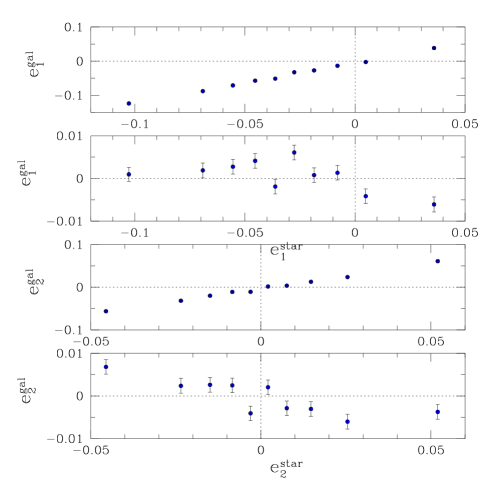
The window function $W({{\hbox{$\bf\theta$}}})$ suppresses the noise at large distances from the object center. The procedure described above gives a corrected galaxy ellipticity ${\bf e}^{\rm gal}$ calculated from the ${\bf e}$’s. According to Kaiser et al. (1995), the ensemble average of ${\bf e}^{\rm gal}$ is equal to the shear $\bf\gamma$ at the galaxy location. Figure 1 shows the level of systematics in ${\bf e}^{\rm gal}$ with and without the anisotropic PSF correction. After the PSF correction, the average galaxy ellipticity is bounded between $-0.005$ and $0.005$, and the variance of the residual systematics is less than $\sim 10^{-5}$. As we shall see later this is much less than the measured signal. As quoted in Van Waerbeke et al. (2000), the galaxy ellipticities show a small offset $(-0.008,-0.003)$, which has been corrected in this figure (the origin of this offset is still unclear). However it is worth to mention that the aperture mass is not sensitive to this offset.

4 Statistical measures of shear correlations

4.1 Theory

We summarize the different statistics we shall measure, and how they depend on cosmological models. We concentrate on 2-points statistics and variances, since higher order moments are more difficult to measure, and will be addressed in a forthcoming paper.

Let us assume a source redshift distribution parameterized as:

$$n(z_{s})={\beta\over z_{0}\ \Gamma\left({1+\alpha\over\beta}\right)}\left({z_{s}\over z_{0}}\right)^{\alpha}\exp\left[-\left({z_{s}\over z_{0}}\right)^{\beta}\right],$$ (2)

where the parameters $(z_{0},\alpha,\beta)=(0.8,2,1.5)$, which is consistent with a limiting magnitude $I_{AB}=24.5$ given by Cohen et al. (2000) (it corresponds to a mean redshift of $1.2$). We define the power spectrum of the convergence as (following the notation in Schneider et al. (1998)):

$$P_{\kappa}(k) = {9\over 4}\Omega_{0}^{2}\int_{0}^{w_{H}}{{\rm d}w\over a^{2}(w)}P_{3D}\left({k\over f_{K}(w)};w\right)\times$$ (3)

$$\int_{w}^{w_{H}}{\rm d}w^{\prime}n(w^{\prime}){f_{K}(w^{\prime}-w)\over f_{K}(w^{\prime})},$$

where $f_{K}(w)$ is the comoving angular diameter distance out to a distance $w$ ($w_{H}$ is the horizon distance), and $n(w(z))$ is the redshift distribution of the sources given in Eq.(2). $P_{3D}(k)$ is the non-linear mass power spectrum, and $k$ is the 2-dimensional wave vector perpendicular to the line-of-sight. For a top-hat smoothing window of radius $\theta_{c}$, the variance is:

$$\langle\gamma^{2}\rangle={2\over\pi\theta_{c}^{2}}\int_{0}^{\infty}\leavevmode\nobreak\ {{\rm d}k\over k}P_{\kappa}(k)[J_{1}(k\theta_{c})]^{2},$$ (4)

where $J_{1}$ is the first Bessel function of the first kind.
The aperture mass $M_{\rm ap}$ was introduced in Kaiser et al. (1994):

$$M_{\rm ap}=\int_{\theta<\theta_{c}}\leavevmode\nobreak\ {\rm d}^{2}{{\hbox{$\bf\theta$}}}\kappa({{\hbox{$\bf\theta$}}})\leavevmode\nobreak\ U(\theta),$$ (5)

where $\kappa({{\hbox{$\bf\theta$}}})$ is the convergence field, and $U(\theta)$ is a compensated filter (i.e. with zero mean). Schneider et al. (1998) applied this statistic to the cosmic shear measurements. They showed that the aperture mass variance is related to the convergence power spectrum by:

$$\langle M_{\rm ap}^{2}\rangle={288\over\pi\theta_{c}^{4}}\int_{0}^{\infty}\leavevmode\nobreak\ {{\rm d}k\over k^{3}}P_{\kappa}(k)[J_{4}(k\theta_{c})]^{2}.$$ (6)

$\langle M_{\rm ap}^{2}\rangle$ can be calculated directly from the shear $\bf\gamma$ without the need for a mass reconstruction.
For each galaxy, we define the tangential and radial shear components ($\gamma_{t}$ and $\gamma_{r}$) with respect to the center of the aperture:

$$\gamma_{t} = -\gamma_{1}\cos(2\phi)-\gamma_{2}\sin(2\phi)$$

$$\gamma_{r} = -\gamma_{2}\cos(2\phi)+\gamma_{1}\sin(2\phi),$$ (7)

where $\phi$ is the position angle between the x-axis and the line connecting the aperture center to the galaxy. It is then easy to show that the aperture mass is related to the tangential shear by:

$$M_{\rm ap}=\int_{\theta<\theta_{c}}\leavevmode\nobreak\ {\rm d}^{2}{{\hbox{$\bf\theta$}}}\gamma_{t}({{\hbox{$\bf\theta$}}})\leavevmode\nobreak\ Q(\theta),$$ (8)

where the filter $Q(\theta)$ is given from $U(\theta)$:

$$Q(\theta)={2\over\theta^{2}}\int_{0}^{\theta}\leavevmode\nobreak\ {\rm d}\theta^{\prime}\leavevmode\nobreak\ \theta^{\prime}\leavevmode\nobreak\ U(\theta^{\prime})-U(\theta)$$ (9)

If $\gamma_{t}$ is replaced by $\gamma_{r}$ in Eq.(8), then the lensing signal vanishes, due to the curl-free property of the shear field (Kaiser et al. (1994)). This remarkable property constitutes a test of the lensing origin of the signal. The change from $\gamma_{t}$ to $\gamma_{r}$ can simply be accomplished just by rotating the galaxies by $45$ degrees in the aperture (i.e. changing a curl-free field to a pure curl field). Hereafter we call the $M_{\rm ap}$ statistic measured with the 45 degrees rotated galaxies the $R$-mode ($R$ for radial mode), and $\langle M_{\perp}^{2}\rangle$ the corresponding variance. It is interesting to note that the $R$-mode is not expected to vanish if the measured signal is due to intrinsic alignments of galaxies (Crittenden et al. 2000b ). Therefore it can be used to constrain the amount of residual systematics as well as the degree of the intrinsic alignment of galaxies.
From the shear $\bf\gamma$ and its projections defined in Eq.(7) we can also define various galaxy pairwise correlation functions related to the convergence power spectrum. Note that the tangential and radial shear projections in what follows are performed using the relative location vector of the pair members, not from an aperture center. The following correlation functions can be defined (Miralda-Escudé (1991); Kaiser (1992)):

$$\langle\gamma\gamma\rangle_{\theta}={1\over 2\pi}\int_{0}^{\infty}\leavevmode\nobreak\ {\rm d}k\leavevmode\nobreak\ P_{\kappa}(k)J_{0}(k\theta),$$ (10)

$$\langle\gamma_{t}\gamma_{t}\rangle_{\theta}={1\over 2\pi}\int_{0}^{\infty}\leavevmode\nobreak\ {\rm d}k\leavevmode\nobreak\ P_{\kappa}(k)[J_{0}(k\theta)+J_{4}(k\theta)],$$ (11)

$$\langle\gamma_{r}\gamma_{r}\rangle_{\theta}={1\over 2\pi}\int_{0}^{\infty}\leavevmode\nobreak\ {\rm d}k\leavevmode\nobreak\ P_{\kappa}(k)[J_{0}(k\theta)-J_{4}(k\theta)],$$ (12)

where $\theta$ is the pair separation angle. The cross-correlation $\langle\gamma_{t}\gamma_{r}\rangle_{\theta}$ is expected to vanish for parity reasons (there is no preferred orientation on average).

It is easy to see that the Eqs.(4,6,10,11,12) are different ways to measure the same quantity, that is the convergence power spectrum $P_{\kappa}(k)$. Ultimately the goal is to deproject $P_{\kappa}(k)$ in order to reconstruct the 3D mass power spectrum from Eq.(3), but this is beyond the scope of this paper. Here we restrict our analysis to a joint detection of these statistics, and show that they are consistent with the gravitational lensing hypothesis. We will also examine the constraints on the power spectrum normalization $\sigma_{8}$ and the mean density of the universe $\Omega_{0}$.

4.2 Estimators

Let us now define the estimators we used to measure the quantities given in Eqs.(4,6,10,11,12).

The variance of the shear is simply obtained by a cell averaging of the squared shear $\gamma^{2}({{\hbox{$\bf\theta$}}}_{i})$ over the cell index $i$. An unbiased estimate of the squared shear for the cell $i$ is:

$$E[\gamma^{2}({{\hbox{$\bf\theta$}}}_{i})]={\displaystyle\sum_{\alpha=1}^{2}\sum_{k\neq l}^{N_{i}}w_{k}w_{l}\leavevmode\nobreak\ e^{\rm gal}_{\alpha}(\@vec{\theta}_{k})e^{\rm gal}_{\alpha}(\@vec{\theta}_{l})\over\displaystyle\sum_{k\neq l}^{N_{i}}w_{k}w_{l}},$$ (13)

where $w_{k}$ is the weight for the galaxy $k$, and $N_{i}$ is the number of galaxies in the cell $i$. The cell averaging over the survey is then an unbiased estimate of the shear variance $\langle\gamma^{2}\rangle$. However, due to the presence of masked areas (mentioned in Section 4.1), some cells may have a very low number of galaxies compared to others. Instead of applying an arbitrary sharp cut off on the fraction of the apertures filled with masks (as it was in previous works) we decided to keep all the cells, and to weight each of them with the squared sum of the galaxy weights located in the cell. The cell averaging is now defined as:

$$E[\gamma^{2}]={\displaystyle\sum_{\rm cells}\left[E[\gamma^{2}({{\hbox{$\bf\theta$}}}_{i})]\left(\sum_{k=1}^{N_{i}}w_{k}\right)^{2}\right]\over\displaystyle\sum_{\rm cells}\left[\left(\sum_{k=1}^{N_{i}}w_{k}\right)^{2}\right]},$$ (14)

where $i$ identifies the cell. One potential problem with this procedure is that the sum of the weights is related to the number of objects in the aperture, which is affected by magnification bias, and therefore correlated with the shear signal measured in the same aperture. Fortunately the first non-vanishing contribution of this weighting scheme is a third order effect (of order $1\%$), and is therefore negligible. The advantage is that we can use all cells without wondering about their filling factor, and it naturaly down-weights the cells which contain a large fraction of poorly determined galaxy ellipticities. The weighting scheme Eq.(14) has been tested against numerical simulation, using a simulated survey with exactly the same survey geometry as our data: it gave unbiased measures of the lensing signal applied to the galaxies.

The $M_{\rm ap}$ statistic is calculated from a similar estimator, although the smoothing window is no longer a top-hat but the $Q$ function defined in Eq.(9). An unbiased estimate of $M_{\rm ap}^{2}({{\hbox{$\bf\theta$}}}_{i})$ in the cell $i$ is:

$$E[M_{\rm ap}^{2}({{\hbox{$\bf\theta$}}}_{i})]={\displaystyle\sum_{k\neq l}^{N_{i}}w_{k}w_{l}\leavevmode\nobreak\ e^{\rm gal}_{t}(\@vec{\theta}_{k})e^{\rm gal}_{t}(\@vec{\theta}_{l})\leavevmode\nobreak\ Q(\theta_{k})Q(\theta_{l})\over\displaystyle\sum_{k\neq l}^{N}w_{k}w_{l}},$$ (15)

where $e_{t}^{\rm gal}$ is the tangential galaxy ellipticity, and $Q$ is given by (see Schneider et al. (1998)):

$$Q(\theta)={6\over\pi}\left({\theta\over\theta_{c}}\right)^{2}\left[1-\left({\theta\over\theta_{c}}\right)^{2}\right].$$ (16)

The estimation of $\langle M_{\rm ap}^{2}\rangle$ over the survey is then given by the same expression as in Eq.(14), with $E[\gamma^{2}({{\hbox{$\bf\theta$}}}_{i})]$ replaced by $E[M_{\rm ap}^{2}({{\hbox{$\bf\theta$}}}_{i})]$. We emphasize that the this filter probes effective scales $\theta_{c}/5$, and not $\theta_{c}$ (see Figure 2 in Schneider et al. (1998)). Therefore we have to be careful when comparing the signal at different scales between different estimators.

The shear correlation function $\langle\gamma\gamma\rangle_{\theta}$ at separation $\theta$ is obtained by identifying all the pairs of galaxies falling in the separation interval $[\theta-d\theta,\theta+d\theta]$, and calculating the pairwise shear correlation:

$$E[\gamma\gamma;\theta]={\displaystyle\sum_{\alpha=1}^{2}}{\displaystyle\sum_{pairs}w_{k}w_{l}\leavevmode\nobreak\ e^{\rm gal}_{\alpha}(\@vec{\theta}_{k})e^{\rm gal}_{\alpha}(\@vec{\theta}_{l})\over\displaystyle\sum_{pairs}w_{k}w_{l}}.$$ (17)

The tangential and radial correlation functions $\langle\gamma_{t}\gamma_{t}\rangle_{\theta}$ and $\langle\gamma_{r}\gamma_{r}\rangle_{\theta}$ are measured also from Eq.(17) by replacing ${\bf e}^{\rm gal}$ with $e_{t}^{\rm gal}$ and $e_{r}^{\rm gal}$ respectively and dropping the sum over $\alpha$. It is worth noting that the estimators given here are independent of the angular correlation properties of the source galaxies.

5 Results and comparison to cosmological models

Figure 2: Top-hat smoothed variance of the shear (points with error bars). The three models correspond to $(\Omega_{0},\Lambda,\sigma_{8})=(0.3,0,0.9),(0.3,0.7,0.9),(1,0,0.6)$ for the short-dashed, solid and long-dashed lines respectively. The power spectrum is a CDM-model with $\Gamma=0.21$. The error bars correspond to the dispersion of the variance measured from $200$ realizations of the data set with randomized orientations of the galaxy ellipticities.

Figure 3: The aperture mass statistic for the same models as in Figure 2. The lower panel plots the R-mode, obtained by making a 45 degree rotation as described in the text. There is no significant detection for $\theta>5\leavevmode\nobreak\ {\rm arcmin}$ (corresponding to an effective angular scale of $1^{\prime}$, as discussed in the text), which shows the low level of contamination by galaxy intrinsic alignment and/or residual systematics.

Figure 4: Shear correlation function $\langle\gamma\gamma\rangle_{\theta}$. The models are the same as in Figure 2. The lower panel uses a log-scale for the x-axis to highlight the small scale details.

Figure 5: Top panel: tangential shear correlation function $\langle\gamma_{t}\gamma_{t}\rangle_{\theta}$. Bottom panel: radial shear correlation function $\langle\gamma_{r}\gamma_{r}\rangle_{\theta}$. The models are the same as in Figure 2.

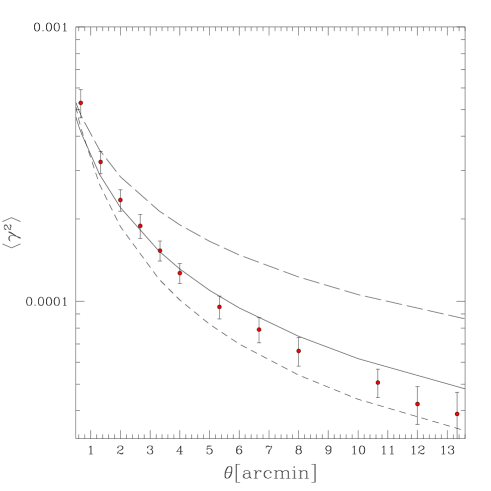
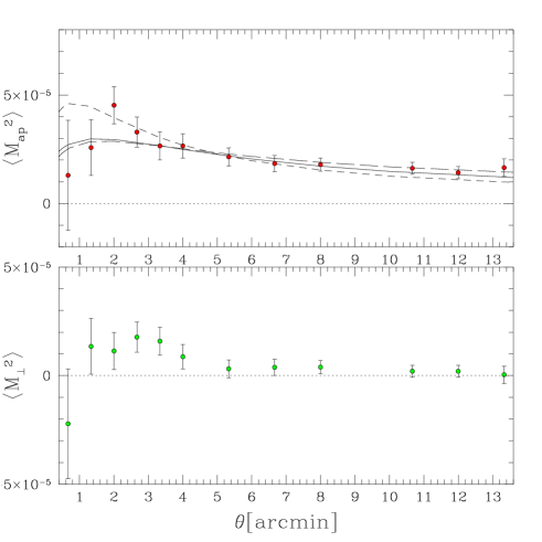
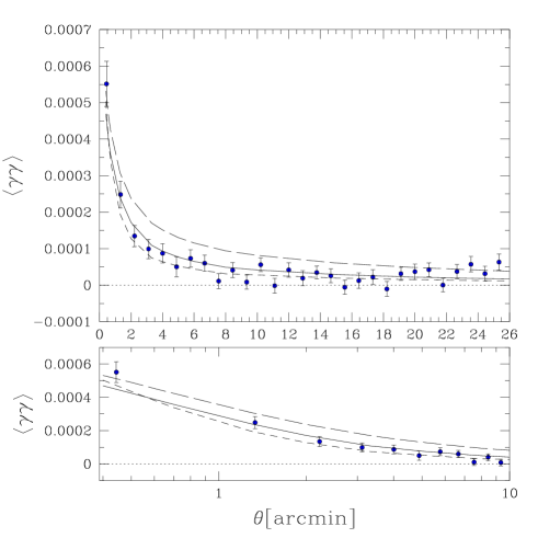
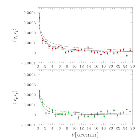
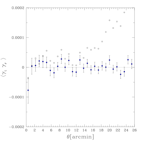
In this section we present our measurements of the 2-point correlations of the shear using the different estimators defined above. Figures 2 to 7 show the results for the different estimators: the variance in Figure 2, the mass aperture statistic in Figure 3, the shear correlation function in Figure 4, the radial and tangential shear correlations in Figure 5, and the cross-correlation of the radial and tangential shear in Figure 7. Along with the measurements we show the predictions of three cosmological models which are representative of an open model, a flat model with cosmological constant, and an Einstein-de Sitter model. The amplitude of mass fluctuations in these models is normalized to the abundance of galaxy clusters. The three models are characterized by the values of $\Omega_{0},\Lambda$ and $\sigma_{8}$ as follows:

• short-dashed line: $\Omega_{0}=0.3$, $\Lambda=0$, $\sigma_{8}=0.9$

• solid line: $\Omega_{0}=0.3$, $\Lambda=0.7$, $\sigma_{8}=0.9$

• long-dashed line: $\Omega_{0}=1$, $\Lambda=0$, $\sigma_{8}=0.6$

The power spectrum is taken to be a cold dark matter (CDM) power spectrum with shape parameter $\Gamma=0.21$. The predictions for shear correlations are computed using the non-linear evolution of the power spectrum using the Peacock & Dodds (1996) fitting formula. The source redshift distribution follows Eq.(2) with $(z_{0},\alpha,\beta)=(0.8,2,1.5)$, which corresponds to a mean redshift of 1.2.

It is reassuring that the different statistics agree with each other in their comparison with the model predictions. These statistics weight the data in different ways and are susceptible to different kinds of systematic errors. The consistency of all the 2-point estimators suggests that the level of systematics in the data is low compared to the signal. A further test for systematics is provided by measuring the cross-correlation function $\langle\gamma_{t}\gamma_{r}\rangle_{\theta}$, which should be zero for a signal due to gravitational lensing. Figure 7 shows the measured cross-correlation function, which is indeed consistent with zero on all scales. The figure also shows the cross-correlation obtained when the anisotropic contamination of the PSF is not corrected – clearly such a correction is crucial in measuring the lensing signal.

The lower panel of Figure 3 shows the R-mode of the mass aperture statistic. As this statistic uses a compensated filter, the scale beyond which the measured R-mode is consistent with zero ($5^{\prime}$ on the plot) corresponds to an effective angular scale $\theta\simeq 1^{\prime}$. This places an upper limit on measured shear correlations due to the intrinsic alignment of galaxies, given the redshift distribution of the sources. The vanishing of $\langle M_{\perp}^{2}\rangle$ for effective angular scales larger than $1^{\prime}$ strongly supports our conclusion that the level of residual systematics is low: this is a very hard test to pass, as it means that the signal is produced by a pure scalar field, which need not be the case for systematics. We checked that $M_{\perp}^{2}$ is Gaussian distributed with a zero average all over the survey, as what we would expect from a pure noise realisation. For scales below $5^{\prime}$ on the plot, the $R$-mode is not consistent with zero at the 2-$\sigma$ level. Since the cross-correlation $\langle\gamma_{t}\gamma_{r}\rangle_{\theta}$ is consistent with zero at this scale, the source of the $R$-mode is probably not a residual systematic. It might be due to the effect of intrinsic alignments (Crittenden et al. 2000b ), but it is difficult to be sure without further tests.

The error bars shown in Figures 2 to 7 are calculated from a measurement of the different statistics in $200$ realizations of the data set, with randomized orientations of the galaxies. We measured the sample variance from ray-tracing simulations (Jain et al. (2000)) and find that it is smaller than $20\%$ of the noise error bars shown here (see Van Waerbeke et al. (1999) where the sample variance has been calculated for surveys with similar geometry), therefore we have not included it in our figures. Figure 6 shows an estimate of the sample variance for the r.m.s. shear using a compact $6.5$ sq. degree ray-tracing simulation (Jain et al. (2000)). This figure shows that the sample variance is about order of magnitude smaller than the signal for the range of scales of interest. Hence our errors are not dominated by sample variance, as was the case in the first detections of cosmic shear. As the probed angular scales approach the size of the fields (which is $\sim 30^{\prime}$ with the CFH12K camera) the sample variance becomes larger. This could be responsible for the small fluctuations in the measured correlations in Figures 4 and 5 for scales larger than $24^{\prime}$.

Figure 6: Shear r.m.s. $\langle\gamma^{2}\rangle^{1/2}$ (solid line) measured in a ray-tracing simulation (Jain et al. (2000)) for the open $\Omega_{0}=0.3$ model. The dashed line is the sample variance of the shear r.m.s. measured from 7 different realisations of the mass distribution for a survey of $6.5$ sq. degrees.

Figure 7: Shear cross-correlation function $\langle\gamma_{t}\gamma_{r}\rangle_{\theta}$. The signal should vanish if the data are not contaminated by systematics. As a comparison, the open circles show the same cross-correlation function computed from the galaxy ellipticities where the anisotropic correction of the PSF has been skipped.

6 Cosmological constraints

As noted elsewhere (e.g. Bernardeau et al. (1997); Jain & Seljak (1997)), the parameters that dominate the 2-point shear statistics are the power spectrum normalization $\sigma_{8}$ and the mean density $\Omega_{0}$. We investigate below how the statistics measured in Figures 2 to 5 constrain these parameters. Our parameter estimates below rely on some simplifying assumptions; a more detailed analysis over a wider space of parameters will be presented elsewhere.

We assume that the data follow Gaussian statistics and neglect sample variance since it is a very small contributor to the noise for our survey, as discussed above. We compute the likelihood function $\cal L$:

$${\cal L}={1\over(2\pi)^{n/2}\left|{\bf S}\right|^{1/2}}\leavevmode\nobreak\ \exp{\left[-{1\over 2}\left({\rm{\bf d}-{\bf s}}\right)^{T}{\bf S}^{-1}\left({\rm{\bf d}-{\bf s}}\right)\right]},$$ (18)

where ${\bf d}$ and ${\bf s}$ are the data and model vectors respectively, and ${\bf S}:=\langle\left({\rm{\bf d}-{\bf s}}\right)^{T}\left({\rm{\bf d}-{\bf s}}\right)\rangle$ is the noise correlation matrix. ${\bf S}$ was computed for the different statistics from 200 random realizations of the survey, therefore effects associated with the survey geometry are included in our noise matrix. The model ${\bf s}$ was computed for a grid of cosmological models which covers $\Omega_{0}\in[0,1]$ and $\sigma_{8}\in[0.2,1.8]$ with a zero cosmological constant. The prior is chosen to be flat over this grid, and zero outside. We also fixed $\Gamma=0.21$ and used the redshift distribution of Eq.(2). We discuss below the impact of this choice of priors.

Figure 3 (bottom panel) shows that for effective scales smaller than $1^{\prime}$ there is a non-vanishing R-mode which could come either from a residual systematic, or from an intrinsic alignment effect. Therefore it is safer to exclude this part from the likelihood calculation. Thus for the top-hat variance, we excluded the point at $1^{\prime}$, for the correlation functions the points below $2^{\prime}$, and for the $M_{\rm ap}$ statistic the points below $5^{\prime}$. For the correlation function, we also excluded the points at scales larger than $20^{\prime}$ because of the small fluctuations in the measured correlations. The constraints on the cosmological parameters are not significantly affected whether these large scale points are excluded or not.

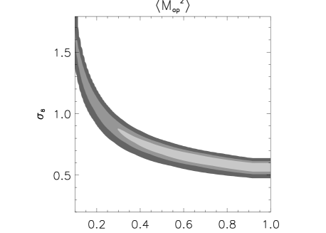
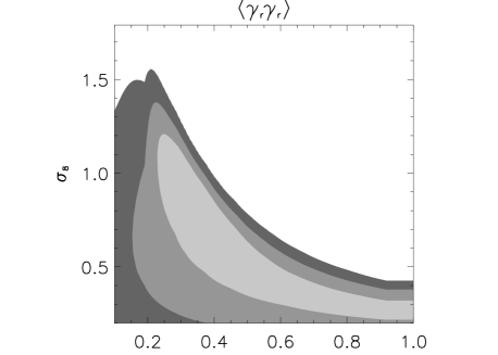
Figures 8 to 12 show the $(\Omega_{0},\sigma_{8})$ constraints for each of the statistics shown in Figures 2 to 5. The contours show the $99.9\%$, $95.0\%$ and $68.0\%$ confidence levels. The agreement between the contours is excellent, though the $M_{\rm ap}$ statistic and the radial correlation function do not give as tight constraints as the other statistics. The correlation function measurements below $2^{\prime}$ may be considered by using error bars that include a possible systematic bias: this is equivalent to adding a systematic covariance matrix ${\bf S}^{sys}$ to the noise covariance ${\bf S}$ matrix in Eq.(18). The new contours computed with the enlarged error bars are shown in Figure 13. The maximum of the likelihood in the variance and correlation function likelihood plots is at $\sigma_{8}\simeq 0.9$ and $\Omega_{0}\simeq 0.3$. Note that compared to a similar plot in Maoli et al. (2001) (Figure 8), here the contours are narrower, and are obtained from a homogeneous data set. Moreover, the degeneracy between $\Omega_{0}$ and $\sigma_{8}$ is broken.

The partial breaking of degeneracy between $\Omega_{0}$ and $\sigma_{8}$ was expected from the fully non-linear calculation of shear correlations (Jain & Seljak (1997)). In the non-linear regime the dependence of the $2$-points statistics on $\Omega_{0}$ and $\sigma_{8}$ becomes sensitive to angular scale. For example, as shown in Jain & Seljak (1997), the shear r.m.s. measures $\sigma_{8}\leavevmode\nobreak\ \Omega_{0}^{0.5}$ on scale between $2^{\prime}-5^{\prime}$, and $\sigma_{8}\leavevmode\nobreak\ \Omega_{0}^{0.8}$ on scales $\lower 2.15277pt\hbox{$\;\buildrel>\over{\sim}\;$}10^{\prime}$. Therefore a low $\Omega_{0}$ universe should see a net decrease of shear power at large scale compared to a $\Omega_{0}=1$ universe (for a given shape of the power spectrum), as evident in Figure 2. Note that the aperture mass $M_{\rm ap}$ is still degenerate with $\Omega_{0}$ and $\sigma_{8}$ (Figure 9) because it probes effective scales up to $\sim 2.6^{\prime}$ only, which is not enough to break the degeneracy.

It seems that the aperture mass (Figure 9) gives a slightly larger $\sigma_{8}$ for a large $\Omega_{0}$ compared to the other statistics, while they all agree for $\Omega_{0}<0.7$. This could be an indication for a low $\Omega_{0}$ Universe, however in practice, the probability contours for the different statistics cannot be combined in a straightforward way because they are largely redundant. The best strategy here is to concentrate on one particular statistic. We expect the best constraints from the shear correlation function (since it contains all the information by definition), and therefore base our parameter estimates on the likelihood contours obtained from it. The contours in the $\sigma_{8}-\Omega_{0}$ plane in Figure 13 closely follow the curve $\sigma_{8}\propto\Omega_{0}^{0.6}$. This allows us to obtain the following measurement of $\sigma_{8}\leavevmode\nobreak\ \Omega_{0}^{0.6}$ (from this figure alone):

$$\sigma_{8}\leavevmode\nobreak\ \Omega_{0}^{0.6}\ =\ 0.43^{+0.04(0.06)}_{-0.05(0.07)},$$ (19)

where the uncertainties correspond to the $95\%$ ($99.9\%$) confidence levels. The result in equation (19) is fairly robust against different values of $\Gamma$.

If we fix $\Gamma=0.21$, we can constrain the two parameters separately; we get, at the $95\%$ confidence level: $0.2<\Omega_{0}<0.5$ and $0.6<\sigma_{8}<1.1$ for open models and $\sigma_{8}>0.65$ and $\Omega_{0}<0.4$ for flat ($\Lambda$-CDM) models. This result however is sensitive to the prior choosen for $\Gamma$. In particular, if we use the relation $\Gamma=\Omega_{0}h$ for a cold dark matter model, then some extreme combinations of $\sigma_{8}$, $\Omega_{0}$ and $\Gamma$ cannot be ruled out from lensing alone. The degeneracy between $\Omega_{0}$ and $\sigma_{8}$ is broken only if we take $\Gamma$ to lie in a reasonable interval. Such interval can be motivated by galaxy surveys for instance, which give $0.19<\Gamma<0.37$ at $68\%$ confidence level for the APM (Eisentsein & Zaldarriaga (2001)). Therefore the separate constraints on $\Omega_{0}$ and $\sigma_{8}$ given above require some prior assumptions and must be taken with precaution, while the constraint on $\sigma_{8}\leavevmode\nobreak\ \Omega_{0}^{0.6}$ is much more robust. The redshift distribution of the sources is likely to be the main source of uncertainty in our estimate of equation (19); a rough guide is given by the scaling $\sigma_{8}\leavevmode\nobreak\ \Omega_{0}^{0.6}\propto z_{0}^{-0.5}$ (Jain & Seljak (1997)). A more detailed analysis of parameter estimation is left for a later study.

Figure 8: Likelihood contours in the $\Omega_{0}-\sigma_{8}$ plane from the top-hat smoothed variance $\langle\gamma^{2}\rangle$ shown in Figure 2. The first point in Figure 2 was not included in the likelihood calculation to avoid the small scale systematic shown in Figure 3 (bottom panel). The cosmological models have $\Lambda=0$, with a CDM-type power spectrum and $\Gamma=0.21$. The redshift of the sources is given by Eq.(2). with $(z_{0},\alpha,\beta)=(0.8,2,1.5)$. The confidence levels are $(0.68,0.95,0.999)$.

Figure 9: As in Figure 8, but using the $M_{\rm ap}$ statistic of (Figure 3, top panel) instead of the top-hat variance. The first five points in Figure 3 were not included in the likelihood calculation in order to avoid the small scale systematic shown in Figure 3 (bottom panel).

Figure 10: Likelihood contours as in Figure 8, but using the shear correlation function $\langle\gamma\gamma\rangle_{\theta}$ (Figure 4) instead of the top-hat variance. The first two points and scales larger than $20^{\prime}$ in Figure 4 were not included in the likelihood calculation to avoid the contribution from the small scale systematic shown in Figure 3 (bottom panel).

Figure 11: As in Figure 8, but using the tangential shear correlation function $\langle\gamma_{t}\gamma_{t}\rangle_{\theta}$ (Figure 5) instead of the top-hat variance. The first two points and scales larger than $20^{\prime}$ in Figure 5 were not included in the likelihood calculation in order to avoid the contribution from the small scale systematic shown in Figure 3 (bottom panel).

Figure 12: As in Figure 8, but using the radial shear correlation function $\langle\gamma_{r}\gamma_{r}\rangle_{\theta}$ (results in Figure 5) instead of the top-hat variance. The first two points and scales larger than $20^{\prime}$ in Figure 5 were not included in the likelihood calculation in order to avoid the contribution from the small scale systematic shown in Figure 3 (bottom panel).

Figure 13: Likelihood contours as in Figure 10, but all the points in Figure 4 on scales smaller than $20^{\prime}$ were used. In order to account for the small scale systematic shown in Figure 3 (bottom panel) the error bars on the first two points were increased to include the systematic amplitude.

7 Small scale signal

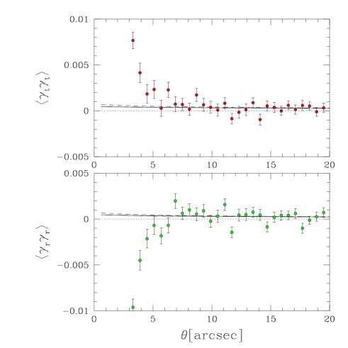
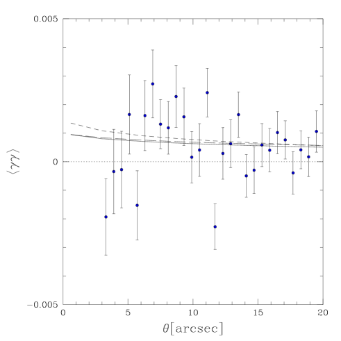
Our correlation function measurements extend to much smaller scales than shown in the figures above. The limit is set only by the fact that we reject one member of all pairs closer than $3$ arcsec. Figures 14 and 15 show the tangential, radial and total shear correlation functions. The pair separation bins are much smaller than in Figures 4 and 5, which explains why the error bars are larger. Even at the smallest scales, the shear correlation function $\langle\gamma\gamma\rangle_{\theta}$ is consistent with the model predictions.

The surprising result for the small scale correlations is the behavior of the tangential and radial shear correlation functions: at scales smaller than $5^{\prime\prime}$ we find an increased amplitude for $\langle\gamma_{t}\gamma_{t}\rangle_{\theta}$, and a ${\it negative}$ $\langle\gamma_{r}\gamma_{r}\rangle_{\theta}$. Though surprinsing, a negative $\langle\gamma_{r}\gamma_{r}\rangle_{\theta}$ is not unphysical: for instance in Kaiser (1992) (Table 1) a shallow mass power spectrum ($n>-1$) implies such an effect. In terms of halo mass profile, it corresponds to a projected profile steeper than $-1.5$. However, regardless of the nature of this signal, it is important to note that this is a very small scale effect which has no effect on the statistics discussed in preceding sections. The contribution of the increased signal from $\langle\gamma_{t}\gamma_{t}\rangle_{\theta}$ to the variance at $1^{\prime}$ is less than $1\%$; moreover since $\langle\gamma\gamma\rangle_{\theta}$ is not affected at all, the variance is also unaffected. As an explicit test, we checked that by removing one member of the pairs closer than $7^{\prime\prime}$ the measured signal in Figures 2,3,4,5 is unchanged. In a similar cosmic shear analysis using the Red-sequence Cluster Survey (Gladders & Yee (2000)) another group finds a similar small scale behavior, though at lower statistical significance (H. Hoekstra, private communication).

The cross-correlation $\langle\gamma_{t}\gamma_{r}\rangle_{\theta}$ vanishes down to $3^{\prime\prime}$, therefore no obvious systematic is responsible for this effect. The effect is unlikely to be caused by overlapping isophotes, or close neighbors effects because $\langle\gamma_{t}\rangle_{\theta}^{2}<<\langle\gamma_{t}\gamma_{t}\rangle_{\theta}$: if it were a close neighbor alignment we would expect that $\langle\gamma_{t}\rangle_{\theta}$ (the average tangential ellipticity for all the pair members in each pair separation bin $\theta$) carries all of the signal, which is not the case. In fact we find $\langle\gamma_{t}\rangle_{\theta}^{2}\sim 0.2\langle\gamma_{t}\gamma_{t}\rangle_{\theta}$, which means that close neighbor effect can hardly exceed $20\%$ of the small scale signal.

A forthcoming paper using the same data set will be devoted to the measurement of $E$ and $B$ modes (as defined in Crittenden et al. 2000a ), and we will study this small scale signal in more detail. At this stage of the analysis we cannot exclude a possible residual systematic. However, a preliminary analysis shows that the $B$ mode down to $3^{\prime\prime}$ is much smaller than the $E$ mode, which is hard to have if the signal comes from residual systematics.

Figure 14: Tangential (top panel) and radial (bottom panel) shear correlation functions $\langle\gamma_{t}\gamma_{t}\rangle_{\theta}$ and $\langle\gamma_{r}\gamma_{r}\rangle_{\theta}$ down to $3^{\prime\prime}$. The solid, long-dashed (hidden by the solid line) and short-dashed lines are predictions from the same models as in Figure 2.

Figure 15: Same as Figure 14 but for the shear correlation function $\langle\gamma\gamma\rangle_{\theta}$.

8 Conclusion

Using $6.5$ sq. deg. of the VIRMOS survey in progress at the CFHT, we were able to measure various $2$-points correlation statistics of cosmic shear. The top-hat variance, the aperture mass statistic and different shear correlation functions gave consistent results over a wide range of scales. Further tests of the lensing origin of the signal exploiting the scalar nature of the gravitational potential were also convincingly verified. We demonstrated that the level of systematics, in particular the intrinsic alignment of galaxies, is likely to be small, and does not contribute to the signal for scales larger than $1^{\prime}$. We believe that these results demonstrate the significance of our detection of shear correlations due to gravitational lensing. The quality of the data and the adequate size of our survey allow us to constrain cosmological models of the large-scale distribution of dark matter in the universe.

We have obtained tight constraints on the cosmological parameters $\Omega_{0}$ and $\sigma_{8}$. These results suggest that high precision measurements can be made with larger surveys on a much larger set of cosmological parameters. The final stage of the VIRMOS survey is to accomplish $16$ sq. deg. in patches of $4$ sq. deg., $4$ colors each, thus allowing the possibility to use the photometric redshifts of the galaxies. The use of photometric redshift will not only improve the scientific interpretation of cosmic shear (e.g. doing tomography as in Hu (1999)) but will be useful to measure the intrinsic alignment itself (which can be used to constrain galaxy formation models for instance).

The constraints obtained so far are within a framework of structure formation through gravitational instability with Gaussian initial conditions and Cold Dark Matter. As the amount of observations increases and the measurement quality improves, the first hints of the shape of the power spectrum will be soon available. It opens new means of really testing the formation mechanisms of the large-scale structure and the cosmological parameters beyond the standard model (Uzan & Bernardeau (2000)).

Over the last two years, we have seen the transition from the detection of the weak lensing signal to the first measurements of cosmological parameters from it. The agreement between theoretical predictions and observational results with such a high precision indicates that the measurement of cosmic shear statistics is becoming a mature cosmological tool. Many surveys are under way or scheduled for the next 5 years. They will use larger panoramic cameras than the CFH12K, and will cover solid angles 10 to 100 times wider than this work. The results of this work give us confidence that cosmic shear statistics will provide valuable measurements of cosmological parameters, probe the biasing of mass/light, produce maps of the dark matter distribution and reconstruct its power spectrum.