CMB Bispectrum from Active Models of Structure Formation

Abstract

We propose a new method for a numerical computation of the angular bispectrum of the CMB anisotropies arising from active models such as cosmic topological defects, using a modified Boltzmann code based on CMBFAST. The method does not use CMB sky maps and requires moderate computational power. As a first implementation, we apply our method to a recently proposed model of simulated cosmic strings and estimate the observability of the non-Gaussian bispectrum signal. A comparison with the cosmic variance of the bispectrum estimator shows that the bispectrum for the simulated string model we used is not observable.

]

Anisotropies of the Cosmic Microwave Background radiation (CMB) are directly related to the origin of structure in the universe. Galaxies and clusters of galaxies eventually formed by gravitational instability from primordial density fluctuations, and these same fluctuations left their imprint on the CMB. Recent balloon [1, 2] and ground-based interferometer [3] experiments have produced reliable estimates of the power spectrum of the CMB temperature anisotropies. While they helped eliminate certain candidate theories for the primary source of cosmic perturbations, the power spectrum data is still compatible with the theoretical estimates of a relatively large variety of models, such as $\Lambda$CDM, quintessence models or some hybrid models including cosmic defects. These models, however, differ in their predictions for the statistical distribution of the anisotropies beyond the power spectrum. Future MAP and Planck satellite missions (scheduled for launch in 2001 and 2007, respectively) will provide high-precision data allowing definite estimates of non-Gaussian signals in the CMB. It is therefore important to know precisely which are the predictions of all candidate models for the statistical quantities that will be extracted from the new data and identify their specific signatures.

There are two main classes of models of structure formation—passive and active models. In passive models, density inhomogeneities are set as initial conditions at some early time, and while they subsequently evolve as described by Einstein-Boltzmann equations, no additional perturbations are seeded. On the other hand, in active models the sources of density perturbations are time-dependent.

All specific realizations of passive models are based on the idea of inflation. In most inflationary models, density fluctuations arise from quantum fluctuations of a scalar field placed in the vacuum and hence are well described by a Gaussian distribution, while second-order effects may add a weak non-Gaussian signal [5].

On the other hand, active models of structure formation are motivated by cosmic topological defects. If our ideas about grand unification are correct, then some cosmic defects, such as domain walls, strings, monopoles or textures, should have formed during phase transitions in the early universe [6]. Once formed, cosmic strings could survive long enough to seed density perturbations. Defect models possess the attractive feature that they have no parameter freedom, as all the necessary information is in principle contained in the underlying particle physics model. Generically, perturbations produced by active models are not expected to be Gaussian distributed.

The narrow main peak and the presence of the second and the third peaks in the CMB angular power spectrum, as measured by BOOMERANG, MAXIMA and DASI [1, 2, 3], is an evidence for coherent oscillations of the photon-baryon fluid at the beginning of the decoupling epoch [7]. While such coherence is a property of all passive model, realistic cosmic string models produce highly incoherent perturbations that result in a much broader main peak. This excludes cosmic strings as the primary source of density fluctuations unless new physics is postulated, e.g. varying speed of light [8]. In addition to purely active or passive models, it has been recently suggested that perturbations could be seeded by some combination of the two mechanisms. For example, cosmic strings could have formed just before the end of inflation and partially contributed to seeding density fluctuations. It has been shown [9] that such hybrid models can be rather successful in fitting the CMB power spectrum data. Therefore, statistics beyond the power spectrum is required to discriminate between active and passive models.

Of the available non-Gaussian statistics, the CMB bispectrum, or the three-point function of Fourier components of the temperature anisotropy, has been perhaps the one best studied in the literature [10, 11]. Although there are a few cases where the bispectrum may be estimated analytically from the underlying model, a precise numerical code to compute it, similar to the CMBFAST code [12] for the power spectrum, is presently lacking. The bispectrum can be estimated from simulated CMB sky maps; however, computing a large number of full-sky maps resulting from defects is a much more demanding task.

In this article we introduce a new method for obtaining the CMB bispectrum directly from numerically simulated defect models, without building CMB sky maps. Given a suitable model, one can generate a statistical ensemble of realizations of defect matter perturbations. We use a modified Boltzmann code based on CMBFAST to compute the effect of these perturbations on the CMB and find the bispectrum estimator for a given realization of sources. We then perform statistical averaging over the ensemble of realizations to compute the expected CMB bispectrum. (The CMB power spectrum is also obtained as a byproduct.) Our method is specifically tailored for computations of the bispectrum; extending it to higher-order correlation functions would require prohibitively longer calculations. As a first application, we computed the expected CMB bispectrum from a model of simulated string networks first introduced by Albrecht et al. [13] and further developed in Ref. [14] and in this work. Our calculations indicate that the bispectrum resulting from this model is negligible when compared with the cosmic variance. We discuss the implications of this result for detectability of cosmic strings through the bispectrum statistic.

I CMB Bispectrum from active models

We assume that, given a model of active perturbations, such as a string simulation, we can calculate the energy-momentum tensor $T_{\mu\nu}({\mathbf{x}},\tau)$ for a particular realization of the sources in a finite spatial volume $V_{0}$. Here, ${\bf x}$ is a 3-dimensional coordinate and $\tau$ is the cosmic time. Many simulations are run to obtain an ensemble of random realizations of sources with statistical properties appropriate for the given model. The spatial Fourier decomposition of $T_{\mu\nu}$ can be written as

$$T_{\mu\nu}({{\mathbf{x}}},\tau)=\sum_{{\mathbf{k}}}\Theta_{\mu\nu}({{\mathbf{k}}},\tau)e^{i{{\mathbf{k}}}{{\mathbf{x}}}}\,\,\,,$$ (1)

where ${{\mathbf{k}}}$ are discrete. If $V_{0}$ is sufficiently large we can approximate the summation by the integral

$$\sum_{{\mathbf{k}}}\Theta_{\mu\nu}({{\mathbf{k}}},\tau)e^{i{{\mathbf{k}}}{{\mathbf{x}}}}\approx\frac{V_{0}}{(2\pi)^{3}}\int d^{3}{{\mathbf{k}}}\Theta_{\mu\nu}({{\mathbf{k}}},\tau)e^{i{{\mathbf{k}}}{{\mathbf{x}}}}\,\,\,,$$ (2)

and the corresponding inverse Fourier transform will be

$$\Theta_{\mu\nu}({{\mathbf{k}}},\tau)=\frac{1}{V_{0}}\int_{V_{0}}d^{3}{{\mathbf{x}}}\,T_{\mu\nu}({{\mathbf{x}}},\tau)e^{-i{{\mathbf{k}}}{{\mathbf{x}}}}\,\,\,.$$ (3)

Of course, the final results, such as the CMB power spectrum or bispectrum, do not depend on the choice of $V_{0}$. To ensure this independence, we shall keep $V_{0}$ in all expressions where it appears throughout the following sections.

It is conventional to expand the temperature fluctuations over the basis of spherical harmonics,

$${\Delta T/T}({\hat{{\mathbf{n}}}})=\sum_{lm}a_{lm}Y_{lm}({\hat{{\mathbf{n}}}}),$$ (4)

where $\hat{{\mathbf{n}}}$ is a unit vector. The coefficients $a_{lm}$ can be decomposed into Fourier modes,

$$a_{lm}=\frac{V_{0}}{(2\pi)^{3}}\left(-i\right)^{l}4\pi\int d^{3}{{\mathbf{k}}}\,\Delta_{l}\left({{\mathbf{k}}}\right)Y^{*}_{lm}({\hat{{\mathbf{k}}}}).$$ (5)

Given the sources $\Theta_{\mu\nu}({{\mathbf{k}}},\tau)$, the quantities $\Delta_{l}({{\mathbf{k}}})$ are found by solving linearized Einstein-Boltzmann equations and integrating along the line of sight, using a code similar to CMBFAST [12]. This standard procedure can be written symbolically as the action of a linear operator ${\hat{B}}_{l}^{\mu\nu}(k)$ on the source energy-momentum tensor, $\Delta_{l}({{\mathbf{k}}})={\hat{B}}_{l}^{\mu\nu}(k)\Theta_{\mu\nu}({{\mathbf{k}}},\tau)$, so the third moment of $\Delta_{l}({{\mathbf{k}}})$ is linearly related to the three-point correlator of $\Theta_{\mu\nu}({{\mathbf{k}}},\tau)$. Below we consider the quantities $\Delta_{l}({{\mathbf{k}}})$, corresponding to a set of realizations of active sources, as given. The numerical procedure for computing $\Delta_{l}({{\mathbf{k}}})$ was developed in Refs. [13] and [14].

The third moment of $a_{lm}$, namely $\left\langle a_{l_{1}m_{1}}a_{l_{2}m_{2}}a_{l_{3}m_{3}}\right\rangle$, can be expressed as

$$\left(-i\right)^{l_{1}+l_{2}+l_{3}}\left(4\pi\right)^{3}\!\!\frac{V_{0}^{3}}{(2\pi)^{9}}\!\!\int\!\!d^{3}{{\mathbf{k}}}_{1}d^{3}{{\mathbf{k}}}_{2}d^{3}{{\mathbf{k}}}_{3}Y^{*}_{l_{1}m_{1}}\!({\hat{{\mathbf{k}}}}_{1})$$ (6)

$$\times Y^{*}_{l_{2}m_{2}}\!({\hat{{\mathbf{k}}}}_{2})Y^{*}_{l_{3}m_{3}}\!({\hat{{\mathbf{k}}}}_{3})\left\langle\Delta_{l_{1}}\!\!\left({{\mathbf{k}}}_{1}\right)\Delta_{l_{2}}\!\!\left({{\mathbf{k}}}_{2}\right)\Delta_{l_{3}}\!\!\left({{\mathbf{k}}}_{3}\right)\right\rangle.$$ (7)

A straightforward numerical evaluation of Eq. (7) from given sources $\Delta_{l}\left({{\mathbf{k}}}\right)$ is prohibitively difficult, because it involves too many integrations of oscillating functions. However, we shall be able to reduce the computation to integrations over scalars (a similar method was employed in [15]). Due to homogeneity, the 3-point function vanishes unless the triangle constraint is satisfied,

$${{\mathbf{k}}}_{1}+{{\mathbf{k}}}_{2}+{{\mathbf{k}}}_{3}=0.$$ (8)

We may write

$$\left\langle\Delta_{l_{1}}\left({{\mathbf{k}}}_{1}\right)\Delta_{l_{2}}\left({{\mathbf{k}}}_{2}\right)\Delta_{l_{3}}\left({{\mathbf{k}}}_{3}\right)\right\rangle$$ (9)

$$= \delta^{(3)}\left({{\mathbf{k}}}_{1}+{{\mathbf{k}}}_{2}+{{\mathbf{k}}}_{3}\right)P_{l_{1}l_{2}l_{3}}\left({{\mathbf{k}}}_{1},{{\mathbf{k}}}_{2},{{\mathbf{k}}}_{3}\right),$$ (10)

where the three-point function $P_{l_{1}l_{2}l_{3}}\left({{\mathbf{k}}}_{1},{{\mathbf{k}}}_{2},{{\mathbf{k}}}_{3}\right)$ is defined only for values of ${\mathbf{k}}_{i}$ that satisfy Eq. (8). Given the scalar values $k_{1}$, $k_{2}$, $k_{3}$, there is a unique (up to an overall rotation) triplet of directions ${\hat{{\mathbf{k}}}}_{i}$ for which the RHS of Eq. (10) does not vanish. The quantity $P_{l_{1}l_{2}l_{3}}\left({{\mathbf{k}}}_{1},{{\mathbf{k}}}_{2},{{\mathbf{k}}}_{3}\right)$ is invariant under an overall rotation of all three vectors ${{\mathbf{k}}}_{i}$ and therefore may be equivalently represented by a function of scalar values $k_{1}$, $k_{2}$, $k_{3}$, while preserving all angular information. Hence, we can rewrite Eq. (10) as

$$\left\langle\Delta_{l_{1}}\!\!\left({{\mathbf{k}}}_{1}\right)\Delta_{l_{2}}\!\!\left({{\mathbf{k}}}_{2}\right)\Delta_{l_{3}}\!\!\left({{\mathbf{k}}}_{3}\right)\right\rangle$$ (11)

$$= \delta^{(3)}\left({{\mathbf{k}}}_{1}+{{\mathbf{k}}}_{2}+{{\mathbf{k}}}_{3}\right)P_{l_{1}l_{2}l_{3}}(k_{1},k_{2},k_{3}).$$ (12)

Then, using the simulation volume $V_{0}$ explicitly, we have

$$P_{l_{1}l_{2}l_{3}}\!\left(k_{1},k_{2},k_{3}\right)\!=\!\frac{(2\pi)^{3}}{V_{0}}\left\langle\Delta_{l_{1}}\!\!\left({{\mathbf{k}}}_{1}\right)\Delta_{l_{2}}\!\!\left({{\mathbf{k}}}_{2}\right)\Delta_{l_{3}}\!\!\left({{\mathbf{k}}}_{3}\right)\right\rangle.$$ (13)

Given an arbitrary direction $\hat{{\mathbf{k}}}_{1}$ and the magnitudes $k_{1}$, $k_{2}$ and $k_{3}$, the directions $\hat{{\mathbf{k}}}_{2}$ and $\hat{{\mathbf{k}}}_{3}$ are specified up to overall rotations by the triangle constraint. Therefore, both sides of Eq. (13) are functions of scalar $k_{i}$ only. The expression on the RHS of Eq. (13) is evaluated numerically by averaging over different realizations of the sources and over permissible directions $\hat{{\mathbf{k}}}_{i}$; below we shall give more details of the procedure.

Substituting Eqs. (12) and (13) into (7), Fourier transforming the Dirac delta and using the Rayleigh identity, we can perform all angular integrations analytically and obtain a compact form for the third moment,

$$\left\langle a_{l_{1}m_{1}}a_{l_{2}m_{2}}a_{l_{3}m_{3}}\right\rangle={\mathcal{H}}_{l_{1}l_{2}l_{3}}^{m_{1}m_{2}m_{3}}\int r^{2}dr\,b_{l_{1}l_{2}l_{3}}(r),$$ (14)

where, denoting the Wigner $3j$-symbol by $\left({}^{\,\,l_{1}\,\;l_{2}\,\;l_{3}}_{m_{1}m_{2}m_{3}}\right)$, we have

$${\mathcal{H}}_{l_{1}l_{2}l_{3}}^{m_{1}m_{2}m_{3}} \equiv \sqrt{\frac{\left(2l_{1}+1\right)\left(2l_{2}+1\right)\left(2l_{3}+1\right)}{4\pi}}$$ (20)

$$\times\left(\begin{array}[]{ccc}l_{1}&l_{2}&l_{3}\\ 0&0&0\end{array}\right)\left(\begin{array}[]{ccc}l_{1}&l_{2}&l_{3}\\ m_{1}&m_{2}&m_{3}\end{array}\right)\,,$$

and where we have defined the auxiliary quantities $b_{l_{1}l_{2}l_{3}}$ using spherical Bessel functions $j_{l}$,

$$b_{l_{1}l_{2}l_{3}}(r) \equiv \frac{8}{\pi^{3}}\frac{V_{0}^{3}}{(2\pi)^{3}}\int k_{1}^{2}dk_{1}\,k_{2}^{2}dk_{2}\,k_{3}^{2}dk_{3}\,$$ (21)

$$\times j_{l_{1}}(k_{1}r)j_{l_{2}}(k_{2}r)j_{l_{3}}(k_{3}r)P_{l_{1}l_{2}l_{3}}(k_{1},k_{2},k_{3}).$$ (22)

The volume factor $V_{0}^{3}$ contained in this expression is correct: as shown in the next section, each term $\Delta_{l}$ includes a factor $V_{0}^{-2/3}$, while the average quantity $P_{l_{1}l_{2}l_{3}}(k_{1},k_{2},k_{3})\propto V_{0}^{-3}$ [cf. Eq. (13)], so that the arbitrary volume $V_{0}$ of the simulation cancels.

Our proposed numerical procedure therefore consists of computing the RHS of Eq. (14) by evaluating the necessary integrals. For fixed $\left\{l_{1}l_{2}l_{3}\right\}$, computation of the quantities $b_{l_{1}l_{2}l_{3}}(r)$ is a triple integral over scalar $k_{i}$ defined by Eq. (22); it is followed by a fourth scalar integral over $r$ [Eq. (14)]. We also need to average over many realizations of sources to obtain $P_{l_{1}l_{2}l_{3}}\!\left(k_{1},k_{2},k_{3}\right)$. It was not feasible for us to precompute the values $P_{l_{1}l_{2}l_{3}}\!\left(k_{1},k_{2},k_{3}\right)$ on a grid before integration because of the large volume of data: for each set $\left\{l_{1}l_{2}l_{3}\right\}$ the grid must contain $\sim 10^{3}$ points for each $k_{i}$. Instead, we precompute $\Delta_{l}\!\!\left({{\mathbf{k}}}\right)$ from one realization of sources and evaluate the RHS of Eq. (13) on that data as an estimator of $P_{l_{1}l_{2}l_{3}}\!\left(k_{1},k_{2},k_{3}\right)$, averaging over allowed directions of $\hat{{\mathbf{k}}}_{i}$. The result is used for integration in Eq. (22).

Because of isotropy and since the allowed sets of directions $\hat{{\mathbf{k}}}_{i}$ are planar, it is enough to restrict the numerical calculation to directions $\hat{{\mathbf{k}}}_{i}$ within a fixed two-dimensional plane. This significantly reduces the amount of computations and data storage, since $\Delta_{l}\!\left({{\mathbf{k}}}\right)$ only needs to be stored on a two-dimensional grid of ${\mathbf{k}}$.

In estimating $P_{l_{1}l_{2}l_{3}}\!\left(k_{1},k_{2},k_{3}\right)$ from Eq. (13), averaging over directions of $\hat{{\mathbf{k}}}_{i}$ plays a similar role to ensemble averaging over source realizations. Therefore if the number of directions is large enough (we used 720 for cosmic strings), only a moderate number of different source realizations is needed. The main numerical difficulty is the highly oscillating nature of the function $b_{l_{1}l_{2}l_{3}}(r)$. The calculation of the bispectrum for cosmic strings presented in Section II requires about 20 days of a single-CPU workstation time per realization.

We note that this method is specific for the bispectrum and cannot be applied to compute higher-order correlations. The reason is that higher-order correlations involve configurations of vectors ${\mathbf{k}}_{i}$ that are not described by scalar values $k_{i}$ and not restricted to a plane. For instance, a computation of a 4-point function would involve integration of highly oscillating functions over four vectors ${\mathbf{k}}_{i}$ which is computationally infeasible.

From Eq. (14) we derive the CMB angular bispectrum ${\mathcal{C}}_{l_{1}l_{2}l_{3}}$, defined as[16]

$$\bigl{\langle}a_{l_{1}m_{1}}a_{l_{2}m_{2}}a_{l_{3}m_{3}}\bigr{\rangle}=\left(\begin{array}[]{ccc}l_{1}&l_{2}&l_{3}\\ m_{1}&m_{2}&m_{3}\end{array}\right){\mathcal{C}}_{l_{1}l_{2}l_{3}}\,.$$ (25)

The presence of the 3$j$-symbol guarantees that the third moment vanishes unless $m_{1}+m_{2}+m_{3}=0$ and the $l_{i}$ indices satisfy the triangle rule $|l_{i}-l_{j}|\leq l_{k}\leq l_{i}+l_{j}$. Invariance under spatial inversions of the three-point correlation function implies the additional ‘selection rule’ $l_{1}+l_{2}+l_{3}=\mbox{even}$, in order for the third moment not to vanish. Finally, from this last relation and using standard properties of the 3$j$-symbols, it follows that the angular bispectrum ${\mathcal{C}}_{l_{1}l_{2}l_{3}}$ is left unchanged under any arbitrary permutation of the indices $l_{i}$.

In this paper we restrict our calculations to the angular bispectrum $C_{l_{1}l_{2}l_{3}}$ in the ‘diagonal’ case, i.e. $l_{1}=l_{2}=l_{3}=l$. This is a representative case and, in fact, the one most frequently considered in the literature. Plots of the power spectrum are usually done in terms of $l(l+1)C_{l}$ which, apart from constant factors, is the contribution to the mean squared anisotropy of temperature fluctuations per unit logarithmic interval of $l$. In full analogy with this, the relevant quantity to work with in the case of the bispectrum is

$$G_{lll}=l(2l+1)^{3/2}\left(\begin{array}[]{ccc}l&l&l\\ 0&0&0\end{array}\right)C_{lll}\,.$$ (28)

Details of this derivation are presented in the Appendix. For large values of the multipole index $l$, $G_{lll}\propto l^{3/2}C_{lll}$. Note also what happens with the 3$j$-symbols appearing in the definition of the coefficients ${\mathcal{H}}_{l_{1}l_{2}l_{3}}^{m_{1}m_{2}m_{3}}$: the symbol $\left({}^{\,\,l_{1}\,\;l_{2}\,\;l_{3}}_{m_{1}m_{2}m_{3}}\right)$ is absent from the definition of $C_{l_{1}l_{2}l_{3}}$, while in Eq. (28) the symbol $\left({}^{\,l\;l\;l}_{0\>0\>0}\right)$ is squared. Hence, there are no remnant oscillations due to the alternating sign of $\left({}^{\,l\;l\;l}_{0\>0\>0}\right)$.

However, even more important than the value of $C_{lll}$ itself is the relation between the bispectrum and the cosmic variance associated with it. In fact, it is their comparison that tells us about the observability ‘in principle’ of the non-Gaussian signal. The cosmic variance constitutes a theoretical uncertainty for all observable quantities and comes about due to the fact of having just one realization of the stochastic process, in our case, the CMB sky [17].

The way to proceed is to employ an estimator $\hat{C}_{l_{1}l_{2}l_{3}}$ for the bispectrum and compute the variance from it. By choosing an unbiased estimator we ensure it satisfies $C_{l_{1}l_{2}l_{3}}=\langle\hat{C}_{l_{1}l_{2}l_{3}}\rangle$. However, this condition does not isolate a unique estimator. The proper way to select the best unbiased estimator is to compute the variances of all candidates and choose the one with the smallest value. The estimator with this property was computed in Ref. [16] and is

$$\hat{C}_{l_{1}l_{2}l_{3}}=\!\!\!\sum_{m_{1},m_{2},m_{3}}\!\!\left(\begin{array}[]{ccc}l_{1}&l_{2}&l_{3}\\ m_{1}&m_{2}&m_{3}\end{array}\right)a_{l_{1}m_{1}}a_{l_{2}m_{2}}a_{l_{3}m_{3}}.$$ (29)

The variance of this estimator, assuming a mildly non-Gaussian distribution, can be expressed in terms of the angular power spectrum $C_{l}$ as follows [11]

$$\sigma^{2}_{\hat{C}_{l_{1}l_{2}l_{3}}}\!\!\!\!=C_{l_{1}}C_{l_{2}}C_{l_{3}}\!\left(1\!+\!\delta_{l_{1}l_{2}}\!\!+\!\delta_{l_{2}l_{3}}\!\!+\!\delta_{l_{3}l_{1}}\!\!+\!2\delta_{l_{1}l_{2}}\delta_{l_{2}l_{3}}\right).$$ (30)

The theoretical signal-to-noise ratio for the bispectrum is then given by

$$(S/N)_{l_{1}l_{2}l_{3}}=|C_{l_{1}l_{2}l_{3}}/\sigma_{\hat{C}_{l_{1}l_{2}l_{3}}}|.$$ (31)

In turn, for the diagonal case $l_{1}=l_{2}=l_{3}=l$ we have

$$(S/N)_{l}=|C_{lll}/\sigma_{\hat{C}_{lll}}|.$$ (32)

Incorporating all the specifics of the particular experiment, such as sky coverage, angular resolution, etc., will allow us to give an estimate of the particular non-Gaussian signature associated with a given active source and, if observable, indicate the appropriate range of multipole $l$’s where it is best to look for it.

II Bispectrum from strings

A The string model

To calculate the sources of perturbations we use an updated version of the cosmic string model first introduced by Albrecht et al. [13] and further developed in Ref. [14], where the wiggly nature of strings was taken into account. In these previous works the model was tailored to the computation of the two-point statistics (matter and CMB power spectra). When dealing with higher-order statistics, such as the bispectrum, a different strategy needs to be employed.

In the model, the string network is represented by a collection of uncorrelated straight string segments produced at some early epoch and moving with random uncorrelated velocities. At every subsequent epoch, a certain fraction of the number of segments decays in a way that maintains network scaling. The length of each segment at any time is taken to be equal to the correlation length of the network. This and the root mean square velocity of segments are computed from the velocity-dependent one-scale model of Martins and Shellard [18]. The positions of segments are drawn from a uniform distribution in space, and their orientations are chosen from a uniform distribution on a two-sphere.

The total energy of the string network in a volume $V$ at any time is $E=N\mu L$, where $N$ is the total number of string segments at that time, $\mu$ is the mass per unit length, and $L$ is the length of one segment. If $L$ is the correlation length of the string network then, according to the one-scale model, the energy density is $\rho={E/V}={\mu/L^{2}}$, where $V=V_{0}a^{3}$, the expansion factor $a$ is normalized so that $a=1$ today, and $V_{0}$ is a constant simulation volume. It follows that $N=V/L^{3}=V_{0}/\ell^{3}$, where $\ell=L/a$ is the comoving correlation length. In the scaling regime $\ell$ is approximately proportional to the conformal time $\tau$ and so the number of strings $N(\tau)$ within the simulation volume $V_{0}$ falls as $\tau^{-3}$.

To calculate the CMB anisotropy one needs to evolve the string network over at least four orders of magnitude in cosmic expansion. Hence, one would have to start with $N\gtrsim 10^{12}$ string segments in order to have one segment left at the present time. Keeping track of such a huge number of segments is numerically infeasible. A way around this difficulty was suggested in Ref.[13], where the idea was to consolidate all string segments that decay at the same epoch. The number of segments that decay by the (discretized) conformal time $\tau_{i}$ is

$$N_{d}(\tau_{i})=V_{0}\left(n(\tau_{i-1})-n(\tau_{i})\right),$$ (33)

where $n(\tau)=[\ell(\tau)]^{-3}$ is the number density of strings at time $\tau$. The energy-momentum tensor in Fourier space, $\Theta^{i}_{\mu\nu}$, of these $N_{d}(\tau_{i})$ segments is a sum

$$\Theta^{i}_{\mu\nu}=\sum_{m=1}^{N_{d}(\tau_{i})}\Theta^{im}_{\mu\nu}\,\,\,,$$ (34)

where $\Theta^{im}_{\mu\nu}$ is the Fourier transform of the energy-momentum of the $m$-th segment. If segments are uncorrelated, then

$$\langle\Theta^{im}_{\mu\nu}\Theta^{im^{\prime}}_{\sigma\rho}\rangle=\delta_{mm^{\prime}}\langle\Theta^{im}_{\mu\nu}\Theta^{im}_{\sigma\rho}\rangle$$ (35)

and

$$\langle\Theta^{im}_{\mu\nu}\Theta^{im^{\prime}}_{\sigma\rho}\Theta^{im^{\prime\prime}}_{\gamma\delta}\rangle=\delta_{mm^{\prime}}\delta_{mm^{\prime\prime}}\langle\Theta^{im}_{\mu\nu}\Theta^{im}_{\sigma\rho}\Theta^{im}_{\gamma\delta}\rangle.$$ (36)

Here the angular brackets $\langle\ldots\rangle$ denote the ensemble average, which in our case means averaging over many realizations of the string network. If we are calculating power spectra, then the relevant quantities are the two-point functions of $\Theta^{i}_{\mu\nu}$, namely

$$\langle\Theta^{i}_{\mu\nu}\Theta^{i}_{\sigma\rho}\rangle=\langle\sum_{m=1}^{N_{d}(\tau_{i})}\sum_{m^{\prime}=1}^{N_{d}(\tau_{i})}\Theta^{im}_{\mu\nu}\Theta^{im^{\prime}}_{\sigma\rho}\rangle.$$ (37)

Eq. (35) allows us to write

$$\langle\Theta^{i}_{\mu\nu}\Theta^{i}_{\sigma\rho}\rangle=\sum_{m=1}^{N_{d}(\tau_{i})}\langle\Theta^{im}_{\mu\nu}\Theta^{im}_{\sigma\rho}\rangle=N_{d}(\tau_{i})\langle\Theta^{i1}_{\mu\nu}\Theta^{i1}_{\sigma\rho}\rangle,$$ (38)

where $\Theta^{i1}_{\mu\nu}$ is of the energy-momentum of one of the segments that decay by the time $\tau_{i}$. The last step in Eq. (38) is possible because the segments are statistically equivalent. Thus, if we only want to reproduce the correct power spectra in the limit of a large number of realizations, we can replace the sum in Eq. (34) by

$$\Theta^{i}_{\mu\nu}=\sqrt{N_{d}(\tau_{i})}\Theta^{i1}_{\mu\nu}.$$ (39)

The total energy-momentum tensor of the network in Fourier space is a sum over the consolidated segments:

$$\Theta_{\mu\nu}=\sum_{i=1}^{K}\Theta^{i}_{\mu\nu}=\sum_{i=1}^{K}\sqrt{N_{d}(\tau_{i})}\Theta^{i1}_{\mu\nu}\,.$$ (40)

So, instead of summing over $\sum_{i=1}^{K}N_{d}(\tau_{i})\gtrsim 10^{12}$ segments we now sum over only $K$ segments, making $K$ a parameter.

For the three-point functions we extend the above procedure. Instead of Eqs. (37) and (38) we now write

$$\langle\Theta^{i}_{\mu\nu}\Theta^{i}_{\sigma\rho}\Theta^{i}_{\gamma\delta}\rangle=\langle\sum_{m=1}^{N_{d}(\tau_{i})}\sum_{m^{\prime}=1}^{N_{d}(\tau_{i})}\sum_{m^{\prime\prime}=1}^{N_{d}(\tau_{i})}\Theta^{im}_{\mu\nu}\Theta^{im^{\prime}}_{\sigma\rho}\Theta^{im^{\prime\prime}}_{\gamma\delta}\rangle$$ (41)

$$=\sum_{m=1}^{N_{d}(\tau_{i})}\langle\Theta^{im}_{\mu\nu}\Theta^{im}_{\sigma\rho}\Theta^{im}_{\gamma\delta}\rangle=N_{d}(\tau_{i})\langle\Theta^{i1}_{\mu\nu}\Theta^{i1}_{\sigma\rho}\Theta^{i1}_{\gamma\delta}\rangle\,.$$ (42)

Therefore, for the purpose of calculation of three-point functions, the sum in Eq. (34) should now be replaced by

$$\Theta^{i}_{\mu\nu}=[N_{d}(\tau_{i})]^{1/3}\Theta^{i1}_{\mu\nu}\,.$$ (43)

Both expressions in Eqs. (39) and (43), depend on the simulation volume, $V_{0}$, contained in the definition of $N_{d}(\tau_{i})$ given in Eq. (33). This is to be expected and is consistent with our calculations, since this volume cancels in expressions for observable quantities.

Note also that the simulation model in its present form does not allow computation of CMB sky maps. This is because the method of finding the two- and three-point functions as we described involves “consolidated” quantities $\Theta^{i}_{\mu\nu}$ which do not correspond to the energy-momentum tensor of a real string network. These quantities are auxiliary and specially prepared to give the correct two- or three-point functions after ensemble averaging.

B Results and discussion

In Fig. 1 we show the results for $G_{lll}^{1/3}$ [cf. Eq. (28)]. It was calculated using the string model with $800$ consolidated segments in a flat universe with cold dark matter and a cosmological constant. Only the scalar contribution to the anisotropy has been included. Vector and tensor contributions are known to be relatively insignificant for local cosmic strings and can safely be ignored in this model [13, 14]. The plots are produced using a single realization of the string network by averaging over $720$ directions of ${\mathbf{k}}_{i}$. The comparison of $G_{lll}^{1/3}$ (or equivalently ${C}_{lll}^{1/3}$) with its cosmic variance [cf. Eq. (30)] clearly shows that the bispectrum (as computed from our cosmic string model) lies hidden in the theoretical noise and is therefore undetectable for any given value of $l$.

Let us note, however, that in its present stage our string code describes Brownian, wiggly long strings in spite of the fact that long strings are very likely not Brownian on the smallest scales [22]. In addition, the presence of small string loops [23] and gravitational radiation into which they decay were not yet included in our model. These are important effects that could, in principle, change our predictions for the string-generated CMB bispectrum on very small angular scales.

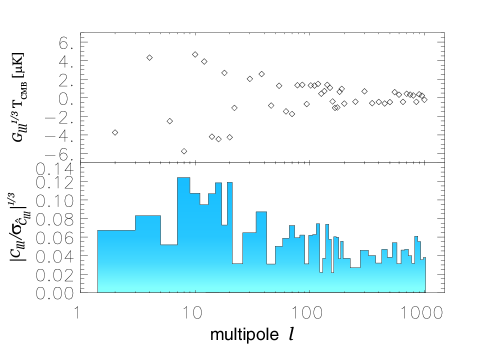
FIG. 1.: The CMB angular bispectrum in the ‘diagonal’ case ($G_{lll}^{1/3}$) from wiggly cosmic strings in a spatially flat model with cosmological parameters $\Omega_{\textrm{CDM}}=0.3$, $\Omega_{\textrm{baryon}}=0.05$, $\Omega_{\Lambda}=0.65$, and Hubble constant $H=0.65{\textrm{km}}{\textrm{s}}^{-1}{\textrm{Mpc}}^{-1}$ [upper panel]. In the lower panel we show the ratio of the signal to theoretical noise $|C_{lll}/\sigma_{\hat{C}_{lll}}|^{1/3}$ for different multipole indices. Normalization follows from fitting the power spectrum to the BOOMERanG and MAXIMA data.

The imprint of cosmic strings on the CMB is a combination of different effects. Prior to the time of recombination strings induce density and velocity fluctuations on the surrounding matter. During the period of last scattering these fluctuations are imprinted on the CMB through the Sachs-Wolfe effect: namely, temperature fluctuations arise because relic photons encounter a gravitational potential with spatially dependent depth. In addition to the Sachs-Wolfe effect, moving long strings drag the surrounding plasma and produce velocity fields that cause temperature anisotropies due to Doppler shifts. While a string segment by itself is a highly non-Gaussian object, fluctuations induced by string segments before recombination are a superposition of effects of many random strings stirring the primordial plasma. These fluctuations are thus expected to be Gaussian as a result of the central limit theorem.

As the universe becomes transparent, strings continue to leave their imprint on the CMB mainly due to the Kaiser-Stebbins effect [24]. This effect results in line discontinuities in the temperature field of photons passing on opposite sides of a moving long string. However, this effect can result in non-Gaussian perturbations only on sufficiently small scales. This is because on scales larger than the characteristic inter-string separation at the time of the radiation-matter equality, the CMB temperature perturbations result from superposition of effects of many strings and are likely to be Gaussian. Avelino et al. [21] applied several non-Gaussian tests to the perturbations seeded by cosmic strings. They found the density field distribution to be close to Gaussian on scales larger than $1.5(\Omega_{M}h^{2})^{-1}$ Mpc, where $\Omega_{M}$ is the fraction of cosmological matter density in baryons and CDM combined. Scales this small correspond to the multipole index of order $l\sim 10^{4}$. We have not attempted a calculation the CMB bispectrum on these scales because the linear approximation is almost guaranteed to fail at such small scales, and because of increased computational cost for higher $l$ multipoles.

In summary, we have developed a numerical method to compute from first principles one of the cleanest non-Gaussian discriminators—the CMB angular bispectrum—in any active model of structure formation, such as cosmic defects, where the energy-momentum tensor is known or can be simulated. Our method does not use CMB sky maps and requires a moderate amount of computations. We applied this method to the computation of some relevant components of the bispectrum produced from a model of cosmic strings and found that the non-zero non-Gaussian signal is unobservable even with forthcoming satellite-based CMB missions. Further computations and improvements using this method will be reported elsewhere.

A Plotting the bispectrum

We explain here our choice for the normalization of the angular bispectrum, as given in Eq. (28). The argument is an extension of the case of the angular power spectrum.

We can express the two-point correlation function at zero lag in terms of the angular spectrum as follows

$$\left\langle\left(\frac{\Delta T}{T}\right)^{2}\right\rangle=\frac{1}{4\pi}\sum_{l}(2l+1)C_{l}.$$ (A1)

In the small angular scale limit, the approximation that $C_{l}$ is a smooth function of the multipole index $l$ is well justified. We can then replace the sum by an integral and get

$$\left\langle\left(\frac{\Delta T}{T}\right)^{2}\right\rangle\approx\frac{1}{4\pi}\int\frac{dl}{l}l(2l+1)C_{l}.$$ (A2)

Now, ${dl/l}=d(\ln(l))$ and therefore $l(2l+1)C_{l}$ is the contribution to the mean squared anisotropy of temperature fluctuations per unit logarithmic interval of $l$. In standard practice, one usually plots $l(l+1)C_{l}/2\pi$ versus $l$, which for large $l$ is proportional to $l(2l+1)C_{l}/4\pi$. On small angular scales, then, this is $\propto l^{2}C_{l}$.

In the case of the three-point correlation function the situation is a bit more involved. Let us consider the skewness:

$$\left\langle\left(\frac{\Delta T}{T}\right)^{3}\right\rangle=\sum_{l_{1}l_{2}l_{3}}\sqrt{\frac{2l_{1}+1}{4\pi}}$$ (A3)

$$\times\sqrt{\frac{2l_{2}+1}{4\pi}}\sqrt{\frac{2l_{3}+1}{4\pi}}\left(\begin{array}[]{ccc}l_{1}&l_{2}&l_{3}\\ 0&0&0\end{array}\right){\mathcal{C}}_{l_{1}l_{2}l_{3}}$$ (A6)

We know that ${\mathcal{C}}_{l_{1}l_{2}l_{3}}$ is smooth in all three indices. We can split the skewness into three sums: the sum of terms where all $l_{i}$ are different, the sum where only two of the three $l_{i}$ are different, and the sum of terms where all $l_{i}$ are equal. Omitting constant factors of $4\pi$, we outline the same procedure as above for the two-point function. For the first sum we get

$$\!\!\int\!\!\frac{dl_{1}}{l_{1}}\!\!\int\!\!\frac{dl_{2}}{l_{2}}\!\!\int\!\!\frac{dl_{3}}{l_{3}} \!\!\!\!l_{1}\sqrt{2l_{1}\!\!+\!\!1}\,\,l_{2}\sqrt{2l_{2}\!\!+\!\!1}\,\,l_{3}\sqrt{2l_{3}\!\!+\!\!1}$$ (A7)

$$\times \left(\begin{array}[]{ccc}l_{1}&l_{2}&l_{3}\\ 0&0&0\end{array}\right)C_{l_{1}l_{2}l_{3}}\,,$$ (A10)

while for the second sum we have

$$\!\!\int\!\!\frac{dl_{1}}{l_{1}}\!\!\int\!\!\frac{dl_{2}}{l_{2}}l_{1}\sqrt{2l_{1}\!\!+\!\!1}\,\,l_{2}\left(2l_{2}\!\!+\!\!1\right)\left(\begin{array}[]{ccc}l_{1}&l_{2}&l_{2}\\ 0&0&0\end{array}\right)C_{l_{1}l_{2}l_{2}}\,,$$ (A13)

and for the third

$$\int\frac{dl}{l}l(2l+1)^{3/2}\left(\begin{array}[]{ccc}l&l&l\\ 0&0&0\end{array}\right)C_{lll}.$$ (A17)

If one is interested in the diagonal terms $C_{lll}$, then, following the last equation, the relevant quantity to plot is given by

$$l(2l+1)^{3/2}\left(\begin{array}[]{ccc}l&l&l\\ 0&0&0\end{array}\right)C_{lll}\,,$$ (A20)

which is $\propto l^{3/2}C_{lll}$ at large $l$.

REFERENCES

- [1] P. de Bernardis, et al, Nature 404, 995 (2000); C.B. Netterfield, et al, preprint astro-ph/0104460.
- [2] A.H. Jaffe, et al, Phys. Rev. Lett. accepted (2001); A.T. Lee, et al, preprint astro-ph/010445.
- [3] N.W. Halverson, et al, preprint astro-ph/0104489.
- [4] J. Magueijo, A. Albrecht, P. Ferreira, D. Coulson, Phys. Rev. D54 (1996) 3727-3744
- [5] A. Gangui, F. Lucchin, S. Matarrese, and S. Mollerach, Astrophys. J. 430, 447 (1994).
- [6] A. Vilenkin and E.P.S. Shellard, “Cosmic Strings and Other Topological Defects”, 2nd Ed., Cambridge, 2000.
- [7] A. Gangui, Science 291, 837 (2001).
- [8] P.P. Avelino and C.J.A.P. Martins, Phys. Rev. Lett. 85, 1370 (2000).
- [9] C. Contaldi, M. Hindmarsh, and J. Magueijo, Phys. Rev. Lett. 82 (1999) 2034; R. Battye and J. Weller, Phys. Rev. D61, 043501 (2000); F.R. Bouchet, P. Peter, A. Riazuelo and M. Sakellariadou, preprint astro-ph/0005022, Phys. Rev. D submitted.
- [10] See e.g. X. Luo, Astrophys. J. 427, L71 (1994); A. F. Heavens, MNRAS 299, 805 (1998); D. Spergel and D. Goldberg, Phys. Rev. D59, 103001 (1999); D. Goldberg and D. Spergel, Phys. Rev. D59, 103002 (1999); J. Magueijo, Astrophys. J. 528, L57 (2000); L. Verde, L. Wang, A. F. Heavens and M. Kamionkowski, preprint astro-ph/9906301; A. Cooray and W. Hu, preprint astro-ph/9910397.
- [11] A. Gangui and J. Martin, MNRAS 313, 323 (2000), preprint astro-ph/9908009.
- [12] U. Seljak and M. Zaldarriaga, Astrophys. J. 469, 437 (1996).
- [13] A. Albrecht, R. Battye, and J. Robinson, Phys. Rev. Lett. 79, 4736 (1997); Phys. Rev. D59, 023508 (1999).
- [14] L. Pogosian and T. Vachaspati, Phys. Rev. D60, 083504 (1999); L. Pogosian, preprint astro-ph/0009307.
- [15] E. Komatsu and D. Spergel, preprint astro-ph/0005036; L. Wang & M. Kamionkowski, Phys. Rev. D61, 063504 (2000).
- [16] A. Gangui and J. Martin, Phys. Rev. D62, 103004 (2000), preprint astro-ph/0001361.
- [17] R. Scaramella and N. Vittorio, Astrophys. J. 375, 439 (1991); M. Srednicki, Astrophys. J. 416, L1 (1993).
- [18] C.J.A.P. Martins and E.P.S. Shellard, Phys. Rev. D54 2535 (1996); preprint hep-ph/0003298.
- [19] N. Turok, U.-L. Pen, and U. Seljak, Phys. Rev. D58, 023506 (1998).
- [20] R. Durrer, A. Gangui and M. Sakellariadou, Phys. Rev. Lett. 76, 579 (1996).
- [21] P.P. Avelino, E.P.S. Shellard, J.H.P. Wu, and B. Allen, Astrophys. J. 507, L101 (1998).
- [22] C.J.A.P. Martins, private communication.
- [23] J.-H.P. Wu et al, preprint astro-ph/9812156.
- [24] N. Kaiser and A. Stebbins, Nature 310, 391 (1984).
- [25] K. Benabed and F. Bernardeau, Phys. Rev. D61, 123510 (2000).
- [26] The numerical code employed here will be made publicly available shortly.