Lensing-induced Non-Gaussian Signatures in the Cosmic Microwave Background

Abstract

We propose a new method for extracting the non-Gaussian signatures on the isotemperature statistics in the cosmic microwave background (CMB) sky, which is induced by the gravitational lensing due to the intervening large-scale structure of the universe. To develop the method, we focus on a specific statistical property of the intrinsic Gaussian CMB field; a field point in the map that has a larger absolute value of the temperature threshold tends to have a larger absolute value of the curvature parameter defined by a trace of second derivative matrix of the temperature field, while the ellipticity parameter similarly defined is uniformly distributed independently of the threshold because of the isotropic nature of the Gaussian field. The weak lensing then causes a stronger distortion effect on the isotemperature contours with higher threshold and especially induces a coherent distribution of the ellipticity parameter correlated with the threshold as a result of the coupling between the CMB curvature parameter and the gravitational tidal shear in the observed map. These characteristic patterns can be statistically picked up by considering three independent characteristic functions, which are obtained from the averages of quadratic combinations of the second derivative fields of CMB over isotemperature contours with each threshold. Consequently, we find that the lensing effect generates non-Gaussian signatures on those functions that have a distinct functional dependence of the threshold. We test the method using numerical simulations of CMB maps and show that the lensing signals can be measured definitely, provided that we use CMB data with sufficiently low noise and high angular resolution.

1 Introduction

Determination of the power spectrum of dark matter fluctuations in the observed hierarchical large-scale structures of the universe remains perhaps the compelling problem in cosmology. Weak gravitational lensing due to the large-scale structure is recognized as a powerful probe of solving this problem as well as of constraining the cosmological parameters (Gunn (1967); Blandford et al. (1991); Miralda-Escude (1991); Kaiser (1992)), because it can fully avoid uncertainties associated with the biasing problem. Recently, several independent groups have reported significant detections of coherent gravitational distortions of distant galactic images (van Waerbeke et al. (2000); Wittman et al. (2000); Bacon, Refregier & Ellis (2000); Kaiser, Wilson & Luppino (2000); Maoli et al. (2000)). On the other hand, the temperature anisotropies in the cosmic microwave background (CMB) can be the most powerful probe of our universe, especially of fundamental cosmological parameters (e.g., Hu, Sugiyama & Silk (1997)). The weak lensing similarly induces distortions in the pattern of the CMB anisotropies, and the lensing signatures will provide a wealth of information on inhomogeneous matter distribution and evolutionary history of dark matter fluctuations between the last scattering surface and present. We then expect that the cosmological implications provided from the measurements of lensing effects on the CMB will be very precise, because there is no ambiguity in theoretical understanding of the primary CMB physics and about the distance of the source plane. However, it is concluded that the weak lensing effects on the CMB angular power spectrum $C_{l}$ is small (e.g. see Seljak (1996) and references therein), although the detailed CMB analyses need to also take into account the lensing contribution. Recently, Seljak & Zaldarriaga (1999) (see also Zaldarriaga & Seljak (1999)) developed a new method for a direct reconstruction of the projected matter power spectrum from the observed CMB map, and showed that it could be successfully achieved if there is no sufficient small scale power of intrinsic CMB anisotropies. In this method, the lensing signals can be extracted by averaging quadratic combinations of the CMB derivative fields over many independent CMB patches like the analysis to extract the distortion effect on distant galactic images, even though the reconstruction maps have a low signal to noise ratio on individual patches.

Excitingly, the high-precision data from the BOOMERanG (de Bernadis et al. (2000); Lange et al. (2000)) and MAXIMA-1 (Hnany et al. (2000); Balbi et al. (2000)) have revealed that the measured angular power spectrum $C_{l}$ is fairly consistent with that predicted by the inflation-motivated adiabatic cold dark matter models (also see Tegmark & Zaldarriaga (2000); Hu et al. (2000)). The standard inflationary scenarios also predict that the primordial fluctuations are homogeneous and isotropic Gaussian (Guth & Pi (1982)), and then statistical properties of any CMB fields can be completely determined from the two-point correlation function $C(\theta)$ or equivalently $C_{l}$ based on the Gaussian random theory (Bardeen et al. (1986) hereafter BBKS; Bond & Efstathiou (1987) hereafter BE). Taking advantage of this predictability, various statistical methods to extract the non-Gaussian signatures induced by the weak lensing have been proposed. Bernardeau (1998) found that the lensing alters a specific shape of the probability distribution function (PDF) of ellipticity parameter for field point or peak for the Gaussian case as a result of an excess of elongated structures in the observed (lensed) map. Although the method could be a powerful probe to measure the matter fluctuations around the characteristic curvature scale of CMB, the beam smearing effect of a telescope is crucial for the detection because it again tends to circularize the deformed structures. Van Waerbeke, Bernardeau & Benabed (2000) then investigated that a statistically correlated alignment between the CMB and distant galactic ellipticities could be detected with a higher signal to noise ratio, provided that a galaxy survey follow-up can be done on a sufficiently large area. We have quantitatively investigated the weak lensing effect on the two-point correlation function of local maxima or minima in the CMB map, and it can potentially probe the lensing signatures on large angular scales such as $\theta\approx 70^{\prime}$ that corresponds to the matter fluctuations with wavelength modes around $\lambda\sim 50h^{-1}{\rm Mpc}$ (Takada, Komatsu & Futamase (2000); Takada & Futamase (2001)). Recently, using numerical simulations, it was shown that the lensing effect causes a change of normalization factors for three morphological descriptions of the CMB map, the so-called Minkowski functionals, against their Gaussian predictions (Schmalzing, Takada & Futamase (2000)).

The purpose of this paper is to develop a new simple method for extracting the lensing-induced non-Gaussian signatures from the CMB map based on the isotemperature statistics. We then focus on specific statistical properties of the intrinsic Gaussian CMB field; a field point that has a larger absolute value of the temperature threshold tends to have a larger absolute value of the curvature parameter defined by a trace of the second derivative matrix of the CMB field, while the ellipticity parameter similarly defined is uniformly distributed independently of the threshold because of the isotropic nature of the Gaussian field. From these features, we expect that the weak lensing causes a larger distortion effect on structures of temperature fluctuations around a point with higher threshold. In particular, the lensing can induce a coherent distribution of the ellipticity parameter correlated with the threshold owing to the coupling between the CMB curvature and the gravitational tidal shear. To extract these characteristic patterns, we define three independent functions based on the isotemperature statistics that are obtained from the averages of quadratic combinations of the second derivatives of CMB field over isotemperature contours with each threshold. As a result, we find the lensing effect on those characteristic functions generates a definite functional dependence of the threshold, and therefore the lensing signals could be easily measured as a non-Gaussian signature since those functions have very specific shapes in the Gaussian (unlensed) case. Using numerical simulations of lensed and unlensed CMB maps including the instrumental effects of beam smearing and detector noise, we investigate the feasibility of the method.

This paper is organized as follows. In §2 we formulate a method for extracting the lensing-induced non-Gaussian signatures using the Gaussian random theory for the primary CMB. In §3 we outline the procedure of numerical experiments of our method using the simulated CMB maps with and without the weak lensing effect. In §4 we present some results in the flat universe with a cosmological constant and investigate the detectability of lensing signatures by taking into account the measurement errors associated with the cosmic variance and the instrumental effects especially for the future satellite mission Planck Surveyor. In the final section some discussions and conclusions are presented.

2 Method: Weak Lensing Effect on Isotemperature Statistics

2.1 Random Gaussian Theory

In this section, we briefly review a relevant part of the Gaussian random theory developed by BBKS and BE for three- and two-dimensional cases, respectively. First, we define the temperature fluctuation field in the CMB map as $\Delta(\mbox{\boldmath$\theta$})\equiv[T(\mbox{\boldmath$\theta$})-T_{\rm CMB}]/T_{\rm CMB}$. Throughout this paper we employ the flat sky approximation developed by BE, and this is a good approximation for our study because the lensing deformation effect on the CMB anisotropies is important only on arcminite scales. The Fourier transformation can be then expressed as $\Delta(\mbox{\boldmath$\theta$})\equiv\int d^{2}\mbox{\boldmath$l$}/(2\pi)^{2}\Delta(\mbox{\boldmath$l$})e^{i\mbox{\boldmath$l$}\cdot\mbox{\boldmath$\theta$}}$, and the statistical properties of the unlensed CMB are completely specified by the angular power spectrum $C_{l}$ defined by $\langle{\Delta(\mbox{\boldmath$l$})\Delta(\mbox{\boldmath$l$}^{\prime})}\rangle=(2\pi)^{2}C_{l}\delta^{2}(\mbox{\boldmath$l$}-\mbox{\boldmath$l$}^{\prime})$.

According to the Gaussian random theory, a certain set of variables $v_{i}(i=1,2,...,N)$ constructed from the CMB field obeys the following joint probability distribution function (PDF);

$$p(\mbox{\boldmath$v$})=\frac{1}{(2\pi)^{N/2}|{\rm det}(M_{ij})|}\exp\left[-\frac{1}{2}v_{i}M^{-1}_{ij}v_{j}\right],$$ (1)

where $M_{ij}$ is the covariance matrix defined by $M_{ij}\equiv\left\langle{(v_{i}-\left\langle{v_{i}}\right\rangle)(v_{j}-\left\langle{v_{j}}\right\rangle)}\right\rangle$, and $M^{-1}$ and ${\rm det}(M_{ij})$ denote the inverse and determinant, respectively. Since we are interested in the lensing distortion effect on the isotemperature contours as a function of the temperature threshold, we pay special attention to statistical properties of the second derivative field of $\Delta$, because the local curvature of CMB is probably a good indicator of the lensing distortion effect as shown latter. It is then convenient to introduce the following variables

$$\nu\equiv\frac{\Delta}{\sigma_{0}},\hskip 20.00003ptX\equiv-\frac{\Delta_{11}+\Delta_{22}}{\sigma_{2}},\hskip 20.00003ptY\equiv\frac{\Delta_{11}-\Delta_{22}}{\sigma_{2}},\hskip 20.00003ptZ\equiv\frac{2\Delta_{12}}{\sigma_{2}},$$ (2)

where $\sigma_{\rm n}$ is defined by $\sigma_{\rm n}^{2}\equiv\int(ldl/2\pi)C_{l}l^{2{\rm n}}$, $\Delta_{ij}\equiv\partial^{2}\Delta/\partial\theta^{i}\partial\theta^{j}$ and $\nu$ is the so-called threshold of temperature fluctuations. To clarify the physical meanings of $X$, $Y$ and $Z$ more explicitly, we express them in terms of two eigenvalues $\lambda_{1}$ and $\lambda_{2}$ for normalized curvature matrix $-\Delta_{ij}/\sigma_{2}$ as

$$X=-(\lambda_{1}+\lambda_{2}),\hskip 20.00003ptY=-2eX\cos(2\varphi),\hskip 20.00003ptZ=-2eX\sin(2\varphi),$$ (3)

where $e$ represents the local ellipticity parameter defined by $e\equiv(\lambda_{1}-\lambda_{2})/[2(\lambda_{1}+\lambda_{2})]$ and $\varphi$ denotes the relative angle between the principal axis of $\Delta_{ij}$ and the $1$-axis. By the meaning of equation above, hereafter we call $X$ a local curvature parameter around a given field point. Moreover, if the isotemperature contour in the neighborhood of local minima or maxima is given by an ellipse of $f(\theta_{1},\theta_{2})=\theta_{1}^{2}/b^{2}+\theta_{2}^{2}/a^{2}$ in the coordinates of principal axes, the parameter $e$ can be expressed in terms of $a$ and $b$ as $e=(a^{2}-b^{2})/[2(a^{2}+b^{2})]$. Hence, $Y$ and $Z$ represent $1$- and $2$-axis components of the local ellipticity parameter of temperature curvature field, respectively. The non-zero second moments of the variables (2) can be then calculated as

$$\left\langle{\nu^{2}}\right\rangle=\left\langle{X^{2}}\right\rangle=2\left\langle{Y^{2}}\right\rangle=2\left\langle{Z^{2}}\right\rangle=1,\hskip 20.00003pt\left\langle{\nu X}\right\rangle=\gamma_{\ast},$$ (4)

where $\gamma_{\ast}=\sigma_{1}^{2}/(\sigma_{0}\sigma_{2})$ (although we will also use the same letter $\gamma$ for a shear component of lensing deformation tensor, we want readers not to confuse $\gamma_{\ast}$ and $\gamma$) and $\gamma_{\ast}$ represents the strength of cross correlation between $X$ and $\nu$ from the relation of $\gamma_{\ast}=\langle{\nu X}\rangle$. Equation (1) tells us that the joint PDF of variables $v_{i}=(\nu,X,Y,Z)$ for one field point becomes

$$p(\nu,X,Y,Z)=\frac{2}{(2\pi)^{2}\sqrt{1-\gamma_{\ast}^{2}}}\exp[-Q],$$ (5)

with

$$2Q\equiv\nu^{2}+\frac{(X-\gamma_{\ast}\nu)^{2}}{(1-\gamma_{\ast}^{2})^{2}}+2Y^{2}+2Z^{2}.$$ (6)

The important result is that $\nu$ and $X$ have the non-vanishing cross correlation, and the term of $\exp[-(X-\gamma_{\ast}\nu)^{2}/(2(1-\gamma_{\ast}^{2}))]$ in equation (5) physically means that structures around a field point with larger absolute threshold tend to have a larger absolute value of the curvature parameter $X$. In fact, this feature is more explicitly clarified by considering the conditional probability distribution for field points with a given threshold $\nu$. Figure 1 shows the distribution of curvature parameter $X$ subject to the constraint that the point has a given threshold $\nu$, where the conditional PDF is defined by $p(X|\nu)\equiv p(\nu,X)/p(\nu)=1/\sqrt{2\pi(1-\gamma_{\ast}^{2})}\exp[-(X-\gamma_{\ast}\nu)^{2}/(2(1-\gamma_{\ast}^{2}))]$. The absence of correlation between $\nu$ and $Y$ or $Z$ is the consequence of the isotropic nature of Gaussian field, more specifically due to the isotropic distribution of an orientation angle of ellipticity parameter.

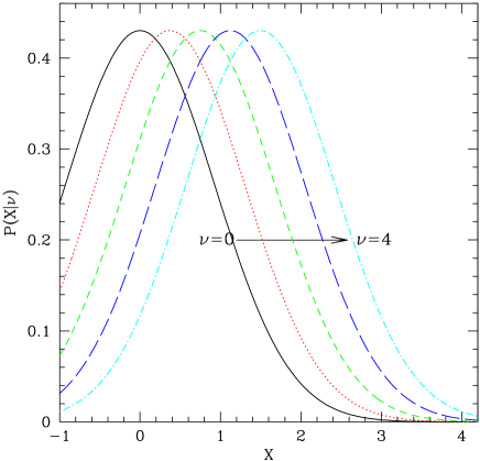
Figure 1: The conditional probability distributions of the curvature parameter $X$ for a field point with the height $\nu=0$ (solid), $\nu=1$ (dot), $\nu=2$ (short dash), $\nu=3$ (long dash), and $\nu=4$ (dot-dash) are plotted for $\gamma_{\ast}=0.35$.

Using the PDF (5), we define the following three independent functions with respect to temperature threshold $\nu_{\rm t}$ that characterize statistical properties of second derivative fields of CMB along isotemperature contours with the threshold $\nu_{\rm t}$;

$$V_{X}(\nu_{\rm t})=\left\langle{\delta(\nu-\nu_{\rm t})X^{2}}\right\rangle=\frac{1}{\sqrt{2\pi}}\exp\left(-\frac{\nu_{\rm t}^{2}}{2}\right)\left[(1-\gamma_{\ast}^{2})+\gamma_{\ast}^{2}\nu_{\rm t}^{2}\right]$$

$$V_{Y}(\nu_{\rm t})=\left\langle{\delta(\nu-\nu_{\rm t})Y^{2}}\right\rangle=\frac{1}{2\sqrt{2\pi}}\exp\left(-\frac{\nu_{\rm t}^{2}}{2}\right)$$

$$V_{Z}(\nu_{\rm t})=\left\langle{\delta(\nu-\nu_{\rm t})Z^{2}}\right\rangle=V_{Y}(\nu_{\rm t}),$$ (7)

where the bracket is defined by $\langle{\cdots}\rangle\equiv\int\!\!d\nu dXdYdZ\cdots p(\nu,X,Y,Z)$ and can be observationally interpreted as average of the considered local quantities performed over all the isocontours in the CMB sky from the assumption of large scale statistical homogeneity. All other averages of quadratic combinations of the second derivatives such as $\left\langle{XY}\right\rangle=\left\langle{XZ}\right\rangle=\left\langle{YZ}\right\rangle$ vanish because of the isotropic nature of the Gaussian field. The functions in equation (7) thus have very specific shapes for the Gaussian case, and we can take advantage of this property in order to extract the non-Gaussian signatures on those functions induced by the lensing distortion effect.

2.2 Lensing distortion effect on the isotemperature contours as a non-Gaussian signature

The CMB photon rays are randomly deflected by the inhomogeneous matter distributions inherent in the intervening large-scale structures of the universe during their propagations from the last scattering surface to us. Therefore, the observed CMB temperature fluctuation field at a certain angular direction $\theta$, $\tilde{\Delta}(\mbox{\boldmath$\theta$})$, is equal to the primary field emitted from the another direction $\mbox{\boldmath$\theta$}+\mbox{\boldmath$\xi$}(\mbox{\boldmath$\theta$})$ on the last scattering surface, $\Delta(\mbox{\boldmath$\theta$}+\mbox{\boldmath$\xi$})$, where $\mbox{\boldmath$\xi$}(\mbox{\boldmath$\theta$})$ is the displacement field. The lensed second derivative field of CMB can be then expressed by

$$\tilde{\Delta}_{ij} = (\delta_{im}+\xi_{m,i})\Delta_{mn}(\delta_{nj}+\xi_{n,j})+\Delta_{m}\xi_{m,ij}$$ (8)

$$= {\cal A}_{im}\Delta_{mn}{\cal A}_{nj}+\Delta_{m}\xi_{m,ij},$$

where ${\cal A}$ is the so-called amplification matrix and $\delta_{ij}$ is the Kronecker delta symbol. Hereafter, the variables with and without tilde symbol denote the lensed and unlensed CMB fields, respectively. The components of ${\cal A}_{ij}$ can be expressed in terms of the local gravitational convergence $\kappa$ and tidal distortion $\gamma$ as

$${\cal A}_{ij}=\left(\begin{array}[]{cc}1-\kappa-\gamma_{1}&-\gamma_{2}\\ -\gamma_{2}&1-\kappa+\gamma_{1}\end{array}\right).$$ (9)

In the weak lensing regime the matrix ${\cal A}$ is always regular, and the variances of $\kappa$, $\gamma_{1}$ and $\gamma_{2}$ are related to each other through

$$\left\langle{\kappa^{2}}\right\rangle=2\left\langle{\gamma_{1}^{2}}\right\rangle=2\left\langle{\gamma_{2}^{2}}\right\rangle=\sigma^{2}_{\kappa}.$$ (10)

We here have not assumed that $\kappa$ and $\gamma_{i}$ are Gaussian, and this is a simple consequence of statistical isotropy of the displacement field. As shown by the several works using the ray tracing simulations through the large-scale structure modeled by N-body simulations, the lensing fields are indeed not Gaussian on angular scales of $\theta\lower 2.15277pt\hbox{$\;\buildrel<\over{\sim}\;$}10^{\prime}$ (Jain, Seljak & White (2000); Hamana, Martel & Futamase (2000)), and we will later discuss the problem how the non-Gaussian features of $\kappa$ could affect our results. The second moment of the convergence, $\sigma_{\kappa}$, is related to the projected matter power spectrum (Kaiser (1992)):

$$\sigma_{\kappa}^{2}=\int\!\!\frac{ldl}{2\pi}P_{\kappa}(l)=\frac{9}{4}H_{0}^{4}\Omega_{m}^{2}\int\!\!\frac{ldl}{2\pi}\int^{\chi_{\rm rec}}_{0}\!\!d\chi a^{-2}(\tau)W^{2}(\chi,\chi_{\rm rec})P_{\delta}\!\left(k=\frac{l}{r(\chi)},\chi\right),$$ (11)

where $P_{\delta}(k)$ and $P_{\kappa}(l)$ denote the three-dimensional power spectrum of matter fluctuations and its projected power spectrum, respectively. $\tau$ is a conformal time, $\chi\equiv\tau_{0}-\tau$, and the subscripts $0$ and “r” denote values at present and the recombination time, respectively. $H_{0}(=100h{\rm km~{}s}^{-1}{\rm~{}Mpc}^{-1})$ and $\Omega_{\rm m0}$ denote the present-day Hubble constant and energy density parameter of matter, respectively. $r(\chi)$ is the corresponding comoving angular diameter distance, defined as $K^{-1/2}\sin K^{1/2}\chi$, $\chi$, $(-K)^{-1/2}\sinh(-K)^{1/2}\chi$ for $K>0$, $K=0$, $K<0$, respectively, where the curvature parameter $K$ is represented as $K=(\Omega_{m0}+\Omega_{\lambda 0}-1)H_{0}^{2}$ and $\Omega_{\lambda 0}$ is the present-day vacuum energy density relative to the critical density. The projection operator $W(\chi,\chi_{\rm rec})$ on the celestial sphere is given by $W(\chi,\chi_{\rm rec})=r(\chi_{\rm rec}-\chi)/r(\chi_{\rm rec})$. As shown later, the effect of the finite beam size $\theta_{\rm fwhm}$ of a telescope on $\sigma_{\kappa}$ appears as a cutoff at $l\lower 2.15277pt\hbox{$\;\buildrel>\over{\sim}\;$}l_{\rm sm}$ in the integration of equation (11) from the relation of $l_{\rm sm}\sim 1/\theta_{\rm fwhm}$ and thus $\sigma_{\rm\kappa}$ also depends on $\theta_{\rm fwhm}$ in a general case. Inversely, by changing the smoothing scale artificially, we could reconstruct the scale dependence of projected matter power spectrum and we will also investigate this possibility. The important result of equation (11) is that the magnitude of $\sigma_{\kappa}$ is sensitive to $\Omega_{m0}$ and particularly to the normalization of matter power spectrum of $P_{\delta}$, which is conventionally expressed in terms of the rms mass fluctuations of a sphere of $8h^{-1}{\rm Mpc}$, i.e., $\sigma_{8}$. Similarly, variances of the second derivative fields of displacement field $\xi_{i}$ can be calculated as

$$\left\langle{\xi_{1,11}^{2}}\right\rangle=5\left\langle{\xi_{1,12}^{2}}\right\rangle=5\left\langle{\xi_{1,11}\xi_{1,22}}\right\rangle=5\left\langle{\xi_{1,12}\xi_{2,22}}\right\rangle=\frac{5}{16}s^{2}$$ (12)

with

$$s^{2}\equiv 4\int\frac{ldl}{2\pi}l^{4}P_{\kappa}(l).$$ (13)

Equation (8) yields the following relations between the lensed (observed) and primary components of the second curvature matrix of temperature fluctuations up to the second order of $\xi$:

$$\tilde{X}=\left[(1-\kappa)^{2}+\gamma^{2}\right]X+2\gamma_{1}Y+2\gamma_{2}Z-\frac{\Delta_{,i}}{\sigma_{2}}\left(\xi_{i,11}+\xi_{i,22}\right),$$

$$\tilde{Y}=\left[(1-\kappa)^{2}+\gamma_{1}^{2}-\gamma_{2}^{2}\right]Y+2\gamma_{1}X+\frac{\Delta_{,i}}{\sigma_{2}}\left(\xi_{i,11}-\xi_{i,22}\right),$$

$$\tilde{Z}=\left[(1-\kappa)^{2}-\gamma_{1}^{2}+\gamma_{2}^{2}\right]Z+2\gamma_{2}X+\frac{\Delta_{,i}}{\sigma_{2}}\xi_{i,12}.$$ (14)

where we have ignored the second order contributions of $\kappa\gamma_{i}$, $\gamma_{1}\gamma_{2}$ and so on because they vanish after the average as a consequence of the statistical isotropy of $\xi_{i}$. Note that the weak lensing does not change the relations between second moments of these lensed variables compared with the Gaussian cases (4); $\langle{\tilde{X}^{2}}\rangle=2\langle{\tilde{Y}^{2}}\rangle=2\langle{\tilde{Z}^{2}}\rangle\approx 1+10\sigma_{\kappa}^{2}$. The equation (14) for $\tilde{Y}$ or $\tilde{Z}$ implies that the lensing effect could induce an ellipticity parameter at a certain field point that arises from a coupling between the curvature parameter $X$ and the gravitational shear $\gamma$ even if the intrinsic ellipticity is zero ($Y=Z=0$). Since this effect is observable only in a statistical sense, we focus our investigations on the problem how the lensing alters statistical properties of the CMB second derivative fields based on the isotemperature statistics.

Now we present theoretical predictions of lensed functions (7) with respect to temperature threshold in the observed CMB map. If we assume that the primary CMB fields on the last scattering surface and the lensing displacement field due to the large-scale structure are statistically independent, after straightforward calculations we can obtain

$$\tilde{V}_{X}(\nu_{\rm t})=\left\langle{\delta(\tilde{\nu}-\nu_{\rm t})\tilde{X}^{2}}\right\rangle=\frac{1}{\sqrt{2\pi}}\exp\left(-\frac{\nu_{\rm t}^{2}}{2}\right)\left[(1+8\sigma_{\kappa}^{2})\left\{(1-\gamma_{\ast}^{2})+\gamma_{\ast}^{2}\nu_{\rm t}^{2}\right\}+2\sigma_{\kappa}^{2}+\frac{\sigma_{1}^{2}}{2\sigma_{2}^{2}}s^{2}\right],$$

$$\tilde{V}_{Y}(\nu_{\rm t})=\left\langle{\delta(\tilde{\nu}-\nu_{\rm t})\tilde{Y}^{2}}\right\rangle=\frac{1}{2\sqrt{2\pi}}\exp\left(-\frac{\nu_{\rm t}^{2}}{2}\right)\left[(1+6\sigma_{\kappa}^{2})+4\sigma_{\kappa}^{2}\left\{(1-\gamma_{\ast}^{2})+\gamma_{\ast}^{2}\nu_{\rm t}^{2}\right\}+\frac{\sigma_{1}^{2}}{4\sigma_{2}^{2}}s^{2}\right],$$

$$\tilde{V}_{Z}(\nu_{\rm t})=\tilde{V}_{Y}(\nu_{\rm t}).$$ (15)

We so far have used the perturbations only for the lensing displacement field $\xi$ and thus these equations (15) are valid for an arbitrary threshold $\nu_{\rm t}$. Equation (15) clearly shows that one of the lensing effects on these functions is the change of their normalization factors. The another important effect is that the lensing generates a characteristic functional dependence of $\nu_{\rm t}$ on $V_{X}(\nu_{\rm t})$, $V_{Y}(\nu_{\rm t})$ and $V_{Z}(\nu_{\rm t})$. This is as a consequence of the coupling between the CMB curvature $X$ and the gravitational tidal shear $\gamma$ through the intrinsic correlation between $\nu_{\rm t}$ and $X$, and physically means that the lensing effect distorts more strongly the isotemperature contours that have larger absolute threshold.

In practice it will be rather difficult to discriminate the change of normalization factors caused by the lensing in equation (15) from the Gaussian case, because measurements of the normalizations in the CMB map might be also sensitive to the systematic errors, for example, due to the discrete effect of pixel in the map. For this reason, we here focus on the non-Gaussian signatures that have a distinct functional dependence of $\nu_{\rm t}$, and consider the following observable functions normalized by their values at $\nu_{\rm t}=0$ as a deviation from the specific function $\exp[-\nu_{\rm t}^{2}/2]$:

$$F_{X}(\nu_{\rm t})\equiv\frac{\tilde{V}_{X}(\nu_{\rm t})}{\tilde{V}_{X}(0)}-\exp\left(-\frac{\nu_{\rm t}^{2}}{2}\right)\approx\exp\left(-\frac{\nu_{\rm t}^{2}}{2}\right)\frac{(1+8\sigma_{\kappa}^{2})\gamma_{\ast}^{2}\nu_{\rm t}^{2}}{1-\gamma_{\ast}^{2}+10\sigma_{\kappa}^{2}-8\sigma_{\kappa}^{2}\gamma^{2}_{\ast}},$$

$$F_{Y}(\nu_{\rm t})\equiv\frac{\tilde{V}_{Y}(\nu_{\rm t})}{\tilde{V}_{Y}(0)}-\exp\left(-\frac{\nu_{\rm t}^{2}}{2}\right)\approx\exp\left(-\frac{\nu_{\rm t}^{2}}{2}\right)\frac{4\sigma_{\kappa}^{2}\gamma_{\ast}^{2}\nu_{\rm t}^{2}}{1+10\sigma_{\kappa}^{2}-4\sigma_{\kappa}^{2}\gamma^{2}_{\ast}},$$

$$F_{Z}(\nu_{\rm t})\equiv\frac{\tilde{V}_{Z}(\nu_{\rm t})}{\tilde{V}_{Z}(0)}-\exp\left(-\frac{\nu_{\rm t}^{2}}{2}\right)=F_{Y}(\nu_{\rm t}),$$ (16)

where we have neglected the terms including contributions of $s^{2}$ in equation (15) because we numerically confirmed that the contributions are always small. In the following discussions, these three independent functions (16) are compared to the results of numerical experiments. Most importantly, equation (16) shows that, although for the Gaussian case in the absence of the lensing we should have $F_{Y}(\nu_{\rm t})=F_{Z}(\nu_{\rm t})=0$ for all $\nu_{\rm t}$ because of $\sigma_{\kappa}=0$, the weak lensing induces distinct non-Gaussian signatures expressed as $\propto\nu_{\rm t}^{2}\gamma_{\ast}^{2}\exp[-\nu_{\rm t}^{2}/2]$. Therefore, those two functions can be direct measures of the lensing distortion effect on the isotemperature contours. The property of $F_{Y}(\nu_{\rm t})=F_{Z}(\nu_{\rm t})$ arises from the statistical random orientations of both the CMB ellipticity parameter and the gravitational tidal shear, and we can use the relation to distinguish or check the lensing signals against other possible secondary non-Gaussian contributions. The lensing effects on $F_{X}$, $F_{Y}$ and $F_{Z}$ depend on two parameters of $\gamma_{\ast}$ and $\sigma_{\kappa}$. Then, note that $\gamma_{\ast}$ is a parameter of the primordial CMB anisotropy field, which is not observable, and is related to the corresponding direct observable quantity $\tilde{\gamma}_{\ast}$ in the lensed CMB map by $\tilde{\gamma}_{\ast}\approx\gamma_{\ast}(1-7\sigma_{\kappa}^{2}/2)$, where $\tilde{\gamma}_{\ast}$ is defined by $\tilde{\gamma}_{\ast}=\tilde{\sigma}_{1}^{2}/(\tilde{\sigma}_{0}\tilde{\sigma}_{2})$ from $\tilde{\sigma}_{0}^{2}=\langle{\tilde{\Delta}^{2}}\rangle$, $\tilde{\sigma}_{1}^{2}=\langle{(\nabla\tilde{\Delta})^{2}}\rangle$ and $\tilde{\sigma}_{2}^{2}=\langle{(\nabla^{2}\tilde{\Delta})^{2}}\rangle$. We will therefore have to treat $\gamma_{\ast}$ as a free parameter in performing the fitting between theoretical predictions (16) and numerical results for the functions $F_{X}(\nu_{\rm t})$, $F_{Y}(\nu_{\rm t})$ and $F_{Z}(\nu_{\rm t})$ in order to determine $\sigma_{\kappa}$. We have then confirmed that $\gamma_{\ast}$ is well constrained mainly by $F_{X}(\nu_{\rm t})$.

2.3 Effect of filtering

We so far have ignored the effects of filtering. Actual CMB temperature maps will be observed with a finite angular resolution, or the artificial filtering method might be used to reduce the detector noise effect (Barreiro et al. (1998)). The measured temperature map is then given by

$$\Delta^{{\cal F}}(\mbox{\boldmath$\theta$};\theta_{s})=\int\!\!d^{2}\mbox{\boldmath$\theta$}^{\prime}W(|\mbox{\boldmath$\theta$}-\mbox{\boldmath$\theta$}^{\prime}|;\theta_{\rm s})\Delta(\mbox{\boldmath$\theta$}^{\prime}),$$ (17)

where $W(\theta;\theta_{\rm s})$ is a window function and throughout this paper we adopt the Gaussian beam approximation expressed by $W(\theta;\theta_{\rm s})=\exp[-\theta^{2}/(2\theta_{\rm s}^{2})]/(2\pi\theta_{\rm s}^{2})$. For the filtering of a telescope, the smoothing angle $\theta_{\rm s}$ can be expressed in terms of its full-width at half-maximum angle $\theta_{\rm fwhm}$ as $\theta_{s}=\theta_{\rm fwhm}/\sqrt{8\ln 2}$. The filtered lensed temperature field is given by

$$\tilde{\Delta}^{{\cal F}}(\mbox{\boldmath$\theta$})=\int\!\!d^{2}\mbox{\boldmath$\theta$}^{\prime}W(|\mbox{\boldmath$\theta$}-\mbox{\boldmath$\theta$}^{\prime}|;\theta_{\rm s})\Delta\left(\mbox{\boldmath$\theta$}^{\prime}+\mbox{\boldmath$\xi$}(\mbox{\boldmath$\theta$}^{\prime})\right).$$ (18)

Similarly, the filtered second derivatives field of the CMB can be expressed as

$$\tilde{\Delta}^{{\cal F}}_{,ij}(\mbox{\boldmath$\theta$}) = \int\!\!d^{2}\mbox{\boldmath$\theta$}^{\prime}W(|\mbox{\boldmath$\theta$}-\mbox{\boldmath$\theta$}^{\prime}|;\theta_{\rm s}){\cal A}_{im}(\mbox{\boldmath$\theta$}^{\prime})\Delta_{,mn}\!\left(\mbox{\boldmath$\theta$}^{\prime}+\mbox{\boldmath$\xi$}(\mbox{\boldmath$\theta$}^{\prime})\right){\cal A}_{nj}(\mbox{\boldmath$\theta$}^{\prime})$$ (19)

$$= \int\!\!d^{2}\mbox{\boldmath$\theta$}^{\prime}W(|\mbox{\boldmath$\theta$}-\mbox{\boldmath$\theta$}^{\prime}|;\theta_{\rm s})\left[\Delta_{,ij}(\mbox{\boldmath$\theta$}^{\prime})+\Delta_{,in}(\mbox{\boldmath$\theta$}^{\prime})\xi_{n,j}(\mbox{\boldmath$\theta$}^{\prime})+\cdots\right]$$

$$= \int\!\!\frac{d^{2}\mbox{\boldmath$l$}}{(2\pi)^{2}}W(\mbox{\boldmath$l$};\theta_{\rm s})\Delta_{ij}(\mbox{\boldmath$l$})e^{i\mbox{\boldmath$l$}\cdot\mbox{\boldmath$\theta$}}+\int\!\!\frac{d^{2}\mbox{\boldmath$l$}}{(2\pi)^{2}}\frac{d^{2}\mbox{\boldmath$l$}^{\prime}}{(2\pi)^{2}}W(|\mbox{\boldmath$l$}+\mbox{\boldmath$l$}^{\prime}|;\theta_{\rm s})\Delta_{in}(\mbox{\boldmath$l$})\xi_{n,j}(\mbox{\boldmath$l$}^{\prime})e^{i(\mbox{\boldmath$l$}+\mbox{\boldmath$l$}^{\prime})\cdot\mbox{\boldmath$\theta$}}+\cdots,$$

where in the first line of right hand side we have used the part integration and assumed that the surface integral is equal to zero for a large CMB survey sky. These equations (18) and (19) mean that the filtering procedure and the lensing effect on the CMB do not commute in a general case. Especially, the last line in the right hand side of equation (19) shows that the information about a certain mode $\mbox{\boldmath$l$}^{\prime}$ of the lensing field $\xi$ is coupled to sidebands of the different $l$ modes of the CMB field. The problem of mode coupling therefore have to be carefully investigated for accurate measurements of our method. However, since the intrinsic CMB anisotropies have a small scale cutoff due to the Silk damping and the directions of the CMB curvature and the lensing deformation field are statistically uncorrelated, we could employ a simple approximation that the filter function $W$ in the equation (19) is applied both to the CMB intrinsic field and the lensing field independently. The variance of convergence field in equations (16) can be then expressed by

$$\sigma^{2}_{\kappa}(\theta_{\rm s})=\int\!\!\frac{d^{2}\mbox{\boldmath$l$}}{(2\pi)^{2}}W^{2}(l;\theta_{\rm s})P_{\kappa}(l),$$ (20)

where $W(l;\theta_{\rm s})=\exp[-l^{2}\theta_{\rm s}^{2}/2]$. Unfortunately, this approximation (20) might not be so accurate since the numerical experiments showed that the magnitude of the convergence field reconstructed by the non-Gaussian signatures in the simulated maps is smaller than the value of $\sigma_{\kappa}$ computed by equation (20). Therefore, the validity or improvement of this approximation should be further investigated using numerical experiments.

3 Models and Numerical Experiments

3.1 Cosmological models

To make quantitative investigations, we consider some specific cosmological models. For this purpose, we adopt the current favored flat universe in the adiabatic cold dark matter model, where the background cosmological parameters are chosen as $\Omega_{\rm m0}=0.3$, $\Omega_{\rm\lambda 0}=0.7$, $h=0.7$, respectively. The flat universe is strongly supported by the recent high precision measurements of $C_{l}$ (de Bernadis et al. (2000); Hnany et al. (2000)). The baryon density is chosen to satisfy $\Omega_{\rm b0}h^{2}=0.019$, which is consistent with values obtained from the measurements of the primeval deuterium abundance (Burles & Tytler (1998)). To compute $C_{l}$ used to make realizations of numerically simulated CMB maps, we used helpful CMBFAST code developed by Seljak & Zaldarriaga (1996). As for the matter power spectrum used to compute lensing contributions to both numerical and theoretical predictions, we employed the Harrison-Zel’dovich spectrum and the BBKS transfer function with the shape parameter from Sugiyama (1995). The free parameter is only the normalization of the present-day matter power spectrum, i.e., $\sigma_{8}$. The nonlinear evolution of the power spectrum is modeled using the fitting formula given by Peacock & Dodds (1996).

3.2 Numerical simulations of CMB map with and without lensing

We perform numerical simulations of the CMB maps with and without the lensing effect following the procedure presented in Takada & Futamase (2001) in detail. First, a realistic temperature map on a fixed square grid can be generated from a given power spectrum, $C_{l}$, based on the Gaussian assumption. Each map is initially $60~{}{\rm deg}^{2}$ area, with a pixel size of about $0.88~{}{\rm arcmin}$ $(=60~{}{\rm deg}/4096)$. A two-dimensional lensing displacement field can be also generated as a realization of a Gaussian process using the power spectrum of convergence field, $P_{\kappa}$, defined by equation (11). Note that we have now employed a technical simplification that the displacement field is assumed to be Gaussian. As explained, the lensing effect is then computed as a mapping between the observed and primordial temperature field expressed by $\tilde{\Delta}(\mbox{\boldmath$\theta$})=\Delta(\mbox{\boldmath$\theta$}+\mbox{\boldmath$\xi$})$. The temperature field on a regular grid in the lensed map is then given by a primordial field on a irregular grid using a simple local linear interpolation of the temperature field in the neighbors (so-called could-in-cell interpolation). In the case of taking into account the instrumental effects of beam smearing and detector noise, we furthermore smooth out the temperature map by convolving the Gaussian window function and then add randomly the noise field into each pixel.

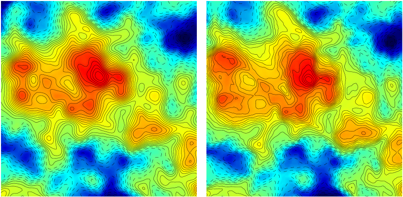
Figure 2: An example of simulated primordial CMB anisotropies map (left) and the lensed map (right). We here adopted the adiabatic CDM flat universe model with $\Omega_{m0}=0.3$, $\Omega_{\lambda 0}=0.7$, and $h=0.7$. The figures are on a side of $2$ degree and the isotemperature contours are drawn in intervals of $\Delta\nu_{\rm t}=0.2$ $(\nu_{\rm t}\equiv\Delta(\mbox{\boldmath$\theta$})/\sigma_{0})$.

Figure 2 shows an example of simulated unlensed (left) and lensed (right) CMB maps, where the isotemperature contours are also drawn in steps of $\Delta\nu_{\rm t}=0.2$. This figure illustrates that the regions around crowded contours with higher absolute temperature threshold and larger curvatures are more strongly deformed by the lensing. Previous works (Seljak & Zaldarriaga (2000); Zaldarriaga (2000)) have pointed out another but partly similar feature that the power of anisotropies on small scales generated by the lensing is correlated with larger scale gradient of the intrinsic CMB field.

3.3 The CMB curvature field

To calculate the second derivative fields of CMB at a certain pixel in the simulated maps, we used a method of finite differences between neighboring pixels around the point:

$$\Delta_{,11}(i,j)=\left[\Delta(i-1,j+1)-2\Delta(i,j)+\Delta(i+1,j)\right]/\delta x^{2},$$

$$\Delta_{,12}(i,j)=\frac{1}{4\delta x^{2}}\left[\Delta(i-1,j-1)-\Delta(i-1,j+1)-\Delta(i+1,j-1)+\Delta(i+1,j+1)\right],$$ (21)

where $\delta x$ is the pixel size and $\Delta(i,j)$ is the local temperature fluctuations at the grid point $(i,j)$.

4 Results and Cosmological Implications

4.1 Numerical results

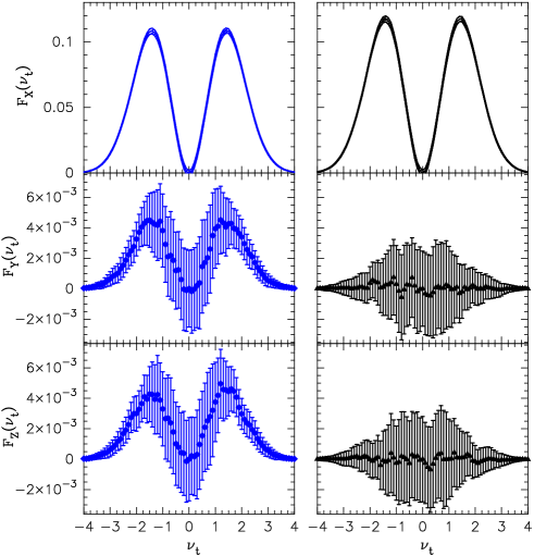
Figure 3: The lensed (left) and unlensed (right) shapes of three functions (16) on the isotemperature statistics with the filter scale of $3$ arcmin and $\sigma_{8}=2.0$ with respect to the temperature threshold $\nu_{\rm t}$, which are computed using the numerical simulations of CMB maps. The background cosmological parameters are $\Omega_{\rm m}=0.3$, $\Omega_{\lambda 0}=0.7$ and $h=0.7$. The triangle and round marks in each panel correspond to the averages obtained from each $150$ independent realizations of the unlensed and lensed maps, respectively. The error bars denote the $1\sigma$ errors due to the cosmic variance computed for $70\%$ sky coverage of the CMB survey. The lensed curves of $F_{Y}(\nu_{\rm t})$ and $F_{Z}(\nu_{\rm t})$ clearly show that the lensing generates a significant functional dependence of $\nu_{\rm t}$ approximately expressed by the from of $\propto\nu_{\rm t}^{2}\exp[-\nu_{\rm t}^{2}/2]$, whereas the unlensed shapes have random errors with both positive and negative values around $F_{Y}(\nu_{\rm t})=F_{Z}(\nu_{\rm t})=0$ in each bin of $\nu_{\rm t}$.

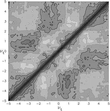
Figure 4: Contours of correlation coefficients, $\langle{(F_{Xi}-\langle{F_{Xi}}\rangle)(F_{Xj}-\langle{F_{Xj}}\rangle)}\rangle/(\sigma_{i}\sigma_{j})$, for estimators of the function $F_{X}(\nu_{\rm t})$ defined by equation (16). Here $F_{Xi}$ and $\sigma_{i}$ denote the values and variance computed from the simulated CMB map in the threshold bin $\nu_{\rm ti}$. The contour is stepped in units of $0.2$ and the solid and dotted contours denote positive and negative values of the coefficients.

In Figure 3, we show the numerical results of the lensed or unlensed three functions (16) with respect to the temperature threshold $\nu_{\rm t}$, which are obtained from each $150$ realizations of CMB maps with $60\times 60~{}{\rm deg}^{2}$ area for the filter scale of $3$ arcmin. All the curves are plotted at intervals of $\Delta\nu_{\rm t}=0.1$. The error bar in each bin corresponds to the cosmic variance associated with the measurements and is estimated by rescaling the variances obtained from all the realizations by a factor $1/8$ when we assume the sky coverage of $70\%$ ($f_{\rm sky}=0.7$) for a survey of the CMB sky. The figure clearly shows that the lensing deformation effect generates a significant functional dependence of $\nu_{\rm t}$ on $F_{Y}(\nu_{\rm t})$ and $F_{Z}(\nu_{\rm t})$ approximately expressed in the form proportional to $\nu_{\rm t}^{2}\exp[-\nu_{\rm t}^{2}/2]$. Especially, the non-Gaussian signatures are pronounced at high absolute threshold such as $|\nu_{\rm t}|\gtrsim 1$ as a result of the strong coupling between the gravitational tidal shear and the large CMB curvature at such high threshold as explained. For a Gaussian case, $F_{Y}(\nu_{\rm t})$ and $F_{Z}(\nu_{\rm t})$ should be equal to zero at all bins of $\nu_{\rm t}$ and thus have both positive and negative large values of the cosmic variance in each bin, although the mean values do not exactly converge to zero yet for the number of our realizations. These results therefore mean that the non-Gaussian signatures induced by the lensing could be significantly distinguished compared to the cosmic variance. In Figure 4 we show the contour map of $\langle{(F_{Xi}-\langle{F_{Xi}}\rangle)(F_{Xj}-\langle{F_{Xj}}\rangle)}\rangle/(\sigma_{i}\sigma_{j})$ calculated from those realizations, where $\langle{F_{Xi}}\rangle$ is the mean value and $\sigma_{i}$ the variance of the estimators of $F_{X}(\nu_{\rm t})$ at threshold bin $\nu_{i}$. We have confirmed that the correlations for $F_{Y}(\nu_{\rm t})$ and $F_{Z}(\nu_{\rm t})$ are similar to the result in this figure. These correlations would be required in order properly to quantify the significance of any departure from Gaussian statistics when performing the fitting between the numerical results and theoretical predictions. Figure 4 indicates and we have actually confirmed that, if we take the data at intervals of $\Delta\nu_{\rm t}\approx 0.5$, the correlation matrix becomes to be very close to diagonal in each bin for all the cases we consider in this paper. Taking into account this result, the following results are shown in intervals of $\Delta\nu_{\rm t}=0.5$.

Figure 5 demonstrates the results with the filtering scale of $5.5$ arcmin computed similarly as in Figure 3. One can see that increasing the filtering scale decreases the magnitude of lensing signals for $F_{Y}(\nu_{\rm t})$ and $F_{Z}(\nu_{\rm t})$, because the filtering again tends to circularize the deformed structures in the CMB map as pointed out by Bernardeau (1998). However, even in this case of $\theta_{\rm fwhm}=5.5^{\prime}$ the lensed curves of $F_{Y}(\nu_{\rm t})$ and $F_{Z}(\nu_{\rm t})$ remain having the distinct functional dependence of $\nu_{\rm t}$ compared to the Gaussian case of $F_{Y}(\nu_{\rm t})=F_{Z}(\nu_{\rm t})=0$. In practice it is important to also take into account the detector noise effect on our method. We here assume the instrumental specification of $217\rm{GHz}$ channel of the satellite mission Planck Surveyor ; the noise level of $\sigma_{N}=4.3\times 10^{-6}$ per a pixel on a side of the FWHM extent ($\theta_{\rm fwhm}=5.5^{\prime}$). The noise field at original fine grid is also convolved with the Gaussian filter of FWHM scale to avoid domination of noise spikes at small angular scales (Barreiro et al. (1998)). Figure 6 shows the results. The noise effect reduces the amplitudes of $F_{X}(\nu_{\rm t})$ compared to that in Figure 5 as a result of the change of quantity $\gamma_{\ast}(\equiv\sigma_{1}^{2}/\sigma_{0}\sigma_{2})$ for the intrisic CMB anisotropies due to the noise. Even in this case, the figure clearly shows that the noise level of Planck does not largely change the lensed shapes of $F_{Y}$ and $F_{Z}$ compared to the results of Figure 5, although the lensing signals at low thresholds such as $|\nu_{\rm t}|\lower 2.15277pt\hbox{$\;\buildrel<\over{\sim}\;$}1.5$ are weakened. Importantly, significant non-Gaussian signatures on $F_{Y}(\nu_{\rm t})$ and $F_{Z}(\nu_{\rm t})$ still remain compared to $F_{Y}(\nu_{\rm t})=F_{Z}(\nu_{\rm t})=0$. This is because our method has so far relied on the normalized observable quantities such as $\nu(\mbox{\boldmath$\theta$})=\Delta(\mbox{\boldmath$\theta$})/\sigma_{0}$ and those quantities are more robust against the systematic contributions of the detector noise than the CMB fields themselves that are certainly affected by the noise. Figure 7 shows the results with $\sigma_{8}=2.5$ similarly as Figure 6. This figure explains that the lensing signals can significantly deviate from the unlensed case if the lensing effect is adequately large.

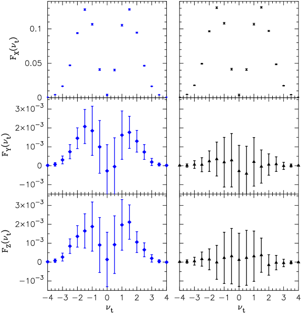
Figure 5: Same as Figure 3 with a 5.5 arcmin filtering scale and $\sigma_{8}=2.0$. All the plots are shown in intervals of $\Delta\nu_{\rm t}=0.5$ taking into account the result of Figure 4.

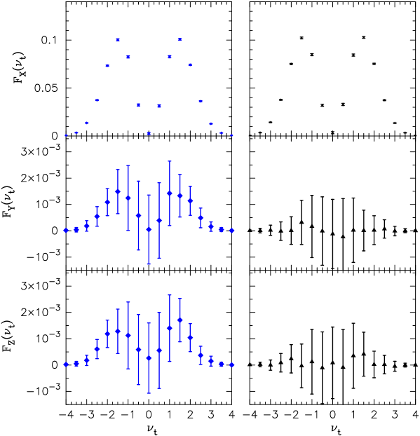
Figure 6: This figure also includes the detector noise effect for the case shown in Figure 5, where we have assumed the noise level of Planck expressed in terms of the variance of noise field per a $5.5$ arcmin FWHM pixel as $\sigma_{\rm pix}=4.3\times 10^{-6}$. Note that the scales of $x$- and $y$- axes are same as in Figure 5.

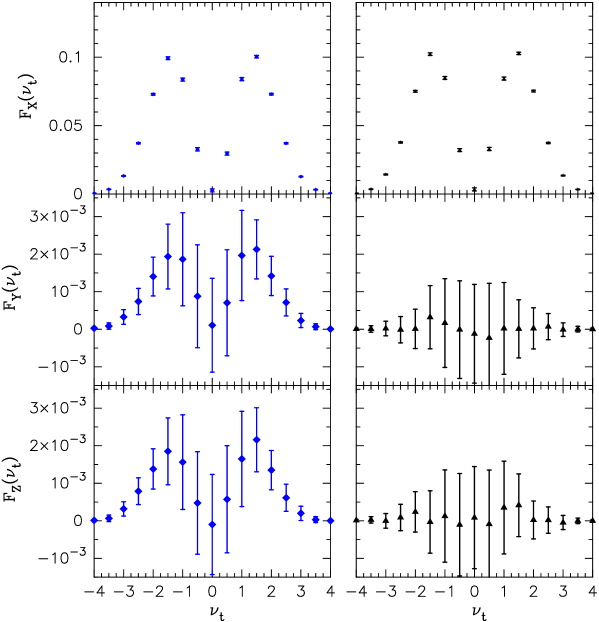
Figure 7: Same as Figure 6 with $\sigma_{8}=2.5$.

4.2 Cosmological implications from the lensing-induced non-Gaussian signatures

Another important question we should address is how useful cosmological information on the large-scale structure formation can be extracted from the lensing signals onto the isotemperature statistics presented in the previous subsection. Since equation (16) shows that the non-Gaussian signatures depend on $\gamma_{\ast}$ and $\sigma_{\kappa}$, we become to consider the problem how accurately the contribution of $\sigma_{\kappa}$ can be determined. As shown by Jain & Seljak (1997), the magnitude of $\sigma_{\kappa}$ is sensitive to $\sigma_{8}$ and $\Omega_{\rm m0}$ parameters for the CDM models and also depends on the filtering scale $\theta_{\rm s}$ for a realistic case. From equation (20) we find that $\sigma_{\kappa}$ thus has following approximate scaling relations for flat universe models around the fiducial model ($\Omega_{\rm m0}=0.3$, $\Omega_{\lambda 0}=0.7$ and $h=0.7$):

$$\sigma_{\kappa}[3^{\prime}]\approx 0.157\times(\theta_{\rm fwhm}/3^{\prime})^{-0.35}\times(\sigma_{8}/2.0)^{1.1}\times(\Omega_{\rm m0}/0.3)^{0.25},$$

$$\sigma_{\kappa}[10^{\prime}]\approx 9.67\times 10^{-2}\times(\theta_{\rm fwhm}/10^{\prime})^{-0.47}\times(\sigma_{8}/2.0)^{1.0}\times(\Omega_{\rm m0}/0.3)^{0.10}.$$ (22)

Furthermore, since more fundamental information is contained in the three-dimensional mass fluctuations, we have to take into account the projection effect (Jain & Seljak (1997); Seljak & Zaldarriaga (1999); Zaldarriaga & Seljak (1999); Takada & Futamase (2001)). The convergence field at $\theta\lower 2.15277pt\hbox{$\;\buildrel<\over{\sim}\;$}10^{\prime}$ depends mainly on the mass fluctuations with wavelength modes of $\lambda\lower 2.15277pt\hbox{$\;\buildrel<\over{\sim}\;$}10h^{-1}{\rm Mpc}$ and the structures distributed in wide redshift ranges of $0\lower 2.15277pt\hbox{$\;\buildrel<\over{\sim}\;$}z\lower 2.15277pt\hbox{$\;\buildrel<\over{\sim}\;$}10$ peaked at $z\approx 3$. The lensing distortion effect on the CMB map can thus be a powerful probe of the large-scale structures up to high redshift in principle, which is not attainable by any other means.

Table 1 summarizes the results obtained for the determination of $\sigma_{\kappa}$ with a best-fit and the $1\sigma$ error, which arises from the cosmic variance or also including errors due to the detector noise effect. The ‘analytic’ value of $\sigma_{\kappa}$ in this table is calculated using the approximation for the beam smearing given by equation (20). We here performed the $\chi^{2}$-fitting between the numerical results and theoretical predictions for $F_{X}(\nu_{\rm t})$, $F_{Y}(\nu_{\rm t})$ and $F_{Z}(\nu_{\rm t})$. Note that we have used each data of the functions in the range of $-4\leq\nu_{\rm t}\leq 4$ at intervals of $\Delta\nu_{\rm t}=0.5$, because the correlation matrix for those data is close to diagonal as explained in Figure 4. Then, the theoretical predictions of $F_{X}(\nu_{\rm t})$, $F_{Y}(\nu_{\rm t})$ and $F_{Z}(\nu_{\rm t})$ are given by two free parameters of $\gamma_{\ast}$ and $\sigma_{\kappa}$ expressed by equation (16). Most importantly, Table 1 clearly shows that $\sigma_{\kappa}$ estimated from the non-Gaussian signatures on $F_{X}$, $F_{Y}$ and $F_{Z}$ could be significantly detected with high signal to noise ratios compared to the unlensed case. Here, $1\sigma$ error for the $\sigma_{\kappa}$ determination corresponds to $\Delta\chi^{2}=2.3$ for the $\chi^{2}$ fitting. Figure 8 demonstrates an example of the best-fit results for the noise case with $\sigma_{8}=2.0$ and $\theta_{\rm fwhm}=5.5$ arcmin. This figure shows that $\sigma_{\kappa}$ is constrained mainly from the numerical data of $F_{Y}(\nu_{\rm t})$ and $F_{Z}(\nu_{\rm t})$ at $|\nu_{\rm t}|\lower 2.15277pt\hbox{$\;\buildrel>\over{\sim}\;$}2$ that have relatively small cosmic variances. On the other hand, $\gamma_{\ast}$ is well constrained only by the data of $F_{X}(\nu_{\rm t})$. Even if we use the value of $\tilde{\gamma}_{\ast}$ directly measured from the lensed simulated CMB maps instead of the fitting parameter $\gamma_{\ast}$ (see the paragraph under equation (16)), it causes only the slight change of results in Table 1. One might then consider a possibility to determine $\sigma_{\kappa}$ by comparing the measured $\tilde{\gamma}_{\ast}$ from the CMB maps to that of $\gamma_{\ast}$ obtained from the fitting of $F_{X}(\nu_{\rm t})$ through the relation of $\tilde{\gamma}_{\ast}=\gamma_{\ast}(1-7\sigma_{\kappa}^{2}/2)$, but the constraint is much weaker than that of using the non-Gaussian signatures on $F_{Y}(\nu_{\rm t})$ and $F_{Z}(\nu_{\rm t})$. Table 1 also shows that the beam smearing effect is crucial for our method and, in the case with $\theta_{\rm fwhm}=8^{\prime}$ and $\sigma_{8}=2.0$ the lensing signatures are obscured by the cosmic variance. On the other hand, the detector noise effect does not largely affect the results. However, we have to note that the best-fit value of $\sigma_{\kappa}$ in all the considered cases is underestimated compared to the analytic value of $\sigma_{\kappa}$ calculated by the approximation (20) for beam smearing effect. The possible reasons for the underestimation are ascribed to the effect of the discrete pixel in the simulated maps or to the mode coupling between the CMB field and lensing field caused by the filtering as explained in §2.3. So far it is concluded based on the following results that the reason is mainly due to the discrete pixel effect. We have confirmed that the best-fit value of $\gamma_{\ast}$ even for the unlensed case by our method also underestimates the value of $\gamma_{\ast}$ calculated by the conventionally used approximation (e.g., Bond & Efstathiou (1987)) expressed in terms of $C_{l}$ and $\theta_{\rm fwhm}$ as $\gamma_{\ast}\equiv\sigma_{1}^{2}(\theta_{\rm fwhm})/\sigma_{0}(\theta_{\rm fwhm})\sigma_{1}(\theta_{\rm fwhm})$, where $\sigma_{\rm i}^{2}(\theta_{\rm fwhm})\equiv\int(ldl/2\pi)l^{2{\rm i}}C_{l}\exp[-l^{2}\theta_{s}^{2}]$ in the context of the small angle approximation and $\theta_{s}=\theta_{\rm fwhm}/\sqrt{8\ln 2}$. For example, values of the best-fit and analytical prediction for $\gamma_{\ast}$ are $0.368$ and $0.38$, respectively, for unlensed case with $\theta_{\rm fwhm}=5.5$ and without the detector noise effect. For the discrete pixel data of simulated CMB maps, it is generally difficult to perform accurate measurements of statistical quantities defined from any derivative fields of CMB compared with their analytical predictions. Schmalzing, Takada & Futamase (2000) have also confirmed that it is crucial for accurate measurements of Minkowski functionals in a realistic CMB map to take into account the effect of discrete pixel, where we have used the interpolation technique. Therefore, we have to further investigate the problem how the $\sigma_{\kappa}$ determination from a realistic CMB map performed by our method can reproduce its simple analytic prediction, for example, by using the numerical simulations combined to the interpolation technique.

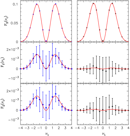
Figure 8: The results of best-fit between the theoretical predictions and the numerical results for the lensed (left: $\sigma_{8}=2.0$) and unlensed (right) cases with $\theta_{\rm fwhm}=5.5$ arcmin and the noise effect. The line in each panel shows the best-fit theoretical prediction (16) (see Table 1).

Table 1: Values of $\sigma_{\kappa}$ from best-fit parameterizations. Errors give the cosmic variance (or also includes the instrumental errors caused by detector noise) for $70\%$ sky coverage survey of the CMB map. Here, the analytic value of $\sigma_{\kappa}$ is calculated by the approximation (20) for the beam smearing effect.

$\sigma_{8}$	filter scale	analytic $\sigma_{\kappa}^{2}\times 10^{2}$	$\sigma_{\kappa}^{2}\times 10^{2}$, best-fit
$0.0$ (no lens)	$3^{\prime}$	-	$0.02\pm 0.03$
$0.0$ (no lens)	$5.5^{\prime}$	-	$0.04\pm 0.03$
$0.0$ (no lens)	$5.5^{\prime}+$noise	-	$0.03\pm 0.04$
$1.5$	$3^{\prime}$	$1.31$	$0.71\pm 0.04$
$1.5$	$5.5^{\prime}$	$0.86$	$0.26\pm 0.03$
$1.5$	$5.5^{\prime}+$noise	$0.86$	$0.23\pm 0.04$
$2.0$	$3^{\prime}$	$2.47$	$1.14\pm 0.04$
$2.0$	$5.5^{\prime}$	$1.57$	$0.42\pm 0.04$
$2.0$	$5.5^{\prime}+$noise	$1.57$	$0.41\pm 0.05$
$2.0$	$8^{\prime}$	$1.15$	$0.07\pm 0.04$
$2.5$	$5.5^{\prime}$	$2.51$	$0.62\pm 0.04$
$2.5$	$5.5^{\prime}+$noise	$2.51$	$0.56\pm 0.05$

5 Discussion and Conclusion

In this paper, we developed a new simple method for extracting the lensing-induced non-Gaussian signatures on the isotemperature statistics in the CMB sky and also investigated the feasibility of the method using the numerical experiments. Importantly, by focusing on the characteristic three independent functions obtained from the averages of quadratic combinations of the second derivatives of CMB field over isotemperature contours with each temperature threshold, it was found that the weak lensing generates non-Gaussian signatures on those functions that have a distinct functional dependence of the threshold. The result is a consequence of the coupling between the gravitational tidal shear and the CMB curvature (defined by $-[\Delta_{,11}+\Delta_{,22}]/\sigma_{2}$) through the intrinsic correlation between the CMB curvature and the temperature threshold predicted by the Gaussian theory. By means of the non-Gaussian signatures, it can be expected that the lensing signals are extracted from an observed CMB data irrespective of the $C_{l}$ measurements or equivalently the assumptions for the fundamental cosmological parameters. Our numerical experiments indeed showed that the method allows us to extract the lensing signals with a high signal to noise ratio, provided that we have CMB maps with sufficiently low noise and high angular resolution as given by the Planck mission. Recently, Seljak & Zaldarriaga (1999) (see also Zaldarriaga & Seljak (1999)) developed a powerful method for a direct reconstruction of the projected power spectrum of matter fluctuations from the lensing deformation effect on the CMB maps. The method focuses on the averages of quadratic combinations of the gradient fields of CMB over a lot of independent patches in the CMB sky like the analysis of the measurements of the coherent gravitational distortion on images of distant galaxies due to the large-scale structure. In the method, the lensing signatures on individual patches are extracted as differences between the measured statistical measures and their all-sky averages. They showed that the reconstruction of input projected matter power spectrum could be successfully achieved if there is no sufficient small scale power of intrinsic CMB anisotropies. In this sense, however, the method partly depends on the statistical measurements of intrinsic CMB anisotropies, and this is main difference between their and our method which we would like to stress. Moreover, our method focuses on the second derivative fields of CMB and, therefore, is more sensitive to the amplitudes of the projected matter power spectrum on smaller angular scales. Anyway, since the lensing signals in the observed CMB sky are weak, we think that some independent statistical methods should be performed to extract them, which could also lead to constraints on the projected matter power spectrum at respective, different angular scales.

Extending our method presented in this paper, one might consider a following possibility to extract the lensing distortion effect. BBKS and BE have shown that structures around local higher maxima or lower minima of temperature fluctuation field tend to have more peaked shape and be more spherically symmetric around the peaks in the Gaussian (unlensed) case. From these features, it can be also expected that the weak lensing causes stronger distortion effect on structures around the higher maxima (or lower minima) and it might provide us more significant non-Gaussian signatures as a function of the temperature threshold of peaks than our method did. However, as quantitatively shown by Bernardeau (1998), the statistical measure for the peaks provides the same or lower signal to noise ratio as or than the statistics for a field point taking into account the cosmic variance, where he investigated the lensing effect on the probability distribution function of ellipticities around field point or peak. This is because the number density of peaks in the CMB sky is not so sufficient for these statistical measurements. For this reason, we prospect a similar conclusion for the signal to noise ratio obtained from the measurements of the lensing distortion effect on the structures around peaks using our method, although this work will have to be further investigated carefully.

Recently, Schamlzing, Takada & Futamase (2000) have shown that the lensing effect on the Minkowski functionals (the morphological descriptions of the CMB map) appears just as a change of their normalization factors against the Gaussian predictions using the numerical experiments. We indeed have confirmed that the analytical predictions for the lensed Minkowski functionals done in the similar way as presented in this paper give the same conclusion as the numerical results. The result comes from the fact that the lensing does not largely change the global topology of the CMB anisotropies in a statistical sense. Likewise, it is known that the gravitational potential from which the shear is generated is invariant under the parity transformation and the lensing does not induce the so-called ‘B-type’ polarization defined from combinations of the derivative fields of CMB fluctuations (Seljak & Zaldarriaga (1999); Zaldarriaga & Seljak (1999)). These results mean that the weak lensing cannot simply generate a new mode of pattern of the CMB anisotropies that is absent in the Gaussian case. For these reasons, in this paper we focus on the another information on statistical properties of the intrinsic CMB that is useful for the study of lensing effect and can be specifically predicted based on the Gaussian random theory. Another issue we should discuss is the possible effect on our results caused by non-Gaussian features on the convergence field of the large-scale structure at $\theta<10^{\prime}$ that are revealed by the ray-tracing simulations (Jain, Seljak & White (2000); Hamana, Martel & Futamase (2000)), which we have ignored in the numerical experiments of the lensed CMB maps. However, since the lensing effect on the CMB can be treated as a mapping, which is expressed as $\tilde{\Delta}(\mbox{\boldmath$\theta$})=\Delta(\mbox{\boldmath$\theta$}+\mbox{\boldmath$\xi$})$, and the lensing contributions to the CMB are always coupled to the contributions from the primary CMB fields, we prospect that the effect will not change the functional dependence of temperature threshold on the lensing-induced non-Gaussian signatures of $F_{X}(\nu_{\rm t})$, $F_{Y}(\nu_{\rm t})$ and $F_{Z}(\nu_{\rm t})$ expressed by equation (16), even if the effect could enhance the magnitudes.

Undoubtedly, other secondary effects could induce non-Gaussian properties in the observed CMB map. The most important effects are the (thermal) Sunyaev-Zel’dovich effect and the foreground contaminations such as Galactic foreground and extragalactic point sources. Those effects can be removed to some extent by using advantages of their spectral properties, although further reliable investigations should be done for any measurements of CMB. Furthermore, in this paper we have presented the lensing-induced non-Gaussian signatures on three independent functions, $F_{X}(\nu_{\rm t}),$ $F_{Y}(\nu_{\rm t})$ and $F_{Z}(\nu_{\rm t})$, and therefore we expect that the property of $F_{Y}(\nu_{\rm t})=F_{Z}(\nu_{\rm t})$ can provide us a clue to resolving the lensing contributions from the other secondary effects.

References

- Bacon, Refregier & Ellis (2000) Bacon, D., Refregier, A., & Ellis, R. 2000, MNRAS, 318, 625
- Bardeen et al. (1986) Bardeen, J. M., Bond., J. R., Kaiser, N., & Szalay, A. S. 1986, ApJ, 304, 15 (BBKS)
- Balbi et al. (2000) Balbi, A. et al. 2000, to appear in ApJ Lett., astro-ph/0005124
- Barreiro et al. (1998) Barreiro, R. B., Sanz, J. L., Martínez-González, & Silk, J. 1998, MNRAS, 296, 693
- de Bernadis et al. (2000) de Bernadis, P. et al. 2000, Nature, 404, 955
- Bernardeau (1998) Bernardeau, F. 1998, A&A, 338, 767
- Blandford et al. (1991) Blandford, R. D., Saust, R. D., Brainerd, A. B., & Villumsen, J. V. 1991, MNRAS, 251, 600
- Bond & Efstathiou (1987) Bond, J. R., & Efstathiou, G. P. 1987, MNRAS, 226, 655 (BE)
- Burles & Tytler (1998) Burles, S. & Tytler, D. 1998 ApJ, 507, 732
- Gunn (1967) Gunn, J. 1967, ApJ, 147, 61
- Guth & Pi (1982) Guth, A. & Pi, S.-Y. 1982, Phys. Rev. Lett., 49, 1110
- Kaiser (1992) Kaiser, N. 1992, ApJ, 388, 272
- Kaiser, Wilson & Luppino (2000) Kaiser, N., Wilson, G., & Luppino, G. 2000, astro-ph/0003338
- Lange et al. (2000) Lange, A. E. et al. 2000, astro-ph/0005004
- Hamana, Martel & Futamase (2000) Hamana, T., Martel, H., & Futamase, T. 2000, ApJ, 529, 56
- Hnany et al. (2000) Hanany, S. et al. 2000, to appear ApJ Lett., astro-ph/0005123
- Hu, Sugiyama & Silk (1997) Hu, W., Sugiyama, N., & Silk, J. 1997, Nature, 386, 37
- Hu (2000) Hu, W. 2000, Nature, 404, 939
- Hu et al. (2000) Hu, W., Fukugita, M., Zaldarriaga, M., & Tegmark, M. 2000, astro-ph/0006463
- Jain & Seljak (1997) Jain, B., & Seljak, U., 1997, ApJ, 484, 560
- Jain, Seljak & White (2000) Jain, B., Seljak, U., & White, S. D. M. 2000, ApJ, 530, 547
- Maoli et al. (2000) Maoli, R., Van Waerbeke, L., Mellier, Y., Schneider, P., Jain, B., Bernardeau, F., Erben, T.,& Fort, B. 2000, astro-ph/0011251
- Miralda-Escude (1991) Miralda-Escude, J. 1991, ApJ, 380, 1
- Schmalzing, Takada & Futamase (2000) Schmalzing, J., Takada, M., & Futamase, T. 2000, ApJ, 544, L83
- Seljak (1996) Seljak, U. 1996, ApJ, 463, 1
- Seljak & Zaldarriaga (1996) Seljak, U., & Zaldarriaga, M. 1996, ApJ, 469, 437
- Seljak & Zaldarriaga (1999) Seljak, U., & Zaldarriaga, M., 1999, Phys. Rev. Lett., 82, 2636
- Seljak & Zaldarriaga (2000) Seljak, U., & Zaldarriaga, M., 2000, ApJ, 538, 57
- Sugiyama (1995) Sugiyama, N. 1995 ApJS, 100, 281
- Takada, Komatsu & Futamase (2000) Takada, M., Komatsu, E., & Futamase, T. 2000, ApJ, 533, L83
- Takada & Futamase (2001) Takada, M. & Futamase, T. 2001, ApJ, 546, 620
- Tegmark & Zaldarriaga (2000) Tegmark, M., & Zaldarriaga, M. 2000, Phys. Rev. Lett., 85, 2240
- van Waerbeke et al. (2000) van Waerbeke, L., Mellier, Y., Erben, T., Cuillandre, J.-C., Bernardeau, F., Maoli, R., Bertin, E., McGracken, H. J., Le Fevre, O., Fort, B., Dantel-Fort Fort, M., Jain, B., & Schneider, P. 2000, A&A, 358, 30
- van Waerbeke, Bernardeau & Benabed (1999) van Waerbeke, L., Bernardeau, F., & Benabed, K. 2000, ApJ, 540, 14
- Wittman et al. (2000) Wittman, D., Tyson, J., Kirkman, D., Dell’Antonio, I., & Bernstein, G. 2000, Nature, 405, 143
- Zaldarriaga (2000) Zaldarriaga, M., 2000, Phys. Rev. D, 62, 063510
- Zaldarriaga & Seljak (1999) Zaldarriaga, M., & Seljak, U. 1999, Phys. Rev. D, 59, 123507