A study of the core of the Shapley Concentration:
VI. Spectral properties of galaxies.

Abstract

We present the results of a study of the spectral properties of galaxies in the central part of the Shapley Concentration, covering an extremely wide range of densities, from the rich cluster cores to the underlying supercluster environment.
Our sample is homogeneous, in a well defined magnitude range ($17\leq b_{J}\leq 18.8$) and contains $\sim 1300$ spectra of galaxies at the same distance, covering an area of $\sim 26$ deg². These characteristics allowed an accurate spectral classification, that we performed using a Principal Components Analysis technique.
This spectral classification, together with the [OII] equivalent widths and the star formation rates, has been used to study the properties of galaxies at different densities: cluster, intercluster (i.e. galaxies in the supercluster but outside clusters) and field environment.
No significant differences are present between samples at low density regimes (i.e. intercluster and field galaxies). Cluster galaxies, instead, not only have values significantly different from the field ones, but also show a dependence on the local density.
Moreover, a well defined morphology-density relation is present in the cluster complexes, although these structures are known to be involved in major merging events. Also the mean equivalent width of [OII] shows a trend with the local environment, decreasing at increasing densities, even if it is probably induced by the morphology-density relation.
Finally we analyzed the mean star formation rate as a function of the density, finding again a decreasing trend (at $\sim 3\sigma$ significance level). Our analysis is consistent with the claim of Balogh et al. (1998) that the star formation in clusters is depressed.

1 Introduction

Since the discovery that galaxies in clusters are different from those in the field (Hubble & Humason 1931), it has been recognized that the environment must play an important role in determining the characteristics of the galaxy population. In fact, at present the existence of a morphology-density relation, spanning a large range of densities from rich clusters (Dressler 1980) to groups (Postman & Geller 1984), is generally accepted.

More intriguing is to determine whether the star formation is influenced by the environment or the different galaxy population in clusters is merely a consequence of the morphology-density relation, and which mechanism is responsible for the change of the morphological mix.

From the observational point of view, other indications of differences between field and cluster galaxies come from the Butcher-Oemler effect (i.e. the bluening of cluster galaxies as a function of redshift; Butcher & Oemler 1984) and from the observation of “anaemic” or “HI deficient” spirals (i.e. with reduced content of HI with respect to field galaxies of the same morphological type; Bothun 1982) in local clusters.
Very recently, analysing the CNOC1 cluster sample in the redshift range $0.2-0.5$, Balogh et al. (1998) found that the cluster environment not only affects the morphological mix but also suppresses the star formation.
Various physical mechanisms (as for example galaxy harassment, tidal stripping, ram pressure) have been proposed to explain the differences between field and cluster galaxies: however, the influence of these phenomena on the changes in star formation rate remains still uncertain.

In this context, an interesting point is that to compare properties of field galaxies with those of galaxies which reside in rich superclusters, but outside clusters.
In fact, considering that up to scales of 2  h^-1 Mpc superclusters as the Great Wall are dominated by galaxy groups (Ramella, Geller & Huchra 1992), a morphology-density relation may exist also in these lower density environments, leading to a difference in the morphological mix between field and supercluster galaxies. On the other hand, Hoffman, Lewis & Salpeter (1995) found that the luminosity function of late type objects in the Great Wall does not differ from that of field galaxies.

The aim of the present paper is to investigate the morphology-density relation in a wide range of densities, using an homogeneous sample of $\sim 1300$ spectra of galaxies in different environments, like rich cluster cores, supercluster, field. Our sample cover the central region of the Shapley Concentration, which has an average density excess in galaxies of $\displaystyle{{N}\over\bar{N}}=11.3\pm 0.4$ on a scale of $\sim 10$  h^-1 Mpc (Bardelli et al. 2000). This region is dynamically very active and is characterized by the presence of two high density complexes formed by merging clusters (Bardelli et al. 1994, 1998a, 1998b, 2001). These complexes are embedded in a planar structure of $\displaystyle{{N}\over\bar{N}}\sim 4$, which resembles the Great Wall and represents the supercluster environment. Finally, a subsample of galaxies from the ESP survey (Vettolani et al. 1997) is used to derive the reference values for the “true” field environment $\displaystyle({{N}\over\bar{N}}\sim 1)$.

The paper is organized as follows. In Sect. 2 we present our classification technique, based on the Principal Components Analysis, in Sect. 3 we describe our data and in Sect. 4 we show the results of the spectral classification. In Sect. 5 we analyze the relations between the spectral morphology and the local environment and in Sect. 6 we present the results about the emission line properties and the star formation rates. Finally, the results are discussed and summarized in Sect. 7.

2 Spectral classification

Morphological classification of galaxies from optical images (Hubble 1936; de Vaucouleurs & de Vaucouleurs 1961; Sandage 1975) is generally performed analysing the luminosity profile of a galaxy. This method requires a very careful study of the images which implies a parametric fit of the luminosity profile: in fact it is necessary to fit the luminosity profile of a galaxy to distinguish between a bulge and an exponential disk. Moreover a galaxy may have a different appearance if observed using different filters or at different redshifts (O’Connell & Marcum 1997).
Even the advent of the Hubble Space Telescope does not prevent every existing method of morphological classification to be strongly dependent on the image resolution, on the adopted filters and on the redshift of the galaxy.

An alternative approach to the morphological classification can be made if we consider the spectral energy distribution (SED), which resumes the main physical features of a galaxy. In fact, for a given galaxy, the SED measures the relative contribution of the various stellar populations and gives constraints to the amount of gas and to the mean metallicity.
The spectral energy distribution is then useful to classify the galaxies in a spectral sequence rather than in a morphological one. Generally, a galaxy is formed by three main components: gas, young stars and old stars. These components contribute to outline both the main morphological features (bulge, spiral arms, etc.) and the spectral ones (continuum shape, absorption and emission lines). Moreover, dealing with big amounts of data, spectra are easier to handle than bidimensional images, allowing an automatized classification of galaxies.
In the past decade, such an automatization has been attempted by many authors. The most used technique, applied to surveys of galaxy spectra, is the Principal Components Analysis (hereafter PCA, Connolly et al. 1995; Folkes, Lahav & Maddox 1996; Sodré & Cuevas 1997; Galaz & de Lapparent 1998; Sodré, Cuevas & Capelato 1998; de Theije & Katgert 1999). Using this technique, although with different approaches, these authors found that the whole distribution of spectral types can be described by only two parameters.
Zaritsky, Zabludoff & Willick (1995) assumed instead the a priori hypothesis that each spectrum can be represented as a linear combination of three components: one representing old stellar populations (typical K star spectrum), one representing young stellar populations (typical A star spectrum) and an emission lines component. Anyhow this approach has given results very similar to those obtained with the application of PCA.

Figure 1: Isodensity contours of the bidimensional distribution of the galaxies in the $b_{J}$ magnitude bin $17-19.5$ in the UKSTJ plates which cover the central part of the Shapley Concentration. The data have been binned in $2$ $\times$ $2$ arcmin pixels and then smoothed with a Gaussian with a FWHM of $6$ arcmin. For the Abell clusters present in the plates, circles of one Abell radius have been drawn (dashed curves). Solid circles represent the MEFOS fields.
a) Plate 509; b) Plate 444; c) Plate 443. The two most evident systems are the A3558 (plate 444) and the A3528 (plate 443) cluster complexes. The relative positions of the fields is shown in the upper right panel, where small circles represent OPTOPUS observations on the cluster complexes (which for clearness were not drawn on the isodensity contours).

2.1 The PCA technique

The method we have chosen to perform the spectral classification of our galaxy sample is the Principal Components Analysis. An exhaustive description of the PCA technique can be found in Murtagh & Heck (1987) or in Kendall (1980): here we underline only its main features of interest for our work.
The PCA applies to a sample of $N$ objects (in our case $N$ spectra) which can be described by $M$ coordinates (in our case, for each spectrum, the fluxes of single pixels). In this $M$-dimensional hyperspace, each object is represented by a point and the sample is a cloud of points. The main idea of the PCA is to find an orthonormal base of eigenvectors (of dimension $P<\min[N,M]$) whose linear combination represents the sample. The eigenvectors are found by minimizing the euclidean distance of the points from the new base: these new axes are called Principal Components (PCs). The eigenvalues give the variance of each PC. An higher value of the variance indicates a lower distance between the cloud of points and the new axis relative to the eigenvalue, then a better description of the sample.
Each spectrum S is normalized by its norm as:

$${\bf S}^{norm}=\frac{\bf S}{\sqrt{\sum_{j=1}^{M}{\bf S}_{j}^{2}}}$$ (1)

Other methods of normalization can be used (for instance a flux normalization at a given wavelength), but Connolly et al. (1995) have demonstrated that the various methods of normalization do not have relevant effects onto the PCA results.
The techniques generally used to reduce the input matrix are three: the sum of squares and cross product matrix method (SSCP), the variance-covariance matrix method (VC) and the correlation matrix method (C). The first method (SSCP) does not apply any rescaling on the data nor centre the cloud of points. The normalized spectra then lie on the surface of an $M$-dimensional hypersphere of radius 1, and the first PC has the same direction of the average spectrum. The second method (VC) places instead the new origin onto the centroid of the sample. The latter method (C) centres the cloud of points and rescales the data in such a way that the distance between variables is directly proportional to the correlation between them.
It is worth to stress that neither the PCs nor the projections on them obtained with the three different methods are the same. However, if the cloud of points is concentrated in a small portion of the hypersphere of radius 1, then the first PC obtained with VC method will have almost the same direction of the second PC obtained from SSCP method (Galaz & de Lapparent 1998).
After performing the PCA, it becomes possible to reconstruct each spectrum S^norm as:

$${\bf S}_{approx}=\sum_{k=1}^{N_{PC}}\alpha_{k}{\bf E}_{k}$$ (2)

where S_approx is the S^norm spectrum reconstructed using only the first $N_{PC}$ PCs and $\alpha_{k}$ is the projection of S^norm onto the eigenspectrum (principal component) E_k.

2.2 Application of the PCA to the data

The three methods described in the previous section have been tested on our dataset. We decided to use the SSCP method for the following reasons. First, the first three PCs are sufficient to reconstruct $\sim$99% in flux of the sample, i.e. at the same percentage of reconstructed flux, a lower number of components is enough. As a comparison, the VC method gives a percentage of $\sim$87% and the C method gives a percentage less than 80% for the first three principal components. Moreover, plotting $\alpha_{1}$ vs. $\alpha_{2}$, which are the projections onto the first two PCs, the diagram has a smaller scatter, indicating a better definition of a spectral sequence (see below). Finally, the first three principal components have a straightforward physical interpretation, although this is not an objective criterion for choosing a method.
Using the SSCP method it is then possible to perform a spectral classification dependent only on three parameters. Moreover, following Galaz & de Lapparent (1998), we can apply a change of coordinates, from ($\alpha_{1}$, $\alpha_{2}$, $\alpha_{3}$), the projections onto the PCs, to ($r$, $\delta$, $\theta$), the radius, the azimuth and the polar angle measured from the equator, respectively:

$$\alpha_{1} = {\it r}\cos\theta\cos\delta$$ (3)

$$\alpha_{2} = {\it r}\cos\theta\sin\delta$$ (4)

$$\alpha_{3} = {\it r}\sin\theta$$ (5)

It is then possible to isolate the values of $\delta$ and $\theta$ from $r$ (which is equal to 1, because of the applied normalization):

$$\delta = \arctan\left(\frac{\alpha_{2}}{\alpha_{1}}\right)$$ (6)

$$\theta = \arctan\left\{\left(\frac{\alpha_{3}}{\alpha_{2}}\right)\sin\left[\arctan\left(\frac{\alpha_{2}}{\alpha_{1}}\right)\right]\right\}$$ (7)

The parameters used to perform the spectral classification are then reduced to only two: we have in fact eliminated the magnitude parameter (represented by $r$) having performed a normalization of the spectra. In general, morphological types do depend on the magnitude, because of the differences in luminosity functions of galaxies going from ellipticals to irregulars (see f.i. Binggeli, Sandage & Tammann 1988); however, as described below, we have a very small range in magnitudes that allows us to neglect this parameter.
Moreover it is possible to associate a physical meaning to $\delta$ and $\theta$. In fact, $\delta$ represents the contribution of the blue over the red part of the spectrum, i.e. of the young stellar population relative to the older one, while $\theta$ represents the importance of emission lines in a galaxy spectrum and could then be an indicator of star formation (see below).

Table 1: Number of objects in the various samples.

	$N_{tot}$	$N_{z}$	$N_{Shapley}$	$N_{spectra}$
A3528 complex $(17\leq b_{J}\leq 18.8)$	674	504	402	350
A3558 complex $(17\leq b_{J}\leq 18.8)$	722	464	421	264
Intercluster sample $(17\leq b_{J}\leq 18.8)$	1839	459	166	161
A3528 complex $(b_{J}\leq 19.5)$	1439	678	527	447
A3558 complex $(b_{J}\leq 19.5)$	1582	727	633	397

3 The data

The photometric data catalogue is the COSMOS/UKST galaxy catalogue of the southern sky (Yentis et al. 1992) obtained from automated scans of UKST $J$ plates by the COSMOS machine.
Spectroscopic observations were obtained using the ESO 3.6-m telescope in La Silla equipped with the OPTOPUS multifibre spectrograph (Lund 1986), for observations in the regions of cluster complexes, and with the MEFOS multifibre spectrograph (Bellenger et al. 1991; Felenbok et al. 1997) for observations in the intercluster region. In Figure 1 we show the position of the observed OPTOPUS and MEFOS fields, superimposed on the galaxy isodensity contours.
A further spectral sample from the ESO Slice Project (ESP) galaxy redshift survey (Vettolani et al. 1997) has been considered in order to have a comparison of supercluster spectra with those of “true” field galaxies.
From all these samples, we have considered only galaxies in the velocity range $10000-22500$ km/s, in order to limit the spectral analysis to the physical extension of the Shapley Concentration (Bardelli et al. 2000). Moreover, given the fact that the intercluster survey is limited to the magnitude range 17 $\leq$ $b_{J}$ $\leq$ 18.8, when we compare the cluster galaxy properties with the intercluster ones, we use subsamples with these magnitude limits. This choice avoids possible biases deriving from sampling of luminosity functions of various morphological types at different magnitudes. On the contrary, when we consider only properties of cluster galaxies, we use the samples in the whole magnitude range ($b_{J}\leq 19.5$).

In Table 1 the relevant numbers for each sample are given. In column (1) we give the sample name, in column (2) the number of COSMOS/UKST galaxies inside the survey area and in column (3) the number of galaxies with redshift (including literature measurements). Column (4) reports the number of objects belonging to the Shapley Concentration: among these, we could classify only objects with spectra observed by us. This number is reported in column (5).

3.1 The A3528 complex

The region considered to sample the A3528 complex is part of the UKST $J$ plate 443 and has a dimension on the plane of the sky of $\alpha\times\delta\sim 2\aas@@fstack{\circ}7\times 3\aas@@fstack{\circ}8$, in the range $12^{h}51^{m}<\alpha(2000)<13^{h}15^{m}$ and $-31^{o}36\arcmin<\delta(2000)<-28^{o}00\arcmin$ (Bardelli, Zucca & Baldi 2001).
The spectroscopic observations were performed with the OPTOPUS multifibre spectrograph; we used the ESO grating $\#\ 15$ allowing a resolution of $\sim 12$ Å in the wavelength range $3700-6024$ Å. The detectors were Tektronic $512\times 512$ CB CCDs (ESO $\#16$ for 1991 run; ESO $\#32$ for 1993 run) with a pixel size of $4.5$ Å. Detector $\#32$ has a particularly good responsive quantum function in the blue ($\sim 70\%$ at $4000$ Å), if compared with detector $\#16$.
All the details on the reduction steps can be found in Bardelli et al. (1994): however, it could be important to stress that we normalized the fiber transmission rescaling the spectra in order to have the same continuum–subtracted flux of the sky emission line [OI]$\lambda$5577.

3.2 The A3558 complex

The region considered to sample the A3558 complex lies on the UKST $J$ plate 444 and has a dimension on the plane of the sky of $\alpha\times\delta\sim 3\aas@@fstack{\circ}2\times 1\aas@@fstack{\circ}4$, in the range $13^{h}22^{m}06^{s}<\alpha(2000)<13^{h}37^{m}15^{s}$ and $-32^{o}22\arcmin 40\arcsec<\delta(2000)<-30^{o}59\arcmin 30\arcsec$ (Bardelli et al. 1994, Bardelli et al. 1998a).
The spectroscopic observations were performed with the same instruments and the setup used for the A3528 complex survey (see above). It is worth noting from Table 1 that the number of spectra available for the classification in this sample is lower than in the sample relative to the A3528 complex: this is due to the large number of galaxies with a redshift determination in the literature for the A3558 complex and then not re-observed in our survey.

3.3 The intercluster sample

The intercluster survey, described and analyzed in detail in Bardelli et al. (2000), has been performed in order to study the distribution of galaxies in the Shapley Concentration outside the clusters. The spectroscopic observations covered part of the UKST $J$ plates 443, 444 and 509 and were obtained with the MEFOS spectrograph. In order to maximize the performances of this instrument, we adopted the magnitude range $17-18.8$.
The spectra, obtained with the CCD TEK512 CB # 32 and the ESO grating $\#15$, have a resolution of $\sim 12$ Å and a pixel size of $\sim 4.6$ Å: data were reduced and cross-correlated in the same way as done for the cluster complexes.

3.4 The ESP sample

The ESP galaxy redshift survey (Vettolani et al. 1997) extends over a strip of $\alpha\times\delta$=$22^{\circ}\times 1^{\circ}$, plus a nearby area of $5^{\circ}\times 1^{\circ}$, five degrees west of the main strip, in the South Galactic Pole region. The whole ESP sample, together with the detailed description of the survey, is available in Vettolani et al. (1998).
To our aims it is sufficient to remember that the spectroscopic observations were performed at the ESO 3.6-m telescope in La Silla, using the multifibre spectrographs OPTOPUS and MEFOS with the same instrumental setup used for our surveys on the Shapley Concentration. However, given the fact that the wavelength coverage of some ESP spectra is limited to 3900 - 6100Å, in order to include the [OII]$\lambda$3727 line in all the rest frame spectra we are forced to use only galaxies with $v>15800$ km/s, instead $v>10000$ km/s as done for all the other samples. Applying also the $17-18.8$ magnitude cut, we obtained a sample of $\sim 300$ galaxies. The mean galaxy density in this sample is consistent with that of the whole ESP survey.
The ESP galaxies are supposed to be “true” field galaxies and should represent a well defined reference sample to analyse the variations in morphological mixing inside the Shapley supercluster.

Figure 2: The first three principal components (PCs) obtained by PCA. The main spectral lines of each PC are represented.

Table 2: Galaxies of Kennicutt’s sample.

name	type	name	type
NGC 3379	E0	NGC 3147	Sb
NGC 4472 (1)	E1/S0	NGC 3227 (3,4)	Sb
NGC 4648	E3	NGC 3627	Sb
NGC 4889 (2)	E4	NGC 5248	Sbc
NGC 3245	S0	NGC 6217	SBbc
NGC 3941	SB0/a	NGC 2276 (3)	Sc
NGC 4262 (1)	SB0	NGC 2903	Sc
NGC 5866	S0	NGC 4631	Sc
NGC 1357	Sa	NGC 4775	Sc
NGC 2775	Sa	NGC 6181	Sc
NGC 3368	Sab	NGC 6643	Sc
NGC 3623	Sa	NGC 4449	Sm/Im
NGC 1832	SBb	NGC 4485 (3)	Sm/Im

(1) Virgo cluster member; (2) Coma cluster member; (3) strongly interacting or merging galaxy; (4) galaxy with a Seyfert 2 nucleus.

3.5 Preparing the data for the PCA algorithm

The spectral sample described in previous sections has been prepared for the application of the PCA via the SSCP method. The spectra have been de-redshifted to the rest frame, reduced at the same rest frame dispersion (4.5 Å/pix) and cut in the same wavelength range (3705 - 5500 Å). This wavelength band has been chosen in order to observe all the spectral features between the [OII] $\lambda$3727 emission line and the Ca+Fe $\lambda$5269 absorption line. The number of pixels (i.e. the number of coordinates describing each spectrum in the PCA) is 400.
In order to have a link between our PCA spectral classification and the classical morphologies of galaxies, we added to our sample a set of spectra of nearby galaxies from the spectrophotometric atlas of Kennicutt (1992a): these spectra are of good quality and refer to galaxies with known morphology. From the original atlas, we used the 26 normal galaxies listed in Table 2. These spectra have been reduced to the same wavelength range and dispersion of our sample: indeed, it is necessary to run the PCA procedure at the same time for all the spectra (our data plus Kennicutt’s data) in order to obtain a relative scale to define the spectral sequence.

4 Results from the PCA

The PCA classification has been applied to the sample of spectra from the cluster complexes, the intercluster field, the ESP survey subsample and the Kennicutt’s atlas, in the magnitude range $17\leq b_{J}\leq 18.8$. In order to make a relative comparison between the morphological mix of the two cluster complexes, we ran the PCA also in the whole magnitude range ($b_{J}\leq 19.5$) for these samples, finding similar results.
The first three principal components are represented in Figure 2. The first principal component (PC1) contributes to 96.7% in flux of the sample and is characterized by a prominent red continuum relative to the blue one. It shows spectral features like a clear 4000Å break, a number of absorption lines like the pair K $\lambda$3934 and H $\lambda$3969, H$\delta$ $\lambda$4102, G $\lambda$4304 and MgI $\lambda$5175, and the forbidden emission line of [OII] $\lambda$3727. The continuum of this spectrum resembles closely that of an early-type galaxy like an E or an S0: however, the presence of the [OII] emission line indicates that this PC has also some characteristics of early spirals, like Sa and Sb. The contribution of PC1 is dominant because our sample is mainly composed by early-type galaxies.
The second principal component (PC2) contributes on average to 2.0% in flux of the sample. The blue part of the spectrum is enhanced with respect to the red one and the [OII] emission line is clearly more prominent than in PC1; moreover, the emission features of H$\beta$ $\lambda$4861 and of [OIII] $\lambda\lambda$4959,5007 clearly appear. This eigenspectrum is characterized by less important absorption features and resembles the spectrum of a galaxy with star formation activity, where the dominant population is constituted by the blue young stars, which dominates the continuum. The ongoing star formation activity in such a type of galaxy can be detected by the presence of nebular emission lines too.
The third principal component (PC3) contributes on average to 0.3% in flux of the spectral sample. Its continuum is almost flat and dominated by the emission lines, stronger than in PC2, of [OII], H$\beta$ and [OIII]: it presents also the H$\gamma$ $\lambda$4341 emission line, although not so prominent like the others, which is not present in PC2. Hence this eigenspectrum represents essentially the emission features in a galaxy spectrum, which can be related, expecially in the case of [OII], to the presence of an ongoing star formation activity (Kennicutt 1992b).
The other principal components contribute marginally to the flux of our spectral sample (0.12% for the fourth, 0.07% for the fifth, etc.) and have not a straightforward physical interpretation. Therefore we have decided to neglect them and to perform the spectral classification using only the first three eigenspectra, which contribute together to $\sim$99% in flux of the sample.
Then, as described in Sect. 2.2, we applied a change of coordinates from ($\alpha_{1}$, $\alpha_{2}$, $\alpha_{3}$) to ($\delta$, $\theta$): the $\delta$-$\theta$ plot is shown in Figure 3, for all the spectra of the sample in the Shapley Concentration. The Kennicutt’s galaxies are plotted with big points and with different symbols for each Hubble type. To simplify the figure, we have decided to put barred and normal spirals (like Sa and SBa) in the same category and intermediate types have been put in the earliest category (for instance, an Sab galaxy has been marked as Sa). The two galaxies labelled Ir (irregulars) are Sm/Im.

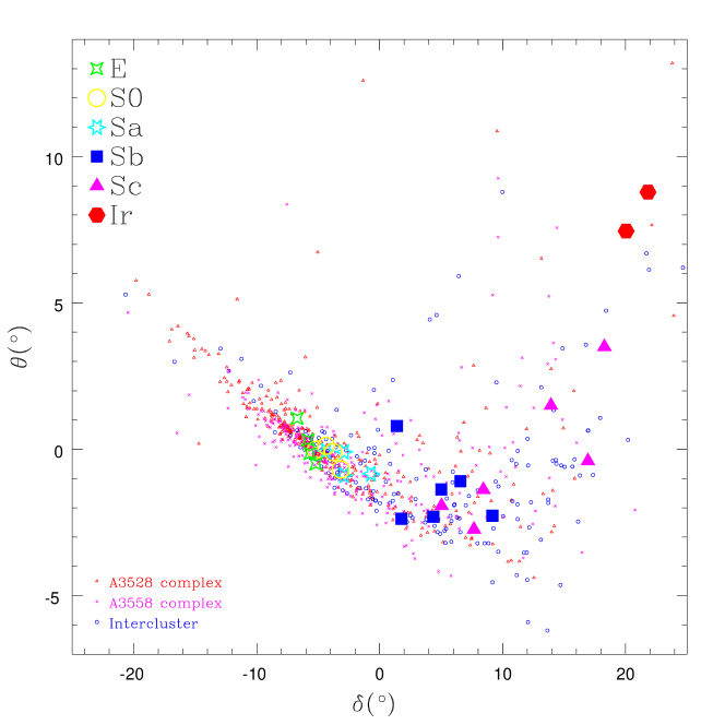
Figure 3: The classification diagram $\delta$-$\theta$ for the spectral sample in the Shapley Concentration plus the Kennicutt’s sample (big symbols). There are a few objects with values of $\delta$ and/or $\theta$ which lie outside the range represented in this figure: they have spectra with very strong emission lines or with very poor signal-to-noise ratio.

From this figure, it is clearly visible that the galaxies follow a well defined sequence and that the Kennicutt’s objects are located in a succession of increasing values of $\delta$, going from the ellipticals to the irregulars. For this reason, in the following we will use $\delta$ to classify galaxies. A similar result has been found by Sodré & Cuevas (1997) which, applying the PCA (although not with SSCP method) to the entire Kennicutt’s sample, found that, for normal galaxies, only one parameter is necessary to discriminate among morphological types along the Hubble sequence.
This behaviour can be understood remembering that $\delta$ represents the importance of the blue part of the continuum with respect to the red one. The $\theta$ parameter is an indicator of the emission line strength in a galaxy spectrum: this fact explains the increasing spread in $\theta$ moving along the sequence toward late types.
The few objects which strongly deviate from the sequence have mostly very low signal-to-noise spectra, except for a galaxy in the A3528 complex (located at $\delta\sim-5^{\circ}$ and $\theta\sim 7^{\circ}$) which has a spectrum characterized by a red (elliptical-like) continuum and by the contemporary unusual presence of very strong [OIII] emission lines.
It is worth noting that the separation in $\delta$ between two different Hubble types is smaller for earlier types than for later ones: in fact , as shown by Kennicutt (1992a, 1992b), the difference between the spectrum of an E/S0 and an Sb is very subtle and consists only in a slight decreasing of the 4000Å break importance and in a progressive growth of the H$\alpha$+[NII] equivalent width, which often reflects in a growth of the [OII] equivalent width. The differences become more important starting from Sc spirals.
However it is important to note that this “compression” in the early type region of the sequence may be due, at least in part, to the fibre angular dimension. In fact both OPTOPUS and MEFOS fibres have a dimension projected on the plane of the sky of $\sim 2.5\arcsec$. This means that, at the average distance of the Shapley Concentration ($z\sim 0.05$), they cover only the central $\sim$2 h^-1 kpc of a galaxy, i.e. for early spirals they can observe only their bulge region, where the stellar population and the gas component are more similar to those of E/S0 galaxies than in the spiral arms. Hence this may result in a “compression” of the spectral sequence until we reach the intermediate spiral region, where a smaller bulge extension allows to observe part of the spiral arms too.

4.1 Relation between the $\delta$ parameter and the galaxy colours

Metcalfe, Godwin & Peach (1994) give photometric colours for many galaxies in the A3558 complex. Hence, we have decided to compare our classification parameter $\delta$ with galaxy colours, in order to possibly extrapolate a value of $\delta$ for the galaxies not observed in our spectroscopic survey.
In the magnitude range 17 $\leq$ $b_{J}$ $\leq$ 18.8, there are 230 galaxies with both a $(U-B)$ colour and a spectral classification: they are plotted with solid triangles in Figure 4 in a diagram $\delta$ vs. $(U-B)$. As expected, a relation between the two quantities is clearly evident: lower values of $(U-B)$ correspond to higher values of $\delta$. The vertical lines in this figure represent the mean value of $\delta$ corresponding to different Hubble types of the Kennicutt’s galaxies, while the horizontal lines correspond to the mean $(U-B)$ colours expected for each Hubble type from Fukugita, Shimasaku & Ichikawa (1995). Note that Fukugita et al. (1995) do not give a mean colour for each distinct class of spirals, as we do for the Kennicutt’s galaxies, but colours for intermediate classes of spirals from Sab to Scd.

Figure 4: Relation between $\delta$ and $(U-B)$ colours. See the text for details on the lines.

The existence of such a relation allows us to use the photometric data from Metcalfe et al. (1994) to roughly classify galaxies in the A3558 complex with redshift from the literature but without an available spectrum. This addition has become necessary in order to have a more uniform coverage, especially in the central parts of A3558, where the majority of literature data are located, and results in an increase of $\sim 45\%$ of the sample size.

5 Spectral morphology vs. environment

5.1 Global properties

The first step is the study of the morphological mix in the various samples described in Sect. 3, which represent different environments. In order to maximize the statistics, we have divided the galaxies in three broad morphological classes (early, intermediate and late types), defined by ranges in $\delta$ and $(U-B)$ values.
The first interval, which refers to early-type galaxies, is relative to values of $\delta\leq-4^{\circ}$, i.e. to the region of the spectral sequence of E/S0 Kennicutt’s galaxies. The corresponding color limit (for galaxies in the A3558 complex) is $(U-B)\geq 0.35$. The second interval is defined by $-4^{\circ}<\delta\leq 6^{\circ}$ and $0\leq(U-B)<0.35$, and corresponds to early spirals, from Sa to Sbc. The last interval includes the late part of the spectral sequence, from Sbc to irregular galaxies, and is defined by $\delta>6^{\circ}$ and $(U-B)<0$.

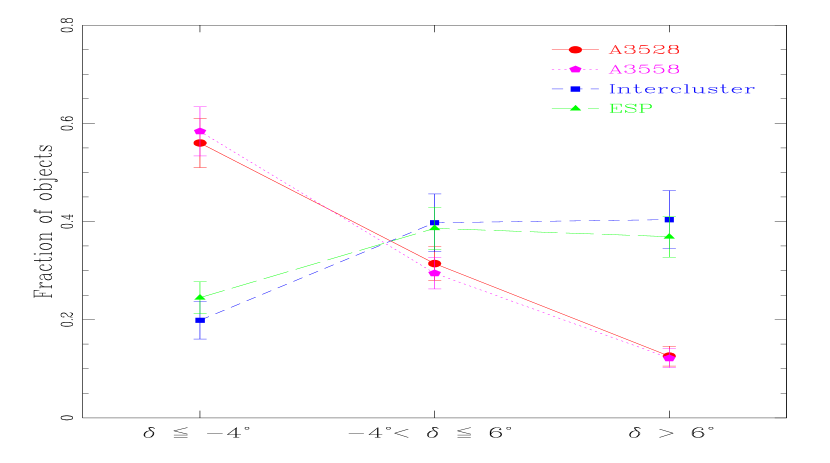
Figure 5: Fractions of galaxies divided in three morphological classes, for each spectral sample: A3528 (circles), A3558 (pentagons), intercluster (squares) and ESP (triangles). The vertical bars represent the 1-$\sigma$ statistical uncertainties.

In Figure 5 the fractions of galaxies in the three morphological bins are shown for each sample. As expected, cluster galaxies show a completely different morphological distribution with respect to ESP and intercluster galaxies, being the fraction of early-type galaxies dominant in such high density environment.
More interesting, this figure shows a broad agreement between the intercluster and the ESP sample: this fact suggests that the galaxies located in the intercluster regions of the Shapley supercluster have a morphological mix not different from field galaxies. This agreement is confirmed also by a more detailed analysis of the histograms of the $\delta$ distributions (Figures 6a and 6b): applying a K-S test, the probability that they have been extracted from the same distribution is more than 40%. Therefore, although the mean overdensity of intercluster galaxies is of the order of $(N/\bar{N})\sim 4$ (Bardelli et al. 2000), their morphological mix has not changed significantly from that corresponding to lower density field galaxies (i.e. ($N/\bar{N})\sim 1$).
For what concerns cluster galaxies, there is a complete agreement between the A3528 and A3558 complex morphological mix (Figure 5). Small differences in the left part of the histograms in Figures 6c and 6d are due to the incompleteness of the A3558 complex survey: literature redshift data (present in the Figure 5 through the use of $(U-B)$ colors but not in the histograms) mainly covers the central region of the A3558 cluster, rich of early-type galaxies. As a consequence of this incompleteness, the $\delta$ distributions of the two complexes are not consistent with the hypothesis of having been extracted from the same distribution: however, limiting the analysis to $\delta>-11^{o}$, the K-S probability rises to $\sim 20\%$.
For what concerns the $\theta$ parameter, it is clear from Figure 3 that a degeneracy is present along the sequence: two galaxy spectra of very different type (for instance an elliptical and an Sc spiral) can have the same value of $\theta$. Given the fact that this parameter is mainly related to the emission line strength, we have analysed the $\theta$ distributions only for late-type galaxies ($\delta>6^{\circ}$). Applying a K-S test to the $\theta$ distributions in each sample, we find that they are all consistent each other. Therefore, although the morphological mix in the cluster environment is significantly different from that in the field, it seems that the spectral properties of the late-type galaxy population do not change in the different environments.

Figure 6: Histograms of the $\delta$ distribution for a) the intercluster sample, b) the ESP sample, c) the A3528 complex, d) the A3558 complex.

5.2 Spectral morphology vs. local density

A more detailed analysis of environmental effects on galaxy morphology can be performed relating the local density with the spectral type. A reliable estimate of the density field is possible only for the cluster complexes: in fact, the sampling of the intercluster region is too sparse and non-uniform to allow a precise description of the local density point by point. For what concerns the ESP galaxies, we consider them as a reference sample with local density consistent with the mean density of the Universe.
For the cluster complexes we have adopted the three-dimensional densities estimated in Bardelli et al. (1998b, 2001) using the DEDICA algorithm (Pisani 1993, 1996). These densities are in units of galaxies per arcmin² per km/s/100: given the fact that the two structures are at different redshifts ($\langle v\rangle$${}_{A3558}\sim 14600$ km/s and $\langle v\rangle$${}_{A3528}\sim 16400$ km/s), it is necessary to rescale the densities in order to allow a meaningful comparison of the samples. We chose to rescale all the values to the A3528 complex, multiplying the A3558 densities by a factor ($\langle v\rangle$${}_{A3528}/$$\langle v\rangle$${}_{A3558})^{2}\sim 1.3$.
For what concerns the A3528 complex, the dynamical and substructure analysis performed in Bardelli et al. (2001) revealed the presence of a number of clumps at $v\sim 20000$ km/s which are not dynamically part of the main structure, mainly associated to the presence of the A3535 cluster. Therefore, we decided to eliminate galaxies with $v\geq 19000$ km/s in the A3528 complex analysis.
We have divided the density range in three bins, roughly equally populated: within these intervals we have calculated the fraction of galaxies with $\delta>2^{\circ}$ and $(U-B)<0.2$ (for literature spectra in the A3558 complex). This value of $\delta$ is located near the boundary between Sa and Sb galaxies (see Figure 3) and therefore we measure the variations with local density of the fraction of intermediate and late spirals and irregulars. The results are shown in Figure 7.

Figure 7: Relation between the fraction of late-type galaxies and local density $f(x,y,z)$ in the A3528 (triangles) and A3558 (squares) complexes, in the magnitude range $17.0\leq b_{J}\leq 18.8$. Horizontal bars indicate the extension of the density intervals: the points are located at the position of the density average value within the bin. Vertical bars represent the 1-$\sigma$ uncertainties. The reference value for the field (from ESP galaxies) is reported as a solid line: dotted lines represent its 1-$\sigma$ uncertainties.

A decreasing of the late-type galaxies fraction with increasing values of density is clearly visible, both in the A3528 and in the A3558 complexes, reflecting the well-known morphology–density relation. Moreover, for every density value, these fractions remain significantly below the mean field value ($53.1\pm 5.3\%$), derived from ESP galaxies and reported as a solid horizontal line in Figure 7. Note that the mean value from intercluster galaxies is very similar ($54.7\pm 7.3\%$).
For what concerns galaxies with $v\geq 19000$ km/s in the A3528 complex, mainly belonging to the poor cluster A3535, there is not a dependence of the morphological mix on the local density: the fraction of late-type spectra remains almost constant (from lower to higher densities: 50%, 48% and 52%) and with values in agreement with those found for the field population. This means that although the densities are rather high, the dynamical mechanisms have not been able to modify the population. This may suggest that A3535 is a young structure, perhaps formed as a consequence of the tidal forces generated by the merging in the A3528 complex.

Looking in more detail at Figure 7 we note that, although the A3528 and the A3558 complexes show a general agreement, the fraction of late-type galaxies at intermediate density is significantly different in the two samples. The A3558 complex distribution appears more regular and smoothly decreasing, while for the A3528 complex there is a sudden drop from the first to the second bin: at intermediate densities the fraction of late-type galaxies is even lower than at high densities (although within the errors). This lack of late-type objects (or, correspondingly, excess of early-type galaxies) is not a consequence of the chosen magnitude bin. Indeed, using the whole sample ($b_{J}\leq 19.5$) we find a morphology-density relation well consistent with the results of Figure 7.
Looking at the spatial distribution of intermediate density early-type galaxies, we find that the excess in the A3528 cluster complex is mainly located in the Southern part, in the A3530-A3532 cluster pair.

Finally, we checked the existence of the morphology-density relation in the complexes considering only galaxies in the regions between clusters, where possibly the shock fronts are located. Although with large error bars, the trend found in these regions is consistent with the global one: taken at face value, this fact seems to be in contradiction with the results of Bardelli et al. (1998b), who found an excess of blue galaxies in the region between A3562 and A3558. However this discrepancy can be understood considering the limited spectral range of our spectra ($\lambda\ga 3700$ Å), which do not allow to fully sample the $U$ band. Looking in detail the spectra of the objects responsible of the blue excess, we find that they are classified as early-type galaxies: the fact that these objects have $(U-B)<0.3$ implies that their spectra have a significant rise in the ultraviolet region (which is outside our spectral range).

6 Equivalent width of [OII] and Star Formation Rate

Other classical properties which are often used to study the galaxy characteristics as a function of the environment are the equivalent width of the [OII]$\lambda 3727$ emission line and the star formation rate. Among the various estimators for the star formation rate we adopted the formula of Kennicutt (1992b), as reported by Balogh et al. (1998)

$$SFR=6.75\times 10^{-12}{{L}\over{L_{\odot}}}EQW({\rm[OII]})\ \ M_{\odot}/yr$$ (8)

where $\displaystyle{{L}\over{L_{\odot}}}$ is the galaxy B-band luminosity normalized to the solar value and $EQW({\rm[OII]})$ is the equivalent width of the [OII] line (in Å). The exact value of the constant, related to the dust absorption, is not relevant in this context because we want to make a comparison between the star formation rates of field and cluster galaxies placed at the same distance.

6.1 Equivalent width of [OII]

We measured the [OII] equivalent width for each galaxy fitting a Gaussian to the [OII] line on the spectrum normalized to its continuum (fitted with a spline3 function). Given the typical signal to noise ratio of our spectra the detection of a line implies an equivalent width larger than about 5 Å. This procedure is the same which was applied to ESP spectra (Zucca et al. 1997).

Analysing the distribution of [OII] equivalent widths in the various samples, we found that the percentage of galaxies with $EQW({\rm[OII]})$$>5$ Å is, as expected, different for field and cluster galaxies, ranging from 44% for the ESP sample and 57% for the intercluster sample, to 14% for the A3528 complex. For the A3558 complex this percentage rises to 31%, but this higher value is a consequence of the fact that the literature redshift data (for which spectra are not available) are mainly concentrated in the core of A3558, rich of early-type galaxies (see also Sect. 4.1): missing the equivalent width measurement of these objects, the fraction of emission line galaxies is artificially increased.

In Figure 8 we show the mean rest frame $EQW({\rm[OII]})$ in the various samples as a function of the local density: as a comparison, the field values are shown as horizontal lines. Note that the mean values were derived considering the total samples, including also galaxies with $EQW({\rm[OII]})$=0. A clear decrease of the mean $EQW({\rm[OII]})$ as the density increases is visible in both cluster complexes, although the values for the A3558 sample are always higher. This fact can be, at least in part, a consequence of the missing spectra of early-type galaxies (see above). Also the cluster A3535 follows a similar trend, but with higher values. Moreover, all these samples are always well below the field: note also that no differences are present between ESP and intercluster galaxies.

We can compare our $EQW({\rm[OII]})$ values with those given by Balogh et al. (1997), who analyzed a sample of 15 rich clusters from the CNOC1 survey, with redshift in the range $0.2-0.55$ and $M_{R}<-18.5$. These authors give the $EQW({\rm[OII]})$ values as a function of the distance from the cluster center: for innermost cluster members ($R<0.3R_{200}$) $\langle EQW({\rm[OII]})\rangle$$=0.3\pm 0.4$ Å, for outer cluster members ($0.3R_{200}<R<2R_{200}$) $\langle EQW({\rm[OII]})\rangle$$=3.5\pm 0.4$ Å, where $R_{200}\sim 1.25$  h^-1 Mpc . Using these limits also for our cluster galaxies, in the same luminosity range of Balogh et al., we find $\langle EQW({\rm[OII]})\rangle$$=0.82\pm 0.61$ Å and $3.28\pm 0.59$ Å for the innermost and outer members, respectively. The very good agreement between our estimates (which refer to low redshift clusters) and those of CNOC1 means that there is no significant evolution in the $\langle EQW({\rm[OII]})\rangle$ value up to $z\sim 0.5$.

Figure 8: Relation between the mean [OII] equivalent width and the local density $f(x,y,z)$ in the A3528 (triangles) and A3558 (squares) complexes, in the magnitude range $17.0\leq b_{J}\leq 18.8$. Open symbols refer to the cluster A3535. Horizontal bars indicate the extension of the density intervals: the points are located at the position of the density average value within the bin. Vertical bars represent the 1-$\sigma$ uncertainties. The reference values for the field are reported as a dotted line (for ESP galaxies) and as a dashed line (for intercluster galaxies).

The dependence of $\langle EQW({\rm[OII]})\rangle$ on the local density can be due to a real intrinsic variation of the line strength with the environment, but can be also simply induced by the existence of a morphology-density relation. In fact, there is a significant correlation between $EQW({\rm[OII]})$ and the classification parameter $\delta$: the highest is the value of $\delta$ for a galaxy, the highest is its line strength.

In order to better investigate this point, we restrict our analysis to late-type galaxies (i.e. with $\delta>2^{\circ}$): in this case, we find that there are no significant variations of $\langle EQW({\rm[OII]})\rangle$ with the local density, for all samples. The mean values, in the whole density range, are: $\langle EQW({\rm[OII]})\rangle$${}_{A3528}=12.71\pm 1.96$ Å, $\langle EQW({\rm[OII]})\rangle$${}_{A3558}=17.64\pm 2.02$ Å, $\langle EQW({\rm[OII]})\rangle$${}_{A3535}=11.87\pm 1.76$ Å, $\langle EQW({\rm[OII]})\rangle$${}_{ESP}=16.63\pm 1.32$ Å and $\langle EQW({\rm[OII]})\rangle$${}_{INTERCL}=15.88\pm 1.58$ Å.
All these values are consistent each other within $2\sigma$ and in some cases already within $1\sigma$: therefore, it seems that the environment has not a strong effect on the line strength of late-type galaxies. This fact confirms the result found using the $\theta$ distribution of late-type galaxies (see Sect. 5.1).

However, to better understand the role of the environment on the galaxy properties we need to take into account also their luminosities, and therefore to analyse their star formation rate.

Figure 9: Relation between the mean star formation rate and the local density $f(x,y,z)$ in the A3528 (triangles) and A3558 (squares) complexes, in the magnitude range $17.0\leq b_{J}\leq 18.8$. Open symbols refer to the cluster A3535. Horizontal bars indicate the extension of the density intervals: the points are located at the position of the density average value within the bin. Vertical bars represent the 1-$\sigma$ uncertainties. The reference values for the field are reported as a dotted line (for ESP galaxies) and as a dashed line (for intercluster galaxies).

6.2 Star Formation Rate

We computed the star formation rate for each galaxy with measured $EQW({\rm[OII]})$, following eq.(8), after having corrected our $b_{J}$ magnitudes for galactic absorption and having transformed them to the B-band.

In Figure 9 we show the mean star formation rate in the various samples as a function of the local density: as a comparison, the field values are shown as horizontal lines. Again the mean values are derived using also galaxies with $SFR=0$. Also in this case there is a clear decrease of the star formation rate with increasing densities, with values well below the field ones. The decrease has a $3.3\sigma$ and $2.6\sigma$ significance level for the A3528 and A3558 samples, respectively. The cluster A3535 is the only exception, being its $\langle SFR\rangle$ higher than the field one and almost independent of the local density.

However, as noted before for the $\langle EQW({\rm[OII]})\rangle$, this behaviour can be induced by the existence of a morphology-density relation: in order to check this point we extrapolated the expected star formation rate for each sample following the method of Balogh et al. (1998).
First we derived from the field sample the mean star formation rate of early-type ($\langle SFR\rangle_{early}$) and late-type ($\langle SFR\rangle_{late}$) galaxies and for each sample we computed in each density bin the fraction of early-type ($f_{early}$) and late-type ($f_{late}$) galaxies. The expected mean star formation rate is then obtained as

$$\langle SFR\rangle=f_{early}\langle SFR\rangle_{early}+f_{late}\langle SFR\rangle_{late}$$ (9)

Note that Balogh et al. (1998) use a photometric classification (bulge or disk dominated) for their galaxies, while we apply a spectroscopic classification ($\delta>2^{\circ}$).

We find that for the cluster complexes the extrapolated $\langle SFR\rangle$ is always higher than the real one, of a factor $\sim 2$ for the A3528 complex and $\sim 1.5$ for the A3558 complex. This trend is qualitatively similar to the results of Balogh et al. (1998), but it has a very low statistical significance ($\sim 1\sigma$): in fact, these authors found a difference of a factor $\sim 5$ between the extrapolated and the real values of the star formation rate.

For what concerns the cluster A3535, we find an opposite behaviour: the extrapolated $\langle SFR\rangle$ is lower than a factor $\sim 0.8$ with respect to the real one, although these two values are consistent each other at $\sim 1\sigma$ level. This fact indicates that in this particular cluster the star formation rate has not been depressed.

7 Discussion and Summary

In this paper we studied the morphological properties of galaxies in the central part of the Shapley Concentration, covering an extremely wide range of densities, from the rich cluster cores to the supercluster environment [$(N/\bar{N})\sim 4$]. Moreover, these results were compared with galaxies from the ESP survey, which represent the reference value for the “true” field [$(N/\bar{N})\sim 1$].

Given the fact that we are using galaxies at the same distance and in a well defined magnitude range, we are not biased by evolutionary effects and by the sampling of different parts of the luminosity function. Moreover, all the spectra in our survey were taken with the same telescope and instrumental set up and therefore our sample is highly uniform. All these characteristics allowed us to perform an accurate spectral classification based on a Principal Components Analysis technique.

We found that all spectra can be well reconstructed using only three components, representing a) an early-type galaxy spectrum, b) a spectrum with very prominent blue continuum and emission lines, and c) an emission line dominated spectrum. This classification can be parametrized using two parameters: $\delta$, which represents the contribution of the blue over the red part of the spectrum, and $\theta$, which represents the importance of the emission lines. In the $\delta-\theta$ plane the galaxies follow a well defined sequence, and it results that $\delta$ is enough to discriminate among the various morphological types.

This spectral classification, together with the [OII] equivalent widths and the star formation rates, has been used to study the properties of galaxies at different densities: cluster, intercluster (i.e. galaxies in the supercluster but outside clusters) and field environment.

The first result is that no significant differences are present between samples at low density regimes (i.e. intercluster and field galaxies): the morphological mix, the $\langle EQW({\rm[OII]})\rangle$ and the $\langle SFR\rangle$ have consistent values in these two environments. This result, although not completely unexpected, has been proved here for the first time.

Cluster galaxies not only have values significantly different from the field ones, but also show a dependence on the local density. A well defined morphology-density relation is present in the cluster complexes: the existence of this relation is not obvious a priori in merging clusters, because the dynamical phenomena could have shuffled galaxies from different local densities.
A possible explanation of the persistence of the relation after a major merging (as in the case of the A3558 complex) is that the shuffling regarded only the peripherical galaxies (i.e. in low density regions), while the cores have potential wells deep enough to retain the original galaxies and to be not influenced by this phenomenon.

Also the $\langle EQW({\rm[OII]})\rangle$ shows a trend with the local environment, decreasing at increasing densities. This trend can be probably induced by the existence of a morphology-density relation: in fact, if we consider only late-type galaxies, we find no significant dependence of $\langle EQW({\rm[OII]})\rangle$ on the local density. Moreover, both field and cluster samples have values consistent each other (within the statistical uncertainties): therefore it seems that the environment has not a strong effect on the line strength of late-type galaxies.

Finally we analyzed the $\langle SFR\rangle$ as a function of the density, finding again a decreasing trend. In order to verify if also this trend is a consequence of the morphology-density relation, we extrapolated the star formation rate expected on the basis of the field $\langle SFR\rangle$ values, taking into account the morphological mix of the clusters [see Sect. 6.2 and eq.(8)]. The extrapolated values are higher than a factor $\sim 1.5-2$ than the observed ones: this result (although with low statistical significance) is consistent with the claim of Balogh et al. (1998) that the star formation rate in clusters is depressed.

Note that the cluster A3535, which is in the background of the A3528 complex, deviates from these trends: it is spiral rich, with a morphological mix similar to the field values, and shows a $\langle SFR\rangle$ consistent with the extrapolated one. This indicates that in this particular cluster the star formation rate has not been depressed.

In this paper we investigated the properties of the galaxy population in a particular, extreme environment: a significant improvement of these studies will be achieved by wide area spectroscopic survey, like 2dFGRS and SDSS, which will allow to homogeneously sample a variety of environments, with high statistics.

References

- [1] Balogh L.M., Morris S.M., Yee H.K.C., Carlberg R.G., Ellingson E., 1997, ApJL 488, L75
- [2] Balogh L.M., Schade D., Morris S.M., Yee H.K.C., Carlberg R.G., Ellingson E., 1998, ApJL 504, L75
- [3] Bardelli S., Zucca E., Vettolani G., Zamorani G., Scaramella R., Collins C.A., MacGillivray H.T., 1994, MNRAS 267, 665
- [4] Bardelli S., Zucca E., Zamorani G., Vettolani G., Scaramella R., 1998a, MNRAS 296, 599
- [5] Bardelli S., Pisani A., Ramella M., Zucca E., Zamorani G., 1998b, MNRAS 300, 589
- [6] Bardelli S., Zucca E., Zamorani G., Moscardini L., Scaramella R., 2000, MNRAS 312, 540
- [7] Bardelli S., Zucca E., Baldi A., 2001, MNRAS 320, 387
- [8] Bellenger R., Dreux M., Felenbok P., Fernandez A., Guerin J., Schmidt R., Avila G., D’Odorico S., Eckert W., Rupprecht G., 1991, The Messenger 65, 54
- [9] Binggeli B., Sandage A., Tammann G.A., 1988, ARA&A 26, 509
- [10] Bothun G.D., 1982, PASP 94, 744
- [11] Butcher H., Oemler A., 1984, ApJ 285, 426
- [12] Connolly A.J., Szalay A.S., Bershady M.A., Kinney A.L., Calzetti D., 1995, AJ 110, 1071
- [13] Dressler A., 1980, ApJ 236, 351
- [14] Felenbok P., Guerin J., Fernandez A., Cayatte V., Balkowski C., Kraan-Korteweg R.C., 1997, Experimental Astronomy 7, 65
- [15] Folkes S., Lahav O., Maddox S., 1996, MNRAS 283, 651
- [16] Fukugita M., Shimasaku K., Ichikawa T., 1995, PASP 107, 945
- [17] Galaz G., de Lapparent V., 1998, A&A 332, 459
- [18] Hoffman G.L., Lewis B.M., Salpeter E.E., 1995 ApJ 441, 28
- [19] Hubble E., Humason M.L., 1931 ApJ 74, 43
- [20] Hubble E., 1936 The Realm of the Nebulae (Oxford, Oxford University Press)
- [21] Kendall M., 1980, Multivariate Analysis, Griffin, London (2nd edition)
- [22] Kennicutt R.C., 1992a, ApJS 79, 255
- [23] Kennicutt R.C., 1992b, ApJ 388, 310
- [24] Lund G., 1986, OPTOPUS - ESO Operating Manual No. 6
- [25] Metcalfe N., Godwin J.G., Peach J.V., 1994, MNRAS 267, 431
- [26] Murtagh F., Heck A., 1987, Multivariate Data Analysis, Reidel
- [27] O’Connell R.W., Marcum P., 1997, in Tanvir N.R., Aragón-Salamanca A., Wall J.V. eds., The Hubble Space Telescope and the high redshift Universe, p. 63
- [28] Postman M., Geller M.J., Huchra J.P., 1984, ApJ 281, 95
- [29] Pisani A., 1993, MNRAS 265, 706
- [30] Pisani A., 1996, MNRAS 278, 697
- [31] Ramella M., Geller M.J., Huchra J.P., 1992, ApJ 384, 396
- [32] Sandage A., 1975, in Sandage A., Sandage M., Kristian J. eds. (Chicago: Univ. Chicago Press), Galaxies and the Universe, 1
- [33] Sodré L.Jr., Cuevas H., 1997, MNRAS 287, 137
- [34] Sodré L.Jr., Cuevas H., Capelato H.V., 1998, in Wide Field Surveys in Cosmology, Colombi S., Mellier Y. eds, Editions Frontieres, p. 424
- [35] de Theije P.A.M., Katgert P., 1999, A&A 341, 371
- [36] de Vaucouleurs G., de Vaucouleurs A., 1961, Mem. R. Astron. Soc. 68, 69
- [37] Yentis D.J., Cruddace R.G., Gursky H., Stuart B.V., Wallin J.F., MacGillivray H.T., Collins C.A., 1992, in MacGillivray H.T., Collins C.A. eds, Digitized Optical Sky Surveys, Kluwer, Dordrecht, p.67
- [38] Vettolani G., Zucca E., Zamorani G. et al., 1997, A&A 325, 954
- [39] Vettolani G., Zucca E., Merighi R. et al., 1998, A&AS 130, 323
- [40] Zaritsky D., Zabludoff A.I., Willick J.A., 1995, AJ 110, 1602
- [41] Zucca E., Zamorani G., Vettolani G. et al., 1997, A&A 326, 477