Finding Galaxy Clusters using Voronoi Tessellations

Abstract

We present an objective and automated procedure for detecting clusters of galaxies in imaging galaxy surveys. Our Voronoi Galaxy Cluster Finder (VGCF) uses galaxy positions and magnitudes to find clusters and determine their main features: size, richness and contrast above the background. The VGCF uses the Voronoi tessellation to evaluate the local density and to identify clusters as significative density fluctuations above the background. The significance threshold needs to be set by the user, but experimenting with different choices is very easy since it does not require a whole new run of the algorithm. The VGCF is non-parametric and does not smooth the data. As a consequence, clusters are identified irrispective of their shape and their identification is only slightly affected by border effects and by holes in the galaxy distribution on the sky. The algorithm is fast, and automatically assigns members to structures.

A test run of the VGCF on the PDCS field centered at $\alpha=13^{h}$ 26^m and $\delta$ = +$29^{o}$ 52’ (J2000) produces 37 clusters. Of these clusters, 12 are VGCF counterparts of the 13 PDCS clusters detected at the 3$\sigma$ level and with estimated redshifts from $z=0.2$ to $z=0.6$. Of the remaining 25 systems, 2 are PDCS clusters with confidence level $<3\sigma$ and redshift $z\leq 0.6$.

Inspection of the 23 new VGCF clusters indicates that several of these clusters may have been missed by the matched filter algorithm for one or more of the following reasons: a) they are very poor, b) they are extremely elongated, c) they lie too close to a rich and/or low redshift cluster.

1 Introduction

Wide field imaging is becoming increasingly common since new large format CCD cameras are, or soon will be available at several telescope (see e.g. MEGACAM, Boulade 1998, Boulade et al. 1998, WFI, Baade 1999, etc). The possibility to perform wide field imaging of the extragalactic sky allows a systematic search of medium-high redshift galaxy clusters in two-dimensional photometric catalogs of galaxies. These candidate clusters are of cosmological interest and are primary targets for subsequent follow-up spectroscopical observations (see, e.g., Holden et al. 1999, Ramella et al. 2000).

Several automated algorithms have already been developed for the detection of clusters within two dimensional galaxy catalogs. The classical techniques used for this task are the “box count” (Lidman & Peterson 1996) and the “matched filter” algorithm proposed by Postman et al. (1996, hereafter P96) and its recent refinements (see Kepner et al., 1999, Kawasaki et al. 1998, Lobo et al 1999).

The box-counting method uses sliding windows (usually squares) which are moved across the point distribution marking the positions where the count rate in the central part of the window exceeds the value expected from the background determined in the outermost regions of the window. The main drawbacks of the method are the introduction of a binning to determine the local background, which improves count statistics at the expense of spatial accuracy, and the dependence on artificial parameters like bin sizes and positions or window size and geometry.

The “matched filter” is a maximum-likelihood (ML) algorithm which analyzes the galaxy distribution with the assumption of some model profiles to fit the data (e.g. a density distribution profile and a luminosity function). This last technique has been used to build the Palomar Distant Cluster Survey (PDCS, see P96) catalog and the EIS cluster catalog (Olsen et al. 1999, Scodeggio et al. 1999). These two catalogs are two of the largest presently available sets of distant clusters, with 79 and 302 candidate clusters respectively.

However, the main drawback of the matched filter method is that it can miss clusters that are not symmetric or that differ significantly from the assumed profile. This can be a serious problem since we know that a large fraction of clusters have a pronounced ellipticity (see e.g. Plionis et al. 1991, Struble & Ftaclas 1994, Wang & Ulmer 1997, Basilakos et al. 2000). Furthermore, the matched filter technique is sensitive to border effects because the ML is computed on a circular area. This is a problem because real galaxy catalogs are finite and usually present holes in regions corresponding to camera defects or bright stars.

Other interesting methods to detect overdensities in a galaxy catalog are the LRCF method (Cocco & Scaramella 1999), kernel based techniques (Silvermann 1986, Pisani 1996), and wavelet transforms (Bijaoui 1993, Fadda et al. 1997). In general, all these techniques are very sensitive to symmetric structures and suffer from border effects.

Ebeling & Wiedenmann (1993) develop a method based on Voronoi tessellation (VTP) in order to identify overdensities in a Poissonian distribution of photon events. Their goal is to detect sources in ROSAT x-ray images. The VTP does not sort points into artificial bins and does not assume any particular source geometry for the detection process. These interesting properties are also very attractive for other applications. For example, Meurs and Wilkinson (1999) present an application of VTP to a slice of the CfA redshift survey with the purpose of isolating the bubbly and filamentary structure of the galaxy distribution. Several other applications of the Voronoi tessellation to astronomical problems have been published (see, e.g., van de Weygaert 2000, El-Ad & Piran 1996, 1997, Ryden 1995, Goldwirth et al. 1995, Zaninetti 1995, Doroshkevich et al. 1997, Ikeuchi & Turner 1991, Icke & van de Weygaert 1991). Clearly, Voronoi tessellation is also interesting for the search of galaxy clusters (Ramella et al. 1999, Kim et al. 2000).

In this paper we present an automatic procedure for the identification of clusters within two-dimensional photometric catalogs of galaxies. Our technique, announced in Ramella et al. 1999, is based on the VTP of Ebeling & Wiedmann (1993). The procedure, hereafter Voronoi Galaxy Cluster Finder (VGCF), is completely non-parametric, and therefore sensitive to both symmetric and elongated and/or irregular clusters. Moreover, the VGCF is not significantly affected by border effects, and automatically assigns members to structures.

Figure 1: Voronoi tessellation of a galaxy field.

Figure 2: Density distribution for the points in Fig. 1 (solid line) and the fitted Kiang distribution (dashed line). The two vertical lines correspond to the 95% and 99% density thresholds for the selection of clusters.

In Sect. 2 we describe the method and in Sect. 3 we show an application of the VGCF to the $\alpha=13^{h}26^{m},\delta=+30^{o}52^{{}^{\prime}}$ field of the Palomar Distant Cluster Survey (see P96). In particular, we illustrate the performances of the algorithm and discuss some aspects of the its application that are specific to the construction of a catalog of galaxy clusters. Finally, in Sect. 4 we summarize our results.

In what follows we assume an Hubble constant $H_{0}=100\,km\,s^{-1}\,Mpc^{-1}$ and a deceleration parameter $q_{0}=1/2$.

2 The method

A Voronoi tessellation on a two-dimensional distribution of points (called nuclei) is a unique plane partition into convex cells, each of them containing one, and only one, nucleus and the set of points which are closer to that nucleus than to any other (see Fig. 1). For us, any point is a galaxy of a given galaxy catalog. The algorithm used here for the construction of the tessellation is the “triangle” C code by Shewchuk (1996). In order to avoid border effects, we restrict our study to Voronoi cells which do not intersect the convex hull of the set of points. In the case of galaxy catalogs with holes, we do not consider Voronoi cells that intersect the hole borders. To do that, we model the hole with a combination of rectangles and we reject cells which have at least one vertex inside one or more of these rectangles.

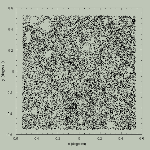
Figure 3: The 25432 galaxies of the PDCS field centered at $\alpha=$ 201.5 degrees and $\delta=$ 29.9 degrees (J2000). Holes correspond to bright stars in the field. North is on the top and East on the left of the figure.

Since we want to find overdensities in a catalog of galaxies, the interesting quantity for us is the density, i.e. the number of galaxies for area unit, rather than the cell area associated by the Voronoi tessellation to each galaxy. An empirical distribution for randomly positioned points following Poissonian statistics, has been proposed by Kiang (1966):

$$dp(\tilde{a})=\frac{4^{4}}{\Gamma(4)}\tilde{a}^{3}e^{-4\tilde{a}}d\tilde{a},$$ (1)

where $\tilde{a}\equiv a/<a>$ is the cell area in units of the average cell area $<a>$. As each cell contains exactly one galaxy the corresponding density is the inverse of the cell area $f\equiv 1/a$. The idea of Ebeling & Wiedenmann (1993) is to estimate the background by fitting the Kiang cumulative distribution to the empirical cumulative distribution resulting from the real catalog in the region of low density which is not affected by the presence of structures ($\tilde{f}\equiv f/<f>\,\leq 0.8$). We can thus establish a density threshold (Fig. 2) and define as overdensity regions those composed by adjacent Voronoi cells with a density higher than the chosen threshold.

In this paper, the density threshold is to separate background regions and fluctuations which are significant overdensities at the 80% c.l.. Since some of the selected overdensities can still be random fluctuations rather than physical clusters, it is necessary to further suppress random overdensities in order to save only significant clusters. We proceed as follows: we compute the probability that an overdensity corresponds to a background fluctuation by:

$$N(\tilde{f}_{min},\leq n)=N_{bkg}\,\frac{\,n_{src,fluc}(\tilde{f}_{min},0)\,e^{-b\tilde{f}_{min}n}}{b(\tilde{f}_{min})},$$ (2)

where $n$ is the number of points associated to the cluster, $N_{bkg}$ is the number of background galaxies, and $\tilde{f}_{min}$ is the minimum normalised density of the cells belonging to the cluster. Both $n_{src,fluc}$ and $b$ are functions of $\tilde{f}_{min}$, which can be computed from simulations (Ebeling & Wiedemann, 1993). We reject overdensities whose probability to be a random fluctuation of the background is greater than 5%.

Figure 4: The solid line is the differential magnitude distribution of galaxies of the PDCS cluster n. 51 ($z_{PDCS}=0.4,N_{R}=80$). The dotted line is the magnitude distribution of average galaxy counts. Counts are normalized to an area of one square degree.

Once we detect significant clusters, we regularize their shape. We assume that the points inside the convex hull defined by the set of points belong to the cluster itself. Then we fit a circle to each cluster and we expand it until the mean density inside the circle is lower than the density of the original cluster. We perform this expansion of the original cluster because the external points of a cluster have usually large area cells, typical of the low density background. These cells can not be associated from the beginning to the cluster by the Voronoi tessellation algorithm.

We stress that fitting a circle to the Voronoi cluster has absolutely no part in the detection of the cluster. It only provides a convenient way to catalog the cluster with a center and a radius. In principle, we could fit an ellipse rather than a circle, since our cluster finder is sensitive to elongated clusters. In practice this is not convenient because, as Ebeling (1993) shows, fitted ellipse eccentricities become insignificant for values lower than about 0.7.

Figure 5: Differential magnitude distribution of galaxies in a circle centered on a simulated cluster at redshift 0.3 and $N_{R}=60$ (solid line). The long dashed line is the magnitude distribution of background galaxies and the short dashed line is the magnitude distribution of cluster galaxies without considering surface brightness selection effects. Counts are normalized to an area of one square degree.

Figure 6: Average number of false detections per field as a function of the threshold in number of coincident fluctuations, $N_{min}$.

At this point we have a list of clusters with position, number of members associated (we statistically subtract the background), contrast against the background, and projected size on the sky. We also have a file of galaxies with position, magnitude, area of the Voronoi tessel, and a label for appartenence to one of the detected clusters. As a final (optional) step, we can assume a density model and fit it on the galaxy distribution at the position where the cluster has been found. In this way we can have a better estimate of the number of members and of the sizes of the cluster, in case clusters are well described by the model.

3 Building a cluster catalog: the case of a PDCS field

In this section we test the VGCF on part of the galaxy catalog used by P96 to produce the Palomar Distant Cluster Survey (PDCS).

In particular, we run the VGCF on the galaxy catalog derived from the $V_{4}$ band image of the PDCS field centered at $\alpha=13^{h}$ 26^m and $\delta$ = +$29^{o}$ 52’ (J2000). The galaxy catalog contains 25432 galaxies. For each galaxy the catalog lists right ascension and declination, and total magnitude in the $V_{4}$ band (see P96, Sect. 2). The effective sky area covered by the field is 1.062 square degrees (see Fig. 3).

We also have a catalog of bright stars areas to be avoided by the VGCF. As already pointed out, the VGCF can very easily deal with “holes” in the galaxy catalog.

3.1 Magnitude bins

The PDCS galaxy catalog is deep, i.e. the number density of galaxies is high. It is therefore a priori possible that only the highest number density contrasts survive the “dilution” caused by foreground/background galaxies. For this reason we decide to run the VGCF in magnitude bins. As we will show, to run the algorithm in magnitude bins also helps in further suppressing spurious clusters.

Figure 7: Average fraction of detections of simulated clusters at z=0.3 (panel a), 0.5 (panel b) and 0.8 (panel c) as a function of $N_{min}$. The different curves in each panel correspond to different values of the richness parameter, $N_{R}$.

The choice of the bin size is somewhat arbitrary and cannot be equally optimal for the detection of all clusters. In fact, the magnitude range of the excess counts produced by clusters varies with the cluster distance and richness. We choose to optimize the bin size for the detection of PDCS-like clusters at intermediate redshift ($z\sim 0.3\,-\,0.6$), i.e around the peak of the galaxy selection function.

In Fig. 4 we plot the magnitude distribution (normalized to unit area) of galaxies within the projected area of P51 ($z_{PDCS}\sim 0.4$ and richness $N_{R}\sim 80$, see P96 for the definition of $N_{R}$), superimposed on the average counts per square degree of the whole PDCS field. From inspection of Fig. 4 it appears that a reasonable choice for the bin size is two magnitudes. With such a bin most of the counts of the cluster peak fall within one bin and the cluster detection is optimal. In fact, a wider bin would decrease the contrast of the cluster counts, while a narrower bin would increase the statistical uncertainty of the detection because of the lower number of cluster counts.

In order to further justify our bin size, we build simulated clusters at different redshifts ($z=$0.3, 0.5 and 0.8 respectively). Our simulated clusters have a projected density profile with a slope $r^{-1}$ outside a core radius of 0.1 Mpc $\,h^{-1}$ and out to a cut-off radius of 1 $\,h^{-1}$ Mpc. This choice is motivated by the fact that PDCS clusters have, on average, a slope $r^{-1.4}$ (Lubin & Postman 1996) and that steeper slopes produce clusters that are more easily detected by the VGCF. We simulate the magnitudes of cluster galaxies by sampling a Schechter luminosity function with a slope $\alpha=-1.2$ and an absolute characteristic magnitude $M_{V}^{*}=-20$. We apply both evolutionary and K-corrections to cluster galaxies according to, respectively, Pence (1976) and Poggianti (1996). We also take into account selection effects in the visibility of galaxies (Phillips et al. 1990). We set the richness of our simulated clusters according to the P96 definition of the richness parameter $N_{R}$ (P96 clusters typically vary from $N_{R}=10$ to $N_{R}=90$). As an example, in Fig. 5, we plot both the counts within the area of a simulated cluster at z=0.3 (radius of 1 Mpc $\,h^{-1}$ and $N_{R}=60$) and the average counts of the PDCS field expected within the same area. From the count distribution of our simulated clusters, we find that a bin size of two magnitudes is indeed adequate to contain the peak of counts corresponding to clusters within the redshift range $z\sim 0.3\,-\,0.6$.

In the case of real clusters, the position of the peak of counts in the magnitude distribution is not known a priori. Therefore, we “slide” at small steps the magnitude bin over the whole magnitude range of the catalog and run the VGCF at each step. We set the step to 0.1 magnitudes, the minimum possible step considering the typical uncertainties of the PDCS magnitudes.

For simplicity, we start the VGCF with the bin $18.0\leq V_{4}<20.0$ and stop at the faint end of the survey, i.e. with the bin $21.8\leq V_{4}<23.8$. We neglect 76 galaxies brighter than $V_{4}=18.0$ without consequences for our identification of clusters within the redshift range $z\sim 0.3\,-\,0.6$.

3.2 Clusters and their detections in bins

Before producing our final cluster catalog, we need to define a criterium to identify clusters by associating fluctuations detected in different magnitude bins. The criterium will consists of a maximum projected distance between the centers of fluctuations to be associated and of a minimum number of coincident fluctuations required for a positive detection, $N_{min}$. In fact, because of the statistical noise of the foreground/background galaxy distribution, the centers of the fluctuations produced by a cluster in different magnitude bins will be slightly different. As far as the number of coincident fluctuations produced by a cluster is concerned, it will depend on the cluster distance, richness and luminosity function. Clearly the choice of the criterium has to be made having in mind the goal of the detection algorithm and the characteristics of the galaxy catalog.

Table 1: The cluster catalog

N	A.R. (deg.)	Decl. (deg.)	R (arcsec.)	Contrast	Ncl	Nbg	Mag. bin	Remarks
V1	201.623	29.977	227	7.91	25	10	4 (19.4)	P55
V2	201.546	29.412	162	7.27	23	10	9 (19.9)	P49
V3	201.437	29.492	133	4.47	10	5	11 (20.1)	-
V4	201.595	29.559	216	9.22	69	56	31 (22.1)	P50
V5	201.695	30.043	112	5.50	11	4	13 (20.3)	-
V6	201.351	30.291	144	5.37	12	5	9 (19.9)	-
V7	201.095	29.783	58	6.36	9	2	30 (22.0)	-
V8	200.931	29.592	162	7.51	39	27	24 (21.4)	P51
V9	201.381	29.640	137	9.65	32	11	26 (21.6)	P52
V10	200.915	30.376	90	10.67	32	9	27 (21.7)	P62
V11	201.498	30.365	155	5.81	26	20	21 (21.1)	-
V12	201.247	29.720	115	6.01	19	10	22 (21.2)	P53
V13	201.549	29.928	61	6.00	6	1	21 (21.1)	-
V14	201.427	29.569	65	7.00	7	1	14 (20.4)	-
V15	201.079	29.918	151	4.67	14	9	21 (21.1)	-
V16	201.842	29.382	61	7.00	7	1	19 (20.9)	P46
V17	201.910	30.094	101	6.64	23	12	28 (21.8)	P58
V18	201.636	29.450	176	8.95	31	12	22 (21.2)	-
V19	201.603	29.845	115	6.00	12	4	23 (21.3)	-
V20	201.515	29.649	122	5.37	24	20	27 (21.7)	-
V21	201.278	30.409	104	6.15	23	14	30 (22.0)	P15
V22	201.733	30.348	112	7.25	29	16	27 (21.7)	-
V23	200.935	29.678	108	6.50	13	4	22 (21.2)	-
V24	200.957	29.451	148	6.15	23	14	22 (21.2)	-
V25	201.836	29.856	68	6.05	16	7	34 (22.4)	-
V26	201.941	30.184	115	6.10	22	13	29 (21.9)	-
V27	201.942	29.550	72	6.35	11	3	26 (21.6)	-
V28	201.776	30.005	72	5.77	10	3	28 (21.8)	P56
V29	201.935	29.500	79	5.50	11	4	29 (21.9)	-
V30	201.469	30.218	122	5.72	14	6	30 (22.0)	-
V31	200.959	29.359	97	5.55	20	13	32 (22.2)	P47
V32	202.105	30.145	115	6.01	19	10	28 (21.8)	-
V33	201.866	30.140	68	5.00	10	4	28 (21.8)	-
V34	200.941	30.057	86	5.81	13	5	29 (21.9)	P57
V35	200.906	30.080	68	6.00	12	4	38 (22.8)	-
V36	201.091	30.211	83	6.33	21	11	37 (22.7)	P63
V37	200.983	30.108	111	5.63	27	23	38 (22.8)	-

Figure 8: Clusters detected by the VGCF (solid circles) and by by the matched filter algorithm (dotted circles). VGCF identification numbers are at the center of the solid circles, PDCS identification numbers are on the side of dotted circles. The field is centered at $\alpha=$ 201.5 degrees and $\delta=$ 29.9 degrees (J2000). North is on the top and East on the left of the figure.

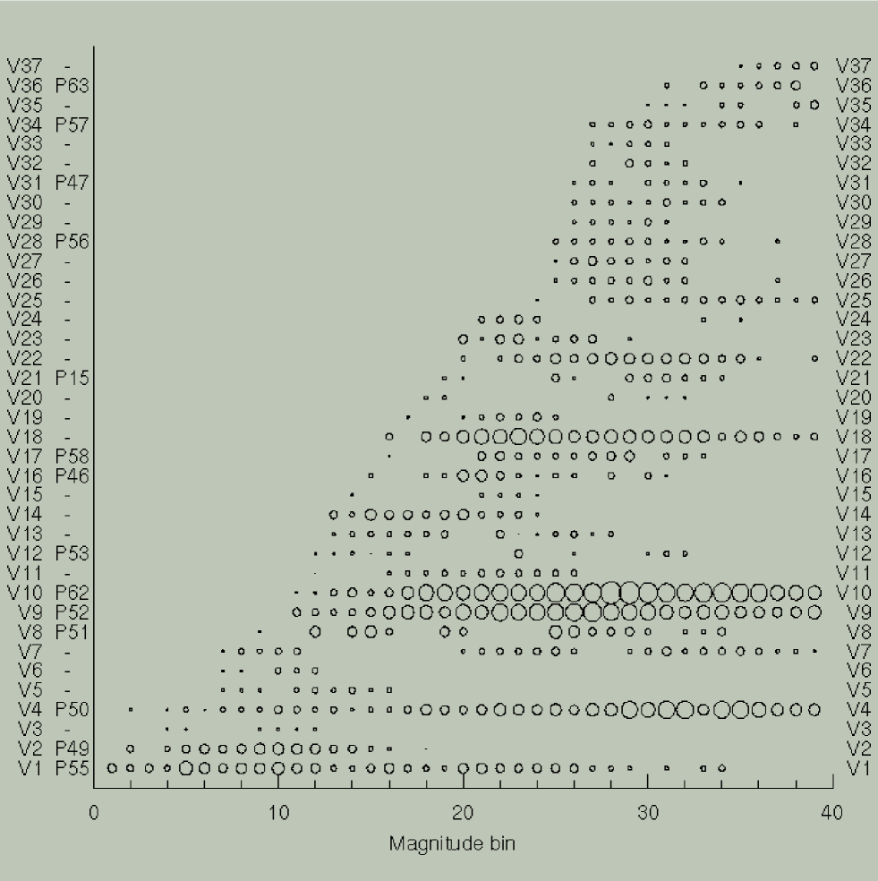
Figure 9: Plot of the density contrast of clusters detected by VGCF in 39 magnitude bins. Radii are scaled with the signal-to-noise ratio of the detection. The labels on the left of the figure are the VGCF and the PDCS identification numbers respectively.

In order to define the criterium of association for our test application, we peform extended tests both on the PDCS field and on simulations of Poissonian fields with embedded simulated clusters. Our simulated fields have the same general properties of the PDCS field. In particular, we run the VGCF on 100 catalogs each containing 18 simulated clusters (a number similar to the number of clusters in the PDCS field) embedded within a Poissonian galaxy field. Clusters are simulated as in the previous subsection. All simulated catalogs contain 25432 galaxies, i.e. the same number of PDCS galaxies.

As a result of our tests, we consider coincident two fluctuations with centers separated on the sky by a projected distance $d_{12}\leq 0.3\,min(R_{1},R_{2})$, where $R_{1}$ and $R_{2}$ are the radii of the two fluctuations. A tighter criterium would break the sequence of fluctuations corresponding to a real cluster, a looser criterium would incorrectly associate fluctuations produced by adjacent clusters/fluctuations to the same cluster.

We now set the minimum number of fluctuations, $N_{min}$, required for the detection of a cluster. In Fig. 6 we plot the average number of spurious fluctuations mis-identified as clusters as a function of $N_{min}$. The number of spurious clusters drops dramatically as $N_{min}$ increases from 1 to 5. For $N_{min}=5$ there are on average 1.5 spurious clusters per field. This number decreases slowly as $N_{min}$ increases further. This result indicates that $N_{min}=5$ is a a good choice to keep the number of Poisson fluctuations low while still being sensitive to poor or distant clusters.

In Fig. 7 we show the variation with $N_{min}$ of the detection efficiency of simulated clusters at redshifts z=0.3 (panel a), 0.5 (panel b), and 0.8 (panel c). At each redshift the different curves correspond to richnesses ranging from $N_{R}=10$ to $N_{R}=60$. Clearly the fraction of detected clusters decreases as $N_{min}$ increases.

We note that the curve in Fig. 6 corresponds to an evaluation of the False Positive Rate (FPR), i.e. the probability of detecting as a cluster a random fluctuation of the galaxy distribution. For $N_{min}=5$, our FPR is very low. By comparison, P96 give 4.2 spurious detections per square degree with peak signal greater than $3\sigma$. The curves in Fig. 7 correspond to a measure of the False Negative Rate (FNR).

3.3 The VGCF run and comparison with P96

We present here the results of the run of the VGCF on the $V_{4}$ catalog of the PDCS field at $\alpha=13^{h}$ 26^m and $\delta$ = +$29^{o}$ 52’ (J2000). As discussed in the previous section, we run the VGCF in bins two magnitude wide, “sliding” with 0.1 magnitude steps within the magnitude range $18.00\leq V_{4}<23.8$. In total we run the VGCF in 39 magnitude bins and identify as clusters at least five fluctuations that, according to our criterium, are angularly coincident (see previous subsection).

On a Sun ULTRASparc 30 workstation, the time required to run the whole procedure is about 40 minutes.

Our output cluster list consists of 37 objects. We characterize each cluster with the properties of the fluctuation with the highest signal-to-noise ratio as estimated by the ratio of the number of cluster galaxies to the square root of the number of background galaxies expected within the cluster area.

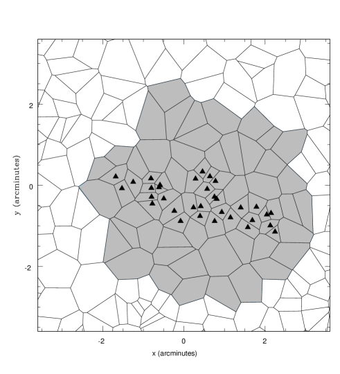
Figure 10: Plot of the galaxies of cluster V26 detected by the VGCF in the bin of maximum contrast before regularization processes (black triangles). The grey cells are those of galaxies added at the end of the regularization processes. Empty cells are those of background galaxies. North is on the top and East on the left of the figure.

Figure 11: Richness distribution of P96 clusters as detected by the VGCF (dotted line) and of new VGCF clusters (solid line).

In Table 1, for each cluster we list: 1) identification number, 2) J2000 right ascension and 3) J2000 declination, 4) radius, 5) the cluster signal-to-noise ratio, 6) the estimated number of cluster galaxies and 7) the number of expected background galaxies, 8) the central magnitude of the bin where we detect the cluster with the highest signal-to-noise ratio, 9) the cross-identification with the PDCS catalog.

In Fig. 8 we plot circles on the sky corresponding to our clusters (solid lines). We label our clusters with a “V” followed by their order number in Table 1. In Fig. 9, we give a graphic summary of all the fluctuations of each cluster. The abscissa is the order number of the magnitude bin of the fluctuation and each cluster is represented by a row of circles parallel to the magnitude bin axis. The radii of the circles are scaled with the signal-to-noise ratio of the detection.

We remind here that we fit a circle to a fluctuation after its detection, and that the only use of the circle is to provide a convenient way to catalog the cluster with a center and a radius.

The richest and more reliable clusters exhibit, in Fig. 9, a sequence of fluctuations. The signal-to-noise ratio of these fluctuations regularly increases up to a maximum and then decreases. Several fainter clusters show the same behavior, although at a generally lower S/N level. Clearly, the position of the fluctuations along the magnitude axis is related to the cluster distance.

Some clusters, for example V7 and V12, display substantial gaps along the sequence. The suspicion is that these clusters may actually consist of unrelated overdensities projected along the same line-of-sight.

We now proceed to a detailed comparison with P96 clusters. The original PDCS catalog consists of 19 clusters detected by the matched filter algorithm both in the $V_{4}$ band and in the $I_{4}$ band (see P96, Table 4). Furthermore, the PDCS catalog lists 7 clusters detected only in the $V_{4}$ band and added to the catalog after visual inspection of the CCD images (see P96, Table 5). In total there are 26 P96 $V_{4}$-band clusters, 18 of which are detected at the 3$\sigma$ level. Of these last clusters, 13 have estimated redshift within the range where our VGCF is optimal ($0.2\leq z\leq 0.6$). In Fig. 8 we plot circles corresponding to all the P96 clusters detected by the matched filter technique (dotted line).

We identify 12 of the 13 clusters detected by P96 at the 3$\sigma$ level and with estimated redshifts from $z=0.2$ to $z=0.6$. The only cluster we do not identify, P54 ($z=0.5$), falls just under the limit of our selection criterium with only four coincident fluctuations.

Beside the above 12 clusters, we detect other 25 galaxy systems. Of these 25 systems, 2 are P96 clusters with confidence level less than 3$\sigma$ and redshift $z\leq 0.6$. The remaining 23 do not have a counterpart in the PDCS catalog.

Most of the 23 new clusters have properties comparable to those of P96 clusters as detected by the VGCF. At least part of the new systems have been detected by the VGCF thanks to its specific properties. For example, because the VGCF does not smooth the data, it is able to separate two large overdensities (V2 and V18) that are unlikely to be one system (P49). In fact V2 (which we identify as the counterpart of P49) and V18 are well separated both on the sky and in magnitude.

The property of the VGCF of detecting overdensities irrespective of their shape is probably the key for the detection of V26, a very elongated system. In Fig. 10 we show the galaxies of V26 as detected by the VGCF before the regularization processes (black triangles). We also show as grey tessels those of galaxies added at the end of the regularization processes and as white tessels those of background galaxies. The plot refers to the tessellation of the PDCS field in the magnitude bin of maximum contrast for V26.

As far as the richness, $N_{R}$, of VGCF clusters is concerned, we compute it almost in the same way as P96, the only difference being that we use a fixed angular radius of 0.1 deg within which to count cluster galaxies. For systems within the redshift range 0.3-0.6, our angular radius roughly corresponds to a linear radius of 1 $\,h^{-1}$ Mpc. As P96 shows, $N_{R}$ is related to the Abell richness of the system.

In Fig. 11 we plot the distribution of $N_{R}$ of our new systems (solid histogram) and of P96 clusters as detected by the VGCF (dotted histogram). In general the richness of the new systems is similar to that of P96 clusters (as detected by the VGCF), but the VGCF detects a larger fraction of poor systems than the matched filter algorithm. In fact, we have 5 systems with $N_{R}<20$ while only 1 P96 cluster falls within this range. We probably find these poorer systems because we do not smooth the data.

That the general properties of new VGCF systems are not very different from P96 systems is also evident from Fig. 11 where we label with a “P” and the PDCS identification number the VGCF identifications of P96 clusters.

A more detailed comparison between our and P96 clusters is not useful since, in the end, only spectroscopic observations will allow a real comparison between the performances of the two algorithms. What we would like to stress here is that the VGCF is an algorithm that can usefully complement the matched filter (and probably other parametric cluster searches) for the definition of a complete and reliable 2D cluster catalog.

In many problems we think that the VGCF could be preferred over parametric searches and, in these cases, the example we discuss in this section shows that the VGCF retrieves most of the reliable identifications of the parametric searches.

4 Summary

We present an objective and automated procedure for detecting clusters of galaxies in imaging galaxy surveys. Our Voronoi Galaxy Cluster Finder (VGCF) uses galaxy positions and magnitudes to find clusters and determine their main features: size, richness and contrast above the background. The VGCF uses the Voronoi tessellation to evaluate the local density and to identify clusters as significative density fluctuations above the background. The significance threshold needs to be set by the user, but experimenting with different choices is very easy since it only requires a new selection from the output of the Voronoi tessellation and not a whole new run of the algorithm. The VGCF is non-parametric and does not require a smoothing of the data. As a consequence, clusters are identified irrispective of their shape and their identification is only slightly affected by border effects and by holes in the galaxy distribution on the sky.

The algorithm is fast, and automatically assigns members to structures. For example, a run on about 25000 galaxies only requires 7 minutes on a Sun ULTRASparc 30 workstation.

We perform test runs of the VGCF both on simulated galaxy fields and on the 25432 galaxies identified in the $V_{4}$ band image of the PDCS field centered at $\alpha=13^{h}$ 26^m and $\delta$ = +$29^{o}$ 52’ (J2000, see P96). Given the depth of the PDCS survey, we run the VGCF in 39 overlapping 2 magnitude wide bins, from $V_{4}=18.00$ to $V_{4}=23.75$. For the detection of a cluster we require at least five angularly coincident fluctuations. Based on 100 simulations of the PDCS field, we find that there are, on average, 1.5 spurious detections in a simulated PDCS field with Poisson background. Our choice of bin size and number of bins, together with the minimum number of fluctuations required for a cluster detection, optimizes the VGCF for the redshift range $0.3\mathrel{\hbox{\hbox to0.0pt{\hbox{\lower 4.0pt\hbox{$\sim$}}\hss}\hbox{$<$}}}z\mathrel{\hbox{\hbox to0.0pt{\hbox{\lower 4.0pt\hbox{$\sim$}}\hss}\hbox{$<$}}}0.6$.

We find 37 clusters, 12 of which are VGCF counterparts of the 13 PDCS clusters detected at the 3$\sigma$ level and with estimated redshifts from $z=0.2$ to $z=0.6$. Of the remaining 25 systems, 2 are P96 clusters with confidence level $<3\sigma$ and redshift $z\leq 0.6$.

23 VGCF clusters have no counterpart in the PDCS catalog. An inspection of their properties indicates that some of these clusters may have been missed by the matched filter algorithm for one or more of the following reasons: a) they are very poor, b) they are extremely elongated, c) they lie too close to a rich and/or low redshift cluster.

In conclusion, the VGCF can usefully complement the matched filter algorithm (and probably other parametric cluster searches) for the definition of a complete and reliable 2D cluster catalog. In fact, we think that the VGCF could be preferred over parametric searches in many cases since the example we discuss shows that the VGCF anyway retrieves the reliable identifications of parametric searches.

- (1) Baade D., 1999, LSO-MAN-ESO-22100-00001
- (2) Basilakos S., Plionis M., Maddox S.J., 2000, MNRAS 316, 779
- (3) Bijaoui A., 1993, in Wavelets, Fractals, and Fourier Transforms, Farge M., Hunt J.C.R. & Vassilicos J.C. (eds.). Oxford Univ. Press, p. 195
- (4) Boulade O., 1998, Experimental Astronomy, v. 8, Issue 1, 25
- (5) Boulade O., Vigroux L.G., Charlot X. et al., 1998, Proc. SPIE Vol. 3355, “Optical Astronomical Instrumentation”, D’Odorico S., ed., p. 614-625
- (6) Cocco V.,Scaramella R., 1999, in “Observational Cosmology: The Development of Galaxy Systems”, Sesto Pusteria, Italy, 30 June - 3 July, 1998, Eds.: G. Giuricin, M. Mezzetti, & P. Salucci, PASPC 176, 97
- (7) Doroshkevich A.G., Gottlober S., Madsen S., 1997, A&AS 123, 495
- (8) Ebeling H., 1993, MPE report 250 (ISSN 0718-0719)
- (9) Ebeling H., Wiedenmann G., 1993, Ph. Rev. E 47, 704
- (10) El-Ad H., Piran T., 1996, ApJ 462, L13
- (11) El-Ad H., Piran T., 1997, ApJ 491, 421
- (12) Fadda D., Slezak E., Bijaoui A., 1997, A&A 127, 335
- (13) Goldwirth D.S., da Costa L.N., van de Weygert R., 1995, MNRAS 275, 1185
- (14) Holden B.P., Nichol R.C., Romer A.K., Metevier A., Postman M., Ulmer M.P., Lubin L.M., 1999, AJ 118, 2002
- (15) Icke V., van de Weygaert R., 1991, RASQJ 32, 85
- (16) Ikeuchi S., Turner E.L., 1991, MNRAS 250, 519
- (17) Kawasaki W., Shimasaku K., Doi M., Okamura S., 1998, A&AS 130, 567
- (18) Kepner J., Fan X., Bahcall N., Gunn J., Lupton R., Xu G., 1999, ApJ 517, 78
- (19) Kiang T., 1966, Zeitschrift für Astrophysik 64, 433
- (20) Kim R.S.J. et al., 2000, in “Clustering at high redshift”, Les Rencontres Internationales de l’IGRAP, Marseille, France, July 1999, Eds., A. Mazure, O. Le Fevre, & V. Lebrun, PASPC 200, 422
- (21) Lidman C.E., Peterson B.A., 1996, AJ 112, 2454
- (22) Lobo C., Lazzati D., Iovino A., Chincarini G., 1999, in “Wide Field Surveys in Cosmology”, 14th IAP meeting held May 26-30, 1998, Paris. Publisher: Editions Frontieres. ISBN: 2-8 6332-241-9, p. 239.
- (23) Lubin L.M., Postman M., 1996, AJ 111, 1795
- (24) Meurs E.J.A., Wilkinson M.I., 1999, in “Observational Cosmology: The Development of Galaxy systems”, Sesto Pusteria, Italy, 30 June - 3 July, 1998, Eds.: G. Giuricin, M. Mezzetti, & P. Salucci, PASPC 176, 333
- (25) Olsen E. et al., 1999, A&A 345, 363
- (26) Pence W., 1976, ApJ 203, 39
- (27) Phillips S., Davies J.I., Disney M.J., 1990, MNRAS 242, 235
- (28) Pisani A., 1996, MNRAS 278, 697
- (29) Plionis M., Barrow J.D., Frenk C.S., 1991, MNRAS 249, 662
- (30) Poggianti B., 1996, A&AS 122, 399
- (31) Postman M., Lubin L., Gunn J.E., Oke J.B., Hoessel J.G., Schneider D.P., Christensen J.A., 1996, AJ 111, 615 (P96)
- (32) Ramella M., Nonino M., Boschin W., Fadda D., 1999, in “Observational Cosmology: The Development of Galaxy Systems”, Sesto Pusteria, Italy, 30 June - 3 July, 1998, Eds.: G. Giuricin, M. Mezzetti, & P. Salucci, PASPC 176, 108
- (33) Ramella M., Biviano A., Boschin W., Bardelli S., Scodeggio S., Borgani S., Girardi M., da Costa L., Olsen E., Nonino M., 2000, A&A 360, 861
- (34) Ryden B.S., 1995, ApJ 452, 25
- (35) Scodeggio M. et al., 1999, A&AS 137, 83
- (36) Shewchuk J.R., 1996, in “First Workshop on Applied Computational Geometry”, ACM (http://www.cs.cmu.edu/quake/triangle.html)
- (37) Silvermann B.W., 1986, Density Estimation for Statistics and Data Analysis. Chapman & Hall, New York
- (38) Struble M.F., Ftaclas C., 1994, AJ 108, 1
- (39) van de Weygaert R., 2000, in “Large Scale Structure in the X-ray Universe”, Proceedings of the Workshop held in Santorini, Greece, September 1999, eds. M. Plionis & I. Georgantopoulos, Atlantisciences, Paris (France), p.135
- (40) Wang Q.D., Ulmer M.P., 1997, MNRAS 292, 220
- (41) Zaninetti L., 1995, A&AS 109, 71