Diffraction-limited 800nm imaging with the
2.56m Nordic Optical Telescope

A quantitative assessment is presented of diffraction-limited stellar images with Strehl ratios of 0.25-0.30 obtained by selection of short-exposure CCD images of stars brighter than +6m at 810nm with the Nordic Optical Telescope.

1 Introduction

The selection of the few sharpest images from a large dataset of short exposures provides one method of obtaining high resolution images through atmospheric seeing at ground-based telescopes. The selected exposures can then be processed using one of the conventional speckle techniques such as shift-and-add. Exposure selection has been applied in many studies of the solar surface and for planetary imaging but has not been extensively tested as a general tool for astronomical imaging at optical wavelengths. Trials by Dantowitz (1998) and Dantowitz et al. (2000) using a video camera on the 60-inch Mt.Wilson telescope have shown its promise for reaching close to the diffraction limit. In view of the technical difficulties of adaptive optics at wavelengths shorter than 1 $\mu$m, it seems important to assess this alternative technique quantitatively. In this paper we present such observations, showing the power of the method and argue that new developments in low-noise, fast-readout CCD’s make it attractive for achieving diffraction-limited imaging in the visible waveband for faint astronomical targets using apertures of about 2.5m.

The basis for the method is that the atmosphere behaves as a time-varying random phase screen, with a power spectrum of irregularities characterised by spatial and temporal scales $r_{0}$ and $t_{0}$, whose rms variations are larger than those of a well-adjusted and figured primary mirror. Occasionally the combined phase variations across the telescope aperture, $\delta$, due to the atmosphere and mirror, will be small ($<\sim 1$radian). The corresponding image of a star will have a core which is diffraction-limited with a Strehl ratio of $\exp{(-\delta^{2})}$ and angular resolution $1.22\lambda/D$ determined by the aperture diameter $D$. Fried (1978) calculated the probability, $P$, of “lucky exposures” having phase variations less than 1 radian across an aperture diameter $D$ for seeing defined by $r_{0}$:

$$P\simeq 5.6\exp{\left(-0.1557\left(D/r_{0}\right)^{2}\right)}$$

This implies, for instance, that for an aperture $D=7r_{0}$, one exposure in 350 would have a Strehl ratio greater than 0.37. For $D=10r_{0}$, the frequency of such good exposures falls to only one in $10^{6}$. This suggests that values of $D$ chosen as $7r_{0}$ may offer the best compromise between high angular resolution and frequency of occurrence.

The technique evidently requires a site with good seeing and a telescope for which it is known that the errors in the mirror figure are small compared with the atmospheric fluctuations on all relevant scales. The primary mirror should ideally match the maximum useful aperture for this technique. If very good seeing is taken to be 0.5 arcsec, and a useful aperture as $7r_{0}$, then D should be 1.4m at 500nm and 2.5m at 800nm. The Nordic Optical Telescope (NOT) matches these criteria very closely.

2 Observations and Data Reduction

Observations were made at the Cassegrain focus of the NOT on the nights of 2000 May 12 and 13. The camera was one developed for the JOSE programme of seeing evaluation at the William Herschel Telescope (St-Jacques et al. 1997). It comprised a 512x512 front illuminated frame-transfer CCD with 15 $\mu$m pixels run by an AstroCam 4100 controller. The controller allows windowing of the area of readout and variable pixel readout rates up to 5.5MHz. The f/11 beam at the focus was converted to f/30 using a single achromat to give an image scale of 41 milliarcsec/pixel (25 pixels/ arcsec). This gives a good match to the full width to half maximum (FWHM) of the diffraction-limited image of 66 milliarcsec for a 2.56m telescope with 0.50m secondary obstruction at 800nm; good signal-to-noise sensitivity per pixel is retained whilst the resolution is degraded only slightly to 77 milliarcsec FWHM by the finite pixel size.

A filter centred at 810nm with a bandwidth of 120nm was used to define the band. All of the exposures of stars were taken at frame rates higher than 150Hz and without autoguiding to ensure that the temporal behaviour of the periods of good seeing was adequately characterised.

Observations of the stars listed in Table 1 were made with a variety of frame formats and frame rates. Each run typically comprised between 5000 and 24000 frames over a period of 30-160s. Target stars, both single stars and binaries, were chosen principally lying in the declination range $10\degr$-$20\degr$ and close to the meridian, so that most of the data was taken at zenith angles $<20\degr$. Zenith angles up to $50\degr$ were explored in later observations. The effects of atmospheric dispersion became significant, since no corrective optics were employed.

Table 1: Observations

$$\begin{array}[]{p{0.25\linewidth}p{0.3\linewidth}l}\hline\cr\vskip 3.0pt plus 1.0pt minus 1.0pt\cr Target&Frame rate / Hz&FWHM/arcseconds\\ \vskip 3.0pt plus 1.0pt minus 1.0pt\cr\hline\cr\vskip 3.0pt plus 1.0pt minus 1.0pt\cr v656 Herculis&185&0.49\\ $\epsilon$ Aquilae&185&0.38\\ $\gamma$ Aquilae&185&0.46\\ $\gamma$ Leonis&159&0.57\\ $\gamma$ Leonis&182&0.46\\ CN Bo\"{o}tis&152&0.62\\ $\zeta$ Bo\"{o}tis&152&0.74^{\mathrm{a}}\\ $\zeta$ Bo\"{o}tis&152&0.75^{\mathrm{a}}\\ $\alpha$ Herculis&191&0.38\\ $\alpha$ Aquilae&206&0.50\\ $\beta$ Delphini&373&0.42\\ $\beta$ Delphini&257&0.52\\ $\beta$ Delphini&190&0.64\\ $\alpha$ Delphini&180&0.41\\ $\alpha$ Delphini&180&0.49\\ \vskip 3.0pt plus 1.0pt minus 1.0pt\cr\hline\cr\end{array}$$

• Includes some tracking error

The seeing was good, typically 0.5 arcsec (see Table 1), and the short exposure images seen in real time clearly showed a single bright speckle at some instants. The full aperture of the NOT was therefore used for all the observations on both nights.

The analysis of the data was carried out in stages:

1. Some runs in which the detector was saturated during the periods of best seeing and a small number of misrecorded frames in runs taken at the fastest frame rates were excluded from further analysis.

2. For each run, an averaged image was obtained by summing all the remaining frames. The mean sky level was measured from a suitable area of the image and subtracted before determining the FWHM of the seeing disk (Table 1) and the total stellar flux.

3. Each frame was interpolated to give a factor of 4 times as many pixels in each coordinate using sinc interpolation to overcome problems of sampling in the images.

4. The peak brightness and position of the brightest pixel in each frame was measured and stored.

5. The Strehl ratio for each frame was derived using the peak brightness above the sky level measured for that frame, scaled by the total flux from the star and a geometrical factor which relates the pixel scale to the theoretical diffraction response of the NOT.

6. A “good” image was then obtained by taking only those frames with a Strehl ratio greater than some chosen value, shifting the images so that the peak pixels were superposed and adding the frames.

Fig. 1 shows a histogram of the Strehl ratios derived following 1-5 above for individual 5.4 ms exposures in a 32 second run on the star $ϵ$ Aquilae. The substantial improvement in the Strehl of the shift-and-add image and in limiting sensitivity provided by image selection is clear from the spread of the Strehl values. For comparison, a histogram is also plotted of the Strehl ratios obtained for images from simulations of 10,000 realisations of atmospheric irregularities with a Kolmogorov turbulent spectrum over a circular aperture $6.5r_{0}$ in diameter. The close agreement between theory and observation suggests that the conditions corresponded to $6.5r_{0}$ = 2.56m at 810nm for this run. The FWHM of the averaged image from this run was 0.4 arcsec, corresponding to the telescope aperture being only $5.8r_{0}$ for a Kolmogorov spectrum of turbulence. The discrepancy is partly explained by the actual image motion being only 60% of that for a Kolmogorov spectrum, implying an outer scale of turbulence of about 30m.

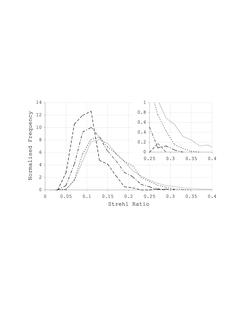
Figure 1: Histogram of the Strehl ratios calculated for 5950 exposures of $ϵ$ Aquilae taken over a period of $\sim$30 seconds. The dotted curve shows the measured distribution of Strehl ratios for the individual exposures. The solid line is for a computer simulation of Kolmogorov turbulence with an aperture diameter of $6.5r_{0}$. The dot-dashed curve shows the Strehl ratios which result after averaging together groups of five consecutive exposures of $ϵ$ Aquilae without correction for image motion. If groups of 20 consecutive exposures are averaged together the resulting images typically have substantially lower Strehl ratios (dashed line). For this case only one of the averaged images gives a Strehl greater than 0.25.

The timescale on which changes take place in the best images is an important question, setting a limit to the maximum frame exposure time which can be used in this technique, and hence to the faintest limiting magnitude achievable with a given camera. Histograms of the Strehl ratios obtained after averaging together groups of 5 successive frames without correction for image motion are included in Fig. 1. This shows that exposures as long as 30ms could be used with only a small reduction in the observed Strehl values. The Strehls are reduced substantially if 20 exposures are averaged together. The choice of best exposure time depends on the intended application.

3 Results

Data from the run on $ϵ$ Aquilae analysed in several different ways illustrate the possible strategies in practice. Fig. 2a shows a 108ms exposure, formed by the summation without shifting of 20 consecutive 5.4 ms exposures, during a single period of good atmospheric conditions. The FWHM of the central core in the image is 79$\times$95 milliarcseconds, with a Strehl ratio of 0.29. Fig. 2b was constructed from 12 exposures of 27ms duration, each made by summing without shifting five 5.4ms exposures. These 12 exposures were shifted and added to give a final FWHM of 81$\times$96 milliarcseconds and a Strehl ratio of 0.26. Single 5.4ms exposures from 20 widely separated time periods were selected for Fig. 2c. Each of the constituent exposures had a Strehl ratio greater than 0.27, resulting in an image core with 80$\times$93 milliarcseconds FWHM and a Strehl of 0.30 after shifting and adding. For Fig. 2d the exposures with the highest 1% of Strehl ratios are selected, giving a final image with FWHM of 79$\times$94 milliarcseconds and Strehl ratio of 0.30. All of these procedures give images with high Strehl ratios. There is, however, a trade-off between the higher sensitivity for faint reference stars achieved by the long sequence in Fig. 2a and the smoothness of the halo due to averaging many atmospheric configurations as in Fig. 2. b-d. For the remainder of this letter we have used the best 1% of exposures in any observation to produce the final image.

Figure 2: a-d. Image quality of $ϵ$ Aquilae using differing criteria for exposure selection from a 32s run. Contour levels are at 1, 2, 4, 8, 16, 30, 50, 70, 90% peak intensity.

• The single best 108ms exposure. Strehl = 0.29.

• 12 exposures of 27ms duration combined using shift-and-add. Strehl = 0.26.

• 20 individual 5.4ms exposures from $ϵ$ Aquilae taken from widely separated time periods, shifted and added together. Strehl = 0.30.

• The 60 individual 5.4ms exposures of $ϵ$ Aquilae with the highest Strehl ratio, shifted and added together. Strehl = 0.30.

Fig. 3 shows an example image of $ζ$ Boötis generated by selecting exposures from a dataset of 23200 frames. The image shows a diffraction-limited central peak (Strehl = 0.26, FWHM = 83$\times$94 milliarcseconds) and first Airy ring superposed on a faint halo for each star. 300 milliarcseconds from the component stars the surface brightness of the halo reaches only 2% of that in the stellar disks. The 232 frames selected came from a range of different epochs, helping to reduce the level of fluctuation around the stars. The high dynamic range of the technique is evident from the contour plot of the same image (Fig. 4). The fluctuations in the halo reach only 0.1% of the peak brightness 700 milliarcseconds from the stars. The magnitude difference between the two components in this image is 0.048 $\pm$ 0.005, in good agreement with ESA (1997).

Fig. 5 shows the result of a similar selection of the 1% of images with the best Strehl ratios from a dataset of 7000 short-exposure CCD images of $β$ Delphini. In this case the zenith angle of the observation was 50 degrees and the images are blurred by 100milliarcsec due to atmospheric dispersion over the 120nm bandpass of the filter, reducing the Strehl ratio of the final image to 0.25. The magnitude difference between the components is $\Delta$$M=1.070\pm 0.005$. This value is in good agreement with those of Barnaby et al. (2000) of $1.071\pm 0.004$ at 798nm and $1.052\pm 0.010$ at 884nm made using a 1.5m telescope. The images shown of $ϵ$ Aquilae, $ζ$ Boötis and $β$ Delphini are representative of those for all the stars listed in Table 1 with regards to Strehl ratio and core FWHM.

Figure 3: The best 1% of exposures of $ζ$ Boötis, shifted and added.

Figure 4: Contour plot of the image of $ζ$ Boötis in Fig. 3. Contour levels at 0.1, 0.2, 0.5, 1, 2, 5, 10, 20, 40, 60, 80% peak intensity.

Figure 5: The best 1% of exposures of $β$ Delphini, shifted and added.

4 Conclusions and Future Prospects

The observations described here show that selection of short exposure images can reliably provide diffraction-limited images with Strehl ratios of 0.25-0.30 at wavelengths as short as 0.8 microns with 2.5m telescopes. The images are similar in core angular resolution and Strehl ratio to the highest resolution images from adaptive optics at wavelengths shorter than 1 $\mu$m (Graves et al. 1998). The faintest stars used in these trial observations were of magnitude +6. The readout noise of the present camera ($\sim 100e^{-}$) would have set a limiting magnitude of +11.5 if 30ms exposures had been used. Current development of CCD detectors with effectively zero readout noise and higher quantum efficiency (Mackay et al. 2001) will provide important advantages in the use of the exposure selection method in the near future. The limiting magnitude for reference stars is expected to be fainter than +15.5, and fainter than +23 for unresolved objects in the same isoplanatic patch. In cases where the seeing is dominated primarily by one turbulent atmospheric layer at a height $H$, the diameter of the isoplanatic patch at the times of the good selected exposures will be $7r_{0}/H$ or say 2.5m/5km = 1.7 arcmin. There would then be $>80\%$ sky coverage by usable reference stars under 0.5 arcsec seeing conditions for 2.5m telescopes.