COSMOLOGICAL DENSITY AND POWER SPECTRUM FROM PECULIAR VELOCITIES: NONLINEAR CORRECTIONS AND PCA

Abstract

We allow for nonlinear effects in the likelihood analysis of galaxy peculiar velocities, and obtain $\sim 35\%$-lower values for the cosmological density parameter $\Omega_{m}$ and for the amplitude of mass-density fluctuations $\sigma_{8}\Omega_{m}^{0.6}$. This result is obtained under the assumption that the power spectrum in the linear regime is of the flat $\Lambda$CDM model ($h=0.65$, $n=1$, COBE normalized) with only $\Omega_{m}$ as a free parameter. Since the likelihood is driven by the nonlinear regime, we “break” the power spectrum at $k_{\rm b}\sim 0.2\,(h^{-1}{\rm Mpc})^{-1}$ and fit a power-law at $k>k_{\rm b}$. This allows for independent matching of the nonlinear behavior and an unbiased fit in the linear regime. The analysis assumes Gaussian fluctuations and errors, and a linear relation between velocity and density. Tests using mock catalogs that properly simulate nonlinear effects demonstrate that this procedure results in a reduced bias and a better fit. We find for the Mark III and SFI data $\Omega_{m}=0.32\pm 0.06$ and $0.37\pm 0.09$ respectively, with $\sigma_{8}\Omega_{m}^{0.6}=0.49\pm 0.06$ and $0.63\pm 0.08$, in agreement with constraints from other data. The quoted 90% errors include distance errors and cosmic variance, for fixed values of the other parameters. The improvement in the likelihood due to the nonlinear correction is very significant for Mark III and moderately significant for SFI.

When allowing deviations from $\Lambda$CDM, we find an indication for a wiggle in the power spectrum: an excess near $k\sim 0.05\,(h^{-1}{\rm Mpc})^{-1}$ and a deficiency at $k\sim 0.1\,(h^{-1}{\rm Mpc})^{-1}$ — a “cold flow”. This may be related to the wiggle seen in the power spectrum from redshift surveys and the second peak in the CMB anisotropy.

A $\chi^{2}$ test applied to modes of a Principal Component Analysis (PCA) shows that the nonlinear procedure improves the goodness of fit and reduces a spatial gradient that was of concern in the purely linear analysis. The PCA allows us to address spatial features of the data and to evaluate and fine-tune the theoretical and error models. It demonstrates in particular that the models used are appropriate for the cosmological parameter estimation performed. We address the potential for optimal data compression using PCA.

1. INTRODUCTION

Our standard cosmological framework assumes that structure originated from small-amplitude density fluctuations that were amplified by gravitational instability. These initial fluctuations are assumed to have a Gaussian probability distribution, fully characterized by their power spectrum $P(k)$. On large scales, the fluctuations are expected to be linear even at late times, still characterized by the initial $P(k)$, which is directly related to the cosmological parameters. This makes the $P(k)$ a useful statistic for the study of both, the origin of large-scale structure and the global cosmological parameters.

The $P(k)$ as estimated from galaxy redshift surveys (see reviews by Strauss & Willick 1995; Strauss 1999) is contaminated by unknown “galaxy biasing”, reflecting the possibility that the spatial distribution of galaxies is not an accurate tracer of the underlying mass distribution (e.g., recent references Blanton et al. 1999; Dekel & Lahav 1999; Somerville et al. 2001; Tegmark & Bromley 1999). Additional complications arise from redshift distortions, triple-value zones and the nonlinearity of the density field, which complicates the recovery of $P(k)$. To avoid galaxy biasing, it is advantageous to estimate the mass $P(k)$ directly from purely dynamical data such as the peculiar velocities. Another advantage of velocity over density data is that they probe the density field on scales larger than the sample itself, and therefore are subject to weaker nonlinear effects.

Direct estimation of the $P(k)$ from the reconstructed velocity fields by POTENT-like procedures (Dekel et al. 1999) is complicated by the need to correct for the effects of large noise, smoothing, and sparse and nonuniform sampling (e.g., Kolatt & Dekel 1997; see also Park 2000). On the other hand, the likelihood analysis applied here, improving on the simplified linear version of Zaroubi et al. (1997, Z97) and Freudling et al. (1999, F99), acts on the ‘raw’ data without pre-processing. It utilizes much of the information content of the data, while taking into account the measurement errors and the finite, discrete sampling. The simplifying assumptions made in turn are that the peculiar velocities are drawn from a Gaussian  random field, that the velocity correlations can be derived from the density $P(k)$ using linear  theory, and that the errors are also Gaussian. The method requires to assume as a prior model  a parametric functional form for the $P(k)$, which then allows for cosmological parameter estimation.

Since we address here the mass-density power spectrum as derived from peculiar-velocity data, we determine directly the quantity $P(k)\,\Omega_{m}^{1.2}$ (where $\Omega_{m}$ is the cosmological mass-density parameter). This leads to a measure of a purely dynamical parameter such as $\sigma_{8}\Omega_{m}^{0.6}$ (where $\sigma_{8}$ is the rms mass-density fluctuation in a top-hat sphere of radius $8\,{\rm h^{-1}Mpc}$). When assuming a parametric functional form for the mass $P(k)$, e.g., based on a cosmological CDM model, we could in principle remove the degeneracy between $\Omega_{m}$ and $\sigma_{8}$, and determine a combination of dynamical parameters such as $\Omega_{m}$, the baryonic contribution $\Omega_{b}$, the Hubble constant $h$, and the power index on large scales $n$ [where $P(k)\propto k^{n}$]. These parameters enter via the shape and amplitude of $P(k)$ as well as the geometry and dynamics of space-time.

Note for comparison that investigations involving galaxy redshift surveys commonly measure a different parameter that does involve galaxy biasing, $\beta\equiv\Omega^{0.6}/b$ (where $b$ is the linear biasing parameter). The parameters $\sigma_{8}\Omega_{m}^{0.6}$ and $\beta$ (at $8\,{\rm h^{-1}Mpc}$) are related via $\sigma_{8\rm g}$, referring to the rms fluctuation in the galaxy number density. Numerous measurements of $\beta$ have been carried out so far, either based on redshift distortions, e.g., in IRAS catalogs (Fisher et al. 1994; Tadros 1999; Hamilton, Tegmark & Padmanabhan 2000) or based on comparisons of such redshift surveys and the peculiar-velocity data. Most recent velocity-velocity comparisons found values for $\beta$ in the range $0.4-0.7$ (Davis, Nusser & Willick 1996; Willick et al. 1997b; da Costa et al. 1998; Kashlinsky 1998; Willick & Strauss 1998; Branchini et al. 2000), while density-density comparisons have lead to values as high as 0.9 (e.g. Sigad et al. 1998). A determination of the biasing-free quantity $\sigma_{8}\Omega_{m}^{0.6}$ directly from the peculiar velocity data may help clarifying the confusion about $\beta$. Moreover, the direct measure of $\Omega_{m}$ will enable a biasing-free result.

We use two catalogs of galaxy peculiar velocities. The Mark III (M3) catalog (Willick et al. 1995, 1996, 1997a) contains $\sim\!3000$ galaxies within $\sim\!70\,{\rm h^{-1}Mpc}$. It has been compiled from several different data sets of spiral and elliptical/S0 galaxies with distances inferred by the forward Tully-Fisher (TF) and $D_{n}\!-\!\sigma$ methods. The sampling is dense nearby and much sparser at large distances. The error per galaxy is on the order of $15-21\%$ of the distance. The galaxies were first grouped into $\sim 1200$ objects, ranging from isolated galaxies to rich clusters, in order to reduce the non-linear noise and the resulting Malmquist bias. The data were then systematically corrected for Malmquist bias. The SFI catalog (Haynes et al. 1999a, 1999b) consists of $\sim\!1300$ late-type spiral galaxies with I-band TF distances from two datasets. It covers a volume similar to M3, with sparser sampling nearby but a more uniform coverage of the volume. Following da Costa et al. (1996), about $7\%$ of the galaxies, those with the smallest line-width (${\rm log}w\leq 2.25$), have been discarded because of the unreliability of the TF relation and its scatter at such line-widths. The data were corrected for Malmquist bias using the method described in Freudling et al. (1999).

In earlier papers (Z97; F99; Zehavi & Dekel 1999), we have applied to these data a purely linear likelihood analysis. The model assumed was a linear  $P(k)$ on all scales, taken at large from the family of CDM models, normalized by COBE’s measurements of the large-scale fluctuations in the CMB. The free parameters were typically $\Omega_{m}$, $n$, and $h_{65}$ (the Hubble constant in units of $65\,{\rm km\,s^{-1}Mpc^{-1}}$). The constraints obtained from the two data sets turned out to be similar, both yielding a relatively high $P(k)$, in general agreement with the direct estimate from the “POTENT” reconstruction (Kolatt & Dekel 1997). The constraints defined an elongated two-dimensional surface in the $\Omega_{m}$-$h$-$n$ parameter space, which could be crudely approximated in the case of a flat universe (and no tensor fluctuations), for M3 and SFI respectively, by $\Omega_{m}\,h_{65}^{1.3}\,n^{2}\simeq 0.56\pm 0.09$ and $0.51\pm 0.10$ ($90\%$ errors). Corresponding constraints were $\sigma_{8}\Omega_{m}^{0.6}\simeq 0.85\pm 0.11$ and $0.82\pm 0.12$ respectively. These results seemed to be conservatively consistent with the $2\sigma$ lower bounds of $\Omega_{m}>0.3$ obtained from peculiar velocities by other biasing-free methods (Nusser & Dekel 1993; Dekel & Rees 1994; Bernardeau et al. 1995), but they imply higher values for $\Omega_{m}$ and $\sigma_{8}$ than obtained from other estimators, e.g. based on cluster abundance ($\sigma_{8}\Omega_{m}^{0.56}\simeq 0.57\pm 0.05$, White, Efstathiou & Frenk 1993) or its evolution ($\Omega_{m}\simeq 0.45\pm 0.25$ and $\sigma_{8}\simeq 0.7\pm 0.15$, Eke et al. 1998).

The likelihood method has been tested by Z97 and F99 using mock catalogs drawn from an N-body simulation of a constrained realization of our real cosmological neighborhood (Kolatt et al. 1996). These tests indicated that nonlinear effects may cause only small differences in the results. However, this simulation was limited in an important way; it had a fixed dynamical resolution of only $\sim 2\,{\rm h^{-1}Mpc}$, and therefore suffered from certain smearing of nonlinear effects on the scales of individual galaxies and close pairs. Being a simulation of an $\Omega_{m}=1$ cosmology also contributed to the underestimation of the density fluctuations associated with the observed peculiar velocities, compared to the currently favored cosmology with a lower $\Omega_{m}$. Despite the fact that the nonlinearities are expected to be weaker for velocities than for densities, and that the flows are known to be relatively “cold” on small, mildly nonlinear scales, it is quite possible that the resolution of the early simulation was insufficient for an accurate evaluation of how nonlinear effects influence the results in the real world.

We have therefore generated new mock catalogs that are based on simulations of much higher resolution (Kauffmann et al. 1999a). We simulated both a high-$\Omega_{m}$ model and a low-$\Omega_{m}$ one, and galaxies were identified based on a more physical semi-analytic scheme (Kauffmann et al. 1999a, 1999b), which allows us to better mimic the real sampling and correct for associated biases.

Equipped with these nonlinear mock catalogs, we re-consider the nonlinear effects in our original linear analysis. Once we discover an indication for a bias in this analysis, we introduce ways to incorporate nonlinear effects. We realize that the fit is driven by the small scales, because close pairs arise from nearby galaxies of small errors. This means that even weak non-linear effects on small scales may bias the results. We do not have yet a good analytic approximation for the nonlinear corrections to the velocity $P(k)$, so we simply add free parameters that allow independent matching of the nonlinear behavior. For example, we introduce a break  in $P(k)$ at $k_{\rm b}\sim 0.2$, allow an arbitrary two-parameter power-law fit in the nonlinear regime $k>k_{\rm b}$ and thus free the linear part of the spectrum at $k<k_{\rm b}$, and the associated cosmological parameters, to be determined unbiased.

This nonlinear correction procedure is first tested using the nonlinear mock catalogs, and then applied to the M3 and SFI data. We find that the obtained values of $\Omega_{m}$ and $\sigma_{8}$ are significantly lower than in the purely linear analysis, and the results are not sensitive to the exact way by which the nonlinear effects are incorporated.

We also investigate the power spectrum in the relevant range of scales independent of a specific cosmological model, by allowing as free parameters the actual values of $P(k)$ in finite intervals of $k$ (also in Zehavi & Knox, in preparation). In particular, this allows a detection of marginally significant deviations from the $\Lambda$CDM power spectrum, which can be characterized as “cold flows”.

The likelihood analysis provides only relative likelihood of the different models, not an absolute goodness of fit (GOF). An indication for a problem in the goodness of fit in the purely linear analysis came from a $\chi^{2}$ estimate in modes of a principal component analysis (Hoffman & Zaroubi 2000). It seems to be associated with a problem noticed earlier by Freudling et al. (1999), of a spatial gradient in the obtained value of $\Omega_{m}$. We develop a method based on $\chi^{2}$ and PCA as a tool for evaluating the goodness of fit in our procedure, and find a significant improvement in the GOF when the nonlinear corrections are incorporated and the most noisy data are pruned.

In §2 we describe the likelihood method of analysis, the parametric models used as priors, and the way we allow for nonlinear effects. In §3 we test and calibrate the method using mock catalogs. In §4 we present the resultant power spectrum and the constraints on the cosmological parameters for $\Lambda$CDM, and detect hints for deviations from this model. In §5 we address the goodness of fit via $\chi^{2}$ in modes of PCA. In §6 we conclude.

2. METHOD

2.1. Likelihood Analysis

The general method has been developed and applied in Zaroubi et al. (1997) and Freudling et al. (1999) (following Kaiser 1988; Jaffe & Kaiser 1994). The goal is to estimate the power spectrum of mass density fluctuations from peculiar velocities, by finding maximum likelihood values for parameters of an assumed model power spectrum. Given a data set ${\bf d}$, our objective is to estimate the most likely model parameters ${\bf m}$. Using Bayes theorem the conditional probabilities are related by

$${\cal P}({\bf m}|{\bf d})={{\cal P}({\bf m}){\cal P}({\bf d}|{\bf m})\over{\cal P}({\bf d})}\,,$$ (1)

and assuming a uniform prior ${\cal P}({\bf m})$, the task becomes the maximization of the the likelihood function ${\cal L}={\cal P}({\bf d}|{\bf m})$ as a function of the assumed model parameters.

Under the assumption that both the underlying velocities and the observational errors are independent Gaussian random fields, the likelihood function can be written as

$${\cal L}={1\over[(2\pi)^{n}\det(C)]^{1/2}}\exp\left(-{1\over 2}\sum_{i,j}^{n}{u_{i}C_{ij}^{-1}u_{j}}\right)\,.$$ (2)

This is simply the corresponding multivariate Gaussian distribution, where $\{u_{i}\}_{i=1}^{n}$ is the data set of $n$ observed peculiar velocities at locations $\{{\bf r}_{i}\}$, and $C$ is their correlation matrix. Expressing each data point as the sum of the actual signal and the observational error $u_{i}=s_{i}+n_{i}$, the elements in the correlation matrix have two contributions:

$$C_{ij}\equiv\langle u_{i}u_{j}\rangle=\langle s_{i}s_{j}\rangle+\langle n_{i}n_{j}\rangle\equiv S_{ij}+N_{ij}\ .$$ (3)

The first term is the correlation matrix of the signal, which is calculated from the theoretical $P(k)$ model at the sample positions ${\bf r}_{i}$. The second term is the error matrix, which is diagonal based on the assumption that the distance errors of the objects in the sample are uncorrelated with each other. This should be true for the two components of the errors, the observational errors and the intrinsic scatter of the TF relation.

For a given $P(k)$, the signal terms are calculated using their relation to the parallel and perpendicular velocity correlation functions, $\Psi_{\|}$ and $\Psi_{\perp}$,

$$S_{ij}=\Psi_{\perp}(r)\sin\theta_{i}\sin\theta_{j}+\Psi_{\|}(r)\cos\theta_{i}\cos\theta_{j}\,,$$ (4)

where $r=|{\bf r}|=|{\bf r}_{j}-{\bf r}_{i}|$ and the angles are defined by $\theta_{i}=\hat{{\bf r}_{i}}\cdot\hat{{\bf r}}$ (Górski 1988; Groth, Juszkiewicz & Ostriker 1989). In linear theory, each of these can be calculated from the $P(k)$,

$$\Psi_{\perp,\|}(r)={H_{0}^{2}f^{2}(\Omega_{m})\over 2\pi^{2}}\int_{0}^{\infty}P(k)\,K_{\perp,\|}(kr)\,dk\,,$$ (5)

where $K_{\perp}(x)=j_{1}(x)/x$ and $K_{\|}(x)=j_{0}-2{j_{1}(x)/x}$, with $j_{l}(x)$ the spherical Bessel function of order $l$. The cosmological $\Omega_{m}$ dependence enters as usual in linear theory via $f(\Omega_{m})\simeq\Omega_{m}^{0.6}$, and $H_{0}$ is the Hubble constant ($H_{0}\equiv 100h\,{\rm km\,s^{-1}Mpc^{-1}}$).

For each choice of the model parameters the correlation matrix $C$ is computed, inverted, and substituted in the likelihood function [Eq. (2)]. Exploring the chosen parameter space, we find the parameters for which the likelihood is maximized. The main computational effort is the calculation and inversion of the correlation matrix $C$ in each evaluation of the likelihood. It is an $n\times n$ matrix, where the number of data points $n$ is typically more than $1000$. This number is expected to increase when future samples become available, which will require a procedure for data compression (see §5).

The random measurement errors deserve special attention; they add in quadrature to the true $P(k)$ and thus propagate into a systematic uncertainty in the results. Zaroubi et al. (1997) used a priori  estimates of the errors, which were based on evaluations of the observational and internal scatter of the TF distances using galaxies in clusters or local velocity-field models (Willick et al. 1995). Freudling et al. (1999) improved the method by incorporating the errors into the likelihood analysis itself via an error model with free parameters, which only weakly builds upon the original error estimates. The maximum-likelihood errors were found to be within 5% of the a priori  error estimates, thus allowing us to adopt the a priori  error estimates in our following analysis.

Relative confidence levels are estimated by approximating $-2{\rm ln}{\cal L}$ as a $\chi^{2}$ distribution with respect to the model parameters. The likelihood analysis provides only relative likelihoods of different models. Absolute goodness of fit is addressed separately in §5 below.

2.2. The Cosmological Power Spectrum Model

In the linear regime, we use as prior the parametric form for the $P(k)$ based on the general CDM model,

$$P(k)=A_{\rm c}(\Omega_{m},\Omega_{\Lambda},n)\ T^{2}(\Omega_{m},\Omega_{b},h;k)\ k^{n}\,,$$ (6)

where $A_{\rm c}$ is the normalization factor and $T(k)$ is the CDM transfer function proposed by Sugiyama (1995, a slight modification of Bardeen et al. 1986):

$$T(k)={{\rm ln}\left(1+2.34q\right)\over 2.34q}\times$$

$$\left[1+3.89q+(16.1q)^{2}+(5.46q)^{3}+(6.71q)^{4}\right]^{-1/4}\,,$$

$$q=k\,[\Omega_{m}h\,\exp(-\Omega_{b}-\sqrt{2h}\Omega_{b}/\Omega_{m})]\,(h^{-1}{\rm Mpc})^{-1}]^{-1}\,.$$ (8)

We restrict ourselves in the present paper to the flat cosmological model with a cosmological constant ($\Omega_{m}+\Omega_{\Lambda}=1$), a scale-invariant power spectrum on large scales ($n=1$), and no tensor fluctuations. The Hubble constant is fixed at $h=0.65$ (e.g., based on Freedman 1997).

As in earlier power-spectrum analyses, the baryonic density is set to be $\Omega_{b}=0.024h^{-2}$ (Tytler, Fan & Burles 1996), and the amplitude $A_{\rm c}$ is fixed by the COBE 4-year data (Hinshaw et al. 1996; Górski et al. 1998),

$${\rm log}A_{\rm c}=7.84-8.33\Omega_{m}+21.31\Omega_{m}^{2}-29.67\Omega_{m}^{3}+$$ (9)

$$10.65\Omega_{m}^{4}+15.42\Omega_{m}^{5}-6.04\Omega_{m}^{6}-13.97\Omega_{m}^{7}+$$

$$8.61\Omega_{m}^{8}\,.$$

In order to check the sensitivity to uncertainties in these quantities, we have repeated the likelihood analysis with a later estimate of $\Omega_{b}=0.019h^{-2}$ (Burles et al. 1999) and an alternative COBE normalization (Bunn & White 1997, equations 25 and 29). The obtained values of $\Omega_{m}$ are found to be very robust to these changes, with variations smaller than 2%.

2.3. Broken Power Spectrum

As will be demonstrated below (§3), the maximum-likelihood solution is driven by the small scales, $k>0.2\,(h^{-1}{\rm Mpc})^{-1}$, because close pairs preferentially consist of nearby galaxies for which the errors are typically small. In the case where the same parameters determine the $P(k)$ on all scales, this means that even small inaccuracies in the power spectrum shape at large wave-numbers may bias the results at small wave-numbers, and therefore the value of $\Omega_{m}$. An accurate nonlinear correction to the linear velocity  power spectrum could have been very useful in avoiding this bias, but, unfortunately, such a correction is not yet available. As mentioned earlier, a successful empirical approximation does exist for the nonlinear correction to the density  $P(k)$ (Peacock & Dodds 1996, PD), modeling a gradual deviation from the linear $P(k)$ at $k>0.2\,(h^{-1}{\rm Mpc})^{-1}$, but the generalization to a velocity correction is not straightforward because there is no explicit exact relation between velocity and density in the nonlinear regime.

The procedure adopted here is to detach the nonlinear regime from the linear regime by introducing a “break” in the power spectrum at a wavenumber $k_{\rm b}$. We then assume the $\Lambda$CDM shape for the $P(k)$ at $k<k_{\rm b}$, determined by physical free parameters such as $\Omega_{m}$, and allow an almost arbitrary function with enough free parameters to fit the data at $k>k_{\rm b}$. We try, for example, a power law, with two free parameters: $P(k)=Bk^{-s}$. This power-law serves the purpose of feeding the “likelihood monster” residing in the nonlinear regime, while freeing the linear part of the spectrum, and the associated cosmological parameters, to be determined unbiased. The break scale could be an additional free parameter; we test below the robustness of the results to the actual choice of $k_{\rm b}$.

This approach can be carried to an extreme where we break $P(k)$ in several places, and fit arbitrary functional forms independently within finite intervals of $k$. Once we do that, we allow for more flexibility in the power-spectrum shape, and can detect specific deviations from the predicted CDM shape. Naturally, this procedure would limit our ability to address cosmological parameters. The choice of a series of independent step functions (or “band powers”, forming a histogram) is especially appealing computationally, because in this case the correlation matrix becomes a simple linear combination of the correlation matrices of the individual segments, and then the integrals entering the correlation matrix need to be computed only once.

Alternatively, we can repeat the procedure of Freudling et al. (1999) (also used in Bridle et al. 2001) where the nonlinear effects are accounted for by adding to the linear velocity correlation model a free parameter of uncorrelated velocity dispersion at zero lag, $\sigma_{\rm v}$, e.g., representing small-scale random virial motions. This is a different way of incorporating nonlinear effects, possibly with a different physical interpretation. It would thus be interesting to see how the different methods affect the results in the linear regime, and whether both are needed.

It is not clear that such prescriptions will capture the exact shape of the power spectrum in the nonlinear regime, and this is not our purpose here. However, we find that they may be sufficient for more accurate estimation of the power spectrum in the linear regime, and for an unbiased determination of the cosmological density parameter under an assumed parametric shape for the linear power spectrum.

3. TESTING THE METHOD

3.1. Mock catalogs

We test the method using artificial mock catalogs based on a cosmological simulation, in which the “true” cosmological parameters and linear power spectrum are fully known a priori  and where nonlinear effects are simulated with adequate accuracy on galactic scales. We use the unconstrained “GIF” simulation (Kauffmann et al. 1999a) of the flat $\Lambda$CDM cosmology with $\Omega_{m}=0.3$. The initial fluctuations in this simulation were Gaussian, adiabatic and scale-invariant, $n=1$. The $P(k)$ shape parameter was $\Gamma=\Omega_{m}h=0.21$ (namely $h=0.7$) and the amplitude is such that $\sigma_{8}=0.9$ (extrapolated by linear theory from the initial conditions to $z=0$), consistent with both the present cluster abundance and COBE’s measurements on large scales. The $N$-body code is a version of the adaptive particle-particle particle-mesh (AP³M) Hydra code developed as part of the VIRGO supercomputing project (Jenkins et al. 1998). The simulation has $256^{3}$ particles and $512^{3}$ cells, and a gravitational softening length of $30\,{\rm h^{-1}kpc}$, inside a box of side $141.3\,{\rm h^{-1}Mpc}$.

Dark-matter halos were identified using a friends-of-friends algorithm with a linking length of 0.2 (corresponding to a density contrast of $\sim 125$ at the halo edges) and a minimum of 10 particles per halo was imposed. Luminous galaxies were planted in the halos based on a semi-analytic scheme (Kauffmann et al. 1999a, 1999b) whose main elements can be summarized as follows. A merger history is constructed for each halo. The gas in every progenitor halo is assumed to cool radiatively and settle into a galactic disk. Stars are assumed to form in a rate proportional to the mass of cold gas and inversely proportional to the dynamical time. Cold gas may be re-heated by supernovae feedback and removed from the disk or from the halo all together. When halos merge, the central galaxy of the largest halo becomes the central galaxy of the new halo and all other galaxies become satellites which later merge with the central galaxy on a dynamical-friction time scale. Major mergers result in destruction of disks and formation of spheroids, thus determining the morphological type. The star formation history of each galaxy is convolved with stellar population synthesis models and extinction models to obtain total luminosities in different bands.

We assigned to each galaxy a linewidth based on the TF relation and scatter assumed in Kolatt et al. (1996), and a diameter based on the magnitude-diameter relation used in Freudling et al. (1995). We then generated 10 mock catalogs which resemble the M3 catalog and 10 which resemble the SFI sample. The selection procedure was simulated using the galaxy magnitudes (M3) or angular diameters (SFI) generated above, in a way that reproduces the redshift and luminosity distributions in the real catalogs. The samples were further randomly diluted, simulating selection by other independent properties such as inclination, to match the number of galaxies in the real catalogs. This random sampling, along with the random distance errors (introduced by the TF scatter), has been repeated 10 times to generate the 10 mock catalogs. The mock data were corrected for Malmquist biases exactly the way they were corrected in the real data, including the first step of grouping for the M3 samples.

The degree of nonlinearity , which is a key feature in our current analysis, depends on the exclusion of clustered galaxies from the sample. In M3, rich clusters of either elliptical or spiral galaxies were selected a priori  and considered as single massive objects moving with their center of mass velocities. The typical radii of rich clusters are crudely $\sim 3\,{\rm h^{-1}Mpc}$ and $\sim 6\,{\rm h^{-1}Mpc}$ for ellipticals and spirals respectively. Since the M3 catalog is densely sampled at small distances, and it includes elliptical galaxies which tend to cluster, further groups were identified from the “field” samples and were also treated as single objects. In the SFI catalog, which consists only of spirals, the cluster galaxies were excluded a priori  and included in an associated catalog, termed SCI; there was no need for further grouping of the relatively sparse field sample. Unfortunately, the exclusion and grouping of clustered galaxies in the two real catalogs did not follow a simple uniform and objective algorithm that is straightforward to mimic in the simulations.

We therefore produced a suite of 10 sets of 10 mock catalogs each, spanning a range of degree of nonlinearity, created by varying the criterion for the exclusion of cluster galaxies. Galaxies were excluded if they lie within a distance $r_{\rm c}$ from the cluster center. The “linearity parameter” $r_{\rm c}$ is measured in units of $3.5\,{\rm h^{-1}Mpc}$ and $1.5\,{\rm h^{-1}Mpc}$ for spirals and ellipticals respectively (the radii used in the old mock catalogs of Kolatt et al. 1996), and it ranges from $r_{\rm c}=0.1$ to $1$ in steps of $0.1$. This allows us to study how our method performs in the presence of different degrees of nonlinear effects.

3.2. Bias in $\Omega_{m}$ and its Correction

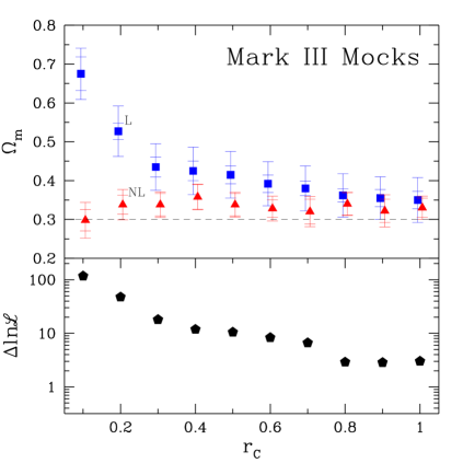
Figure 1.— Testing the method at different levels of nonlinearity. Bottom: the value of the recovered density parameter $\Omega_{m}$ as a function of the degree of linearity of the dataset, as measured by $r_{\rm c}$. The “true” value is $\Omega_{m}=0.3$. Each symbol marks the average over 10 mock M3 catalogs, and the inner error-bar marks the corresponding standard deviation. The outer error-bar is the $84\%$ likelihood uncertainty (corresponding to $\Delta{\rm ln}{\cal L}=1$), which includes cosmic variance. The squares represent the results of the likelihood analysis using the purely linear $\Lambda$CDM $P(k)$; they show a significant bias that increases with decreasing $r_{\rm c}$. The triangles represent the results of the improved analysis using a broken-$\Lambda$CDM $P(k)$; the bias is drastically reduced. Top: the corresponding mean improvement in ${\rm log}{\cal L}$ for the nonlinear analysis versus the linear analysis.

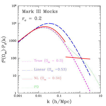
Figure 2.— Mean power spectra recovered from the M3 mock catalogs of $r_{\rm c}=0.2$. The target is the true linear $P(k)$ (marked “True”). The nonlinear correction by Peacock & Dodds (PD) is shown for comparison. The result from the linear analysis is marked “L”. The result from the nonlinear analysis with $k_{\rm b}=0.2\,(h^{-1}{\rm Mpc})^{-1}$ , marked “NL”, consists of a $\Lambda$CDM function at $k<k_{\rm b}$ and a power-law at $k>k_{\rm b}$. The $P(k)$ is in units of $\!\,(h^{-1}{\rm Mpc})^{3}$.

We have applied the likelihood analysis to each of the $10\times 10$ mock M3 catalogs. The recovered values of $\Omega_{m}$ are shown in Figure 1 as a function of the degree of linearity of the dataset, as measured by $r_{\rm c}$. The “true” target value is $\Omega_{m}=0.3$. Each symbol represents the average over the 10 mock catalogs for each value of $r_{\rm c}$. The small errorbars mark the standard deviation over these $10$ mock catalogs, and thus represent the uncertainty due to the random sampling and the random distance errors. The large errorbars are $84\%$ errors based on the likelihood analysis, namely determined by $\Delta{\rm ln}{\cal L}=1$; they thus include the effects of random distance errors and cosmic variance.

We first apply the purely linear analysis, with the linear $\Lambda$CDM power spectrum at all scales, COBE normalized, and with $\Omega_{m}$ as the only free parameter while all the other parameters are fixed at their “true” values. We see that the linear likelihood analysis systematically overestimates the value of $\Omega_{m}$. As the data become more nonlinear, the recovered value of $\Omega_{m}$ becomes higher, and the bias more significant. For example, at $r_{\rm c}=0.2$, we obtain $\Omega_{m}=0.53$, which is more than a $4\sigma$ deviation from the true value.

Next, we apply the improved procedure, allowing for a break in the $P(k)$ at $k_{\rm b}=0.2\,(h^{-1}{\rm Mpc})^{-1}$ and two additional free parameters in the nonlinear regime. As demonstrated in Figure 1, the bias is practically removed for all levels of nonlinearity. The figure also shows the corresponding improvement in ${\rm log}{\cal L}$ when the linear analysis is replaced with the nonlinear analysis. The improvement grows continuously with decreasing $r_{\rm c}$, from $\Delta{\rm ln}{\cal L}\sim 1$ at $r_{\rm c}=1$ to $\sim 120$ at $r_{\rm c}=0.1$.

Figure 2 shows the average mass-density power spectra recovered from the M3 mock catalogs of linearity $r_{\rm c}=0.2$. The true linear density $P(k)$ of the simulation, moved forward in time by linear theory, is shown for comparison. Also shown is the Peacock & Dodds (1996) nonlinear correction at large $k$. The $P(k)$ recovered by the linear likelihood analysis (L), corresponding to $\Omega_{m}=0.53$, is higher than the true $P(k)$ at $k=0.2\,(h^{-1}{\rm Mpc})^{-1}$ by a factor of $\sim 5$. The nonlinear analysis (NL), with $\Omega_{m}=0.34$ compared to the true $\Omega_{m}=0.30$, brings the $P(k)$ down much closer to the true $P(k)$.

The power-law segment at $k>k_{\rm b}$ crudely recovers the amplitude of the PD power spectrum at $k\sim 1$, but apparently not the general slope. A good agreement between the two is not obvious a priori  because the PD correction refers to the density $P(k)$, while our likelihood analysis is based on the velocity power spectrum and is still making use of the linear relation between velocity and density. We shall see below that when applied to the real data, of either M3 or SFI, the NL segment does match the PD approximation somewhat better.

The true initial power spectrum in the simulation was actually based on the $\Gamma$ functional form (e.g., Efstathiou, Bond & White 1992), which is a slightly different approximation to the $\Lambda$CDM spectrum than the one used as a prior in our likelihood analysis, Eq. (2.2). The differences between these two power spectra for the same values of $\Omega_{m}h$ are relatively small, e.g., at the level of 20% at $k=0.1$. To test the robustness of our results to these small differences in the power-spectrum shape, we also applied the same likelihood analysis to the mock catalogs using the $\Gamma$ model as prior. The free parameter in this case was $\Gamma$, which is equivalent to $\Omega_{m}$ for a fixed $h$. The normalization of $f(\Omega_{m})P(k)$ was fixed at a small wavenumber, $k=0.001(\,{\rm h^{-1}Mpc})^{-1}$, to equal the true normalization in the simulation. The results are found to be robust. For example, at a linearity of $r_{\rm c}=0.2$, the linear $\Gamma$ model yields a best fit of $\Omega_{m}=0.54$ (instead of $0.53$ when Eq. (2.2) is used, with COBE normalization), and the broken $\Gamma$ model yields $\Omega_{m}=0.36$ (instead of $0.34$).

When nonlinear effects are in action, one might worry about mode-mode coupling affecting the results in the linear regime. The unbiased estimates of the linear $P(k)$ and $\Omega_{m}$ obtained with our method when applied to the mock catalogs indicates that the modes for $k<k_{\rm b}$ are practically decoupled from modes with $k>k_{\rm b}$. We can assume that the linear modes with $k<k_{\rm b}$ are not coupled among themselves, but we do not know much about possible coupling among the nonlinear modes with $k>k_{\rm b}$. This is fine as long as we do not assign physical significance to the shape of the power spectrum recovered on these scales, beyond assuming that the overall probability distribution is well approximated by a model with a certain function playing the role of the power spectrum.

Our conclusion from the above test using the mock catalogs is that, in the presence of significant nonlinear effects in the data, the purely linear likelihood analysis might yield a biased estimate of $P(k)$ and $\Omega_{m}$. The broken-$P(k)$ analysis successfully eliminates the dependence of the results on the nonlinear effects and practically corrects the bias in the results.

4. RESULTS

4.1. Broken $\Lambda$CDM: the Value of $\Omega_{m}$

We now apply the improved likelihood analysis to the real data of M3 and SFI. Similar to the tests with the mock data, our $\Lambda$CDM model is restricted to a flat universe with $h=0.65$, $\Omega_{b}h^{2}=0.02$ and $n=1$, leaving only one cosmological parameter free to be determined by the maximum likelihood analysis, namely $\Omega_{m}$. Note that contrary to the situation in the mock catalogs we now do not know a priori  that the $\Lambda$CDM model is the right one or that the values of the fixed parameters are the accurate ones. The purely linear analysis yields $\Omega_{m}=0.56\pm 0.04$ and $\Omega_{m}=0.51\pm 0.05$ for M3 and SFI respectively ($90\%$ errors), consistent with Z97 and F99 when $h$ and $n$ are fixed at the values quoted above. Based on the test using mock catalogs, we now suspect that these might be overestimates.

Figure 3.— The recovered power spectra from the real data of M3 (left) and SFI (right). The $P(k)$ yielded by the purely linear analysis is marked “L”, while the nonlinear analysis, with a break at $k=0.2\,(h^{-1}{\rm Mpc})^{-1}$, is marked “NL”. Also shown for comparison is an extrapolation of the linear part of the recovered $P(k)$ into the nonlinear regime by the PD approximation. The $P(k)$ is in units of $\!\,(h^{-1}{\rm Mpc})^{3}$.

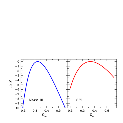
Figure 4.— Likelihood function for the values of $\Omega_{m}$ due to the nonlinear analysis with $k_{\rm b}=0.2\,(h^{-1}{\rm Mpc})^{-1}$, from the real data of M3 (left) and SFI (right).

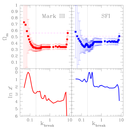
Figure 5.— Robustness to the break scale. The results of the nonlinear analysis with the broken-$\Lambda$CDMpower spectrum, for the real data, as a function of the break length $k_{\rm b}$ in units of $\!\,(h^{-1}{\rm Mpc})^{-1}$. The errors are $84\%$ from the likelihood function. Bottom: the recovered value of $\Omega_{m}$. Top: the corresponding likelihood. Left: M3. Right: SFI.

Figure 3 shows the maximum-likelihood power spectra as derived from the two catalogs of real data. The linear analysis yields a high amplitude, corresponding to a high value of $k_{\rm peak}$ where $P(k)$ is at maximum, and the corresponding high value of $\Omega_{m}$.

The nonlinear analysis with a break at $k_{\rm b}=0.2\,(h^{-1}{\rm Mpc})^{-1}$ yields a shift of $k_{\rm peak}$ towards lower $k$ values, associated with a lower value of $\Omega_{m}$, and a corresponding lower amplitude for $P(k)$ in much of the linear regime. The new values are $\Omega_{m}=0.32\pm 0.06$ for M3 and $\Omega_{m}=0.37\pm 0.09$ for SFI.

The corresponding best-fit values of $\sigma_{8}\Omega_{m}^{0.6}$ are $0.49\pm 0.06$ and $0.63\pm 0.08$ for M3 and SFI respectively. These values are consistent with the estimates from cluster abundance (e.g., Eke et al. 1998).

The change caused in the value of $\Omega_{m}$ due to the nonlinear correction is similar to the corresponding change in the mock catalogs of M3 at a relatively high degree of nonlinearity, $r_{\rm c}\simeq 0.2$ in Figure 1.

The best-fit power-law segments in the nonlinear regime are $145k^{-0.8}$ for M3 and $155k^{-1.4}$ for SFI (where $k$ is in units of $\!\,(h^{-1}{\rm Mpc})^{-1}$, and $P(k)$ in units of $\!\,(h^{-1}{\rm Mpc})^{3}$. The power-law segments roughly coincide with the linear $\Lambda$CDM segments at $k_{\rm b}$, indicating that this broken power spectrum is a sensible approximation to the actual shape of the $P(k)$. Interestingly, the best-fit power laws match quite closely the PD nonlinear corrections for the density $P(k)$. This match should not be taken as a very meaningful estimate of the actual shape of the power spectrum in the nonlinear regime. Our nonlinear segment results from applying a procedure that is still based on the linear gravitational instability relation between velocity and density to a phenomenon that is fully nonlinear. We have no immediate reason to expect the PD formalism to extend to peculiar velocities so straightforwardly. We therefore take this match only as a crude guideline to encourage further investigations into the behaviour of the velocity power spectrum (and the likelihood function) in the mildly nonlinear regime.

As expected, the nonlinear correction for the M3 catalog is larger than for the SFI data, because the former has more galaxies nearby and therefore a larger number of close pairs with small errors. The M3 $P(k)$, which was somewhat higher than SFI in the linear analysis, becomes somewhat lower than SFI as a result of the nonlinear analysis, but the two catalogs basically yield consistent results. The likelihood improvement for M3 is very significant, $\Delta{\rm ln}{\cal L}\simeq 22$, while for SFI it is moderately significant, $\Delta{\rm ln}{\cal L}\sim 2.8$.

Figure 4 shows the likelihood as a function of $\Omega_{m}$ for each of the two datasets, where for each value of $\Omega_{m}$, the power-law parameters in the nonlinear regime obtain their most likely values. The maximum is narrower for M3 than for SFI. When, instead, we marginalize over the two power-law parameters in the nonlinear regime, the obtained best $\Omega_{m}$ remains the same (to within $0.01$) and the likelihood function becomes wider by $4\%$.

Although we may expect the position of the break in the power spectrum, $k_{\rm b}$, to be in the vicinity of $k\sim 0.2$ (e.g., from the PD approximation), we should check the robustness of our results to the actual choice of $k_{\rm b}$. Figure 5 shows the derived values of $\Omega_{m}$ and the corresponding likelihood as a function of the value of $k_{\rm b}$. We find that the results are quite insensitive to the choice of $k_{\rm b}$ over a wide range. At $k_{\rm b}$ values much smaller than $0.1$, corresponding to large separations between pairs of objects and thus involving mostly distant objects of large errors, there are insufficient data to constrain the power spectrum, and therefore the errors become big and the results quite meaningless. At very large values of $k_{\rm b}$, the analysis is expected to recover the results of the old linear analysis with no break. It indeed does so, but only when $k_{\rm b}$ approaches the artificial cutoff applied to $P(k)$ arbitrarily at $k_{\rm max}=8\,(h^{-1}{\rm Mpc})^{-1}$ for the purpose of finite numerical integration. It seems that any little freedom allowed in the model beyond the strict linear power spectrum is enough for correcting the bias associated with the linear analysis.

As mentioned earlier, an alternative way to incorporate nonlinear effects is by adding to the linear velocity correlation model a free parameter of uncorrelated velocity dispersion at zero lag, $\sigma_{\rm v}$. When this nonlinear correction is applied by itself to the M3 data, the best value of $\Omega_{m}$ becomes $0.38$ (instead of 0.56 in the linear analysis) with $\sigma_{\rm v}=250\,{\rm km\,s^{-1}}$.

We then apply to M3 the two different nonlinear corrections together, i.e., a break in the power spectrum at $k=0.2$ as well as a free velocity dispersion term. Figure 6 shows a map of the resulting likelihood in the $\Omega_{m}$-$\sigma_{\rm v}$ parameter plane. The best-fit value of $\sigma_{\rm v}$ is close to zero, indicating that the two nonlinear corrections are practically redundant.

4.2. Deviations from $\Lambda$CDM

Encouraged by the success of breaking the power spectrum into two detached segments, we now push the idea further, and divide the power spectrum into 4 detached segments. This allows a more general shape for $P(k)$, less dependent of a priori  assumptions about a physical model such as $\Lambda$CDM. By doing so we may detect clues for deviations from the “standard” $P(k)$ shape, but in this case we clearly give up the attempt to determine cosmological parameters.

Our 4-band model for $P(k)$ consists of the following segments:

1. COBE-normalized $\Lambda$CDM in the extreme linear regime, $k\leq 0.02$, with $\Omega_{m}$ fixed at the most likely value from the nonlinear analysis.

2. A free constant amplitude in the interval $0.02<k\leq 0.07$, at the vicinity of $k_{\rm peak}$.

3. An independent free constant amplitude in the interval $0.07<k\leq 0.2$, just short of the transition between the linear and nonlinear regimes.

4. A power law with two free parameters (as before) in the nonlinear regime, $k>0.2$.

Figure 7 shows the recovered 4-band $P(k)$ from the real data of M3 and SFI, in comparison with the $\Lambda$CDM results of the linear and nonlinear analysis discussed above. The most likely parameters of the three meaningful segments ($k>0.02$) are $(9750,\,370,\,160k^{-0.95})$ for M3 and $(7450,\,1000,\,160k^{-1.40})$ for SFI, where the amplitudes are in unites of $\!\,(h^{-1}{\rm Mpc})^{3}$ and $k$ is in units of $\!\,(h^{-1}{\rm Mpc})^{-1}$. The errors are shown in the figure.

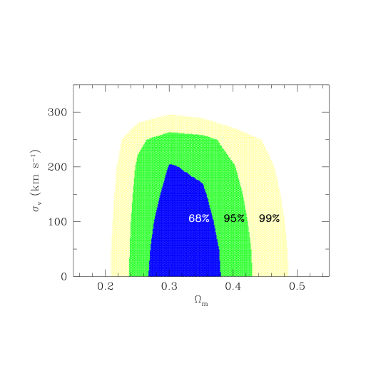
Figure 6.— Robustness to different nonlinear corrections. The likelihood, for the real M3 data, when allowing both a break at $k=0.2$ and a velocity-dispersion term, as a function of the free parameters $\Omega_{m}$ and $\sigma_{\rm v}$. The contours correspond to 68%, 95.4% and 99.73% in the two-parameter plane.

Figure 7.— The 4-band power spectrum for the M3 (left) and SFI (right) data, compared to the best-fit $\Lambda$CDM power spectra, linear (L) and nonlinear with a break (NL).

The nonlinear segment, not surprisingly, practically recovers the results of the broken-$\Lambda$CDM analysis. The most linear segment can be fixed almost arbitrarily without affecting the results in the two inner bands. This is not surprising either since we cannot expect our current data to contstrain the power spectrum on these very large scales.

The second segment in the linear regime, $(0.02,\,0.07)$, tends to lie above the peak obtained in the broken-$\Lambda$CDM analysis, while the third linear interval, $(0.07,\,0.2)$, in the “blue” side of the peak, shows a low amplitude. We thus see a “wiggle” about the linear portion of the broken-$\Lambda$CDM best fit, which is detected independently in the two data sets. The features in the linear regime contribute only a marginal improvement to the overall likelihood, which is still dominated by the nonlinear segment. The significances of the deviations, both the excessive peak and the low dip, are slightly above 1$\sigma$ each. Our finding should therefore be considered as a marginal hint only; it could be just a fluke due to the distance errors and cosmic variance. But it is still an intriguing feature, especially since it appears consistently in our two samples.

The marginal deviation from the broken-$\Lambda$CDM $P(k)$ thus consists of a wiggle, with a power excess near the peak, $k\sim 0.05$, and a deficiency at $k\sim 0.1$. The missing power is reminiscent of the indications for “cold flow” in the galaxy peculiar velocity field in the local cosmological neighborhood. While the streaming motions on scales of a few tens of megaparsecs are on the order of several hundreds of kilometers per second, the dispersion velocity of field galaxies is only on the order of $\sim 200\,{\rm km\,s^{-1}}$, indicating a high Mach number on comparable scales (e.g., Suto, Cen & Ostriker 1992; Chiu, Ostriker & Strauss 1998; Dekel 2000).

A hint for a similar wiggly feature has been detected in the density $P(k)$ as derived by some of the researchers from the distribution of galaxies (Baugh & Gaztañaga 1998; Landy et al. 1996) and clusters (Einasto et al. 1997; Suhhonenko & Gramann 1999). Most recently, there are indications for such a wiggle in the preliminary $P(k)$ derived from part of the 2dF redshift survey (private communication with the 2dF team).

Most interestingly, the scale of the missing power in our local $P(k)$ from velocities roughly coincides with the scale of the second peak in the angular spectrum of the CMB. Preliminary balloon measurements (Boomerang, de Bernardis et al. 2000; Maxima, Hanany et al. 2000) indicate that this peak is somewhat lower than expected by the common CDM models. This may be a reflection of the same phenomena which we detect here as “cold flow” in the peculiar velocity data.

The scale of the wiggly feature roughly coincides with the most obvious physical scale in cosmology — the size of the cosmological horizon at the time of transition from radiation to matter dominance, or slightly later, at the epoch of plasma recombination and radiation-matter decoupling. A wiggle on these scales can be produced by an excess of either baryons or massive neutrinos in the cosmological mass budget. But the excess required to produce a significant wiggle seems to violate upper limits from other data; the density of baryons is limited by He+D abundances via the theory of Big-Bang nucleosynthesis (Tytler et al. 2000), and the density of neutrinos is constrained by large-scale structure (e.g., Ma 1999; Gawiser 2000).

5. PRINCIPAL COMPONENT ANALYSIS

The linear $\Lambda$CDM analysis of both the M3 and SFI data (Z97; F99) revealed a warning signal concerning the GOF, which we termed “the two-halves problem”. When the linear analysis is applied separately to two halves of the data, separated either by the median distance or by line-width (which is correlated with the distance), the results are somewhat different. The distant data prefer a lower-amplitude power spectrum, associated with a lower value of $\Omega_{m}$. The mock catalogs (tested with the true correlation matrix) have not revealed a similar problem, indicating that it is caused by inadequacies of the correlation matrix compared with the real data. These shortcomings may be associated with the assumed theoretical model, either the shape of the $P(k)$ or the Gaussian nature of the fluctuations, or with the error model, either its Gaussianity or its radial dependence. These worries motivate an attempt to evaluate the GOF in our linear and nonlinear analyses. In particular, we wish to see to what extent the revised $P(k)$ in the nonlinear regime may resolve the two-halves problem.

Assume a data vector ${\bf d}$, which is a random realization of an $n$-dimensional multivariate Gaussian distribution, with the correlation matrix $C=\langle{\bf d}{\bf d}^{\dagger}\rangle$. A global GOF could be evaluated using the $\chi^{2}$ statistic, $\chi^{2}={\bf d}^{\dagger}C^{-1}{\bf d}=Tr(C^{-1}D)$, where $D\equiv{\bf d}{\bf d}^{\dagger}$. If $C$ is the true correlation matrix, then this quantity should obey a $\chi^{2}$ distribution with $n$ degrees of freedom, as indeed is the case for all the analyses we performed. But this single number cannot capture all the particulars of the fitting process.

A Principal-Component Analysis, in which the data are represented in terms of the eigenvector basis of the (assumed) correlation matrix, is a powerful tool for our purposes in several different ways. Our original motivation for applying a PCA (following Vogeley & Szalay 1996; Tegmark, Taylor & Heavens 1997) was to allow optimal compression of the data into the modes that are most important for estimating the parameters we wish to evaluate, with the aim to reduce the computational cost associated with inverting huge correlation matrices, and to improve the results given an inaccurate correlation matrix. In the current paper, we use a PCA for two other purposes. First, we present a novel approach of using the PCA modes for identifying certain gross features of the data and model via the correlation matrix. Second, we extend a method first used by Hoffman & Zaroubi (2000) for evaluating GOF in fine detail and for trying to resolve the two-halves problem.

5.1. Modes of $S+N$ versus $S/N$

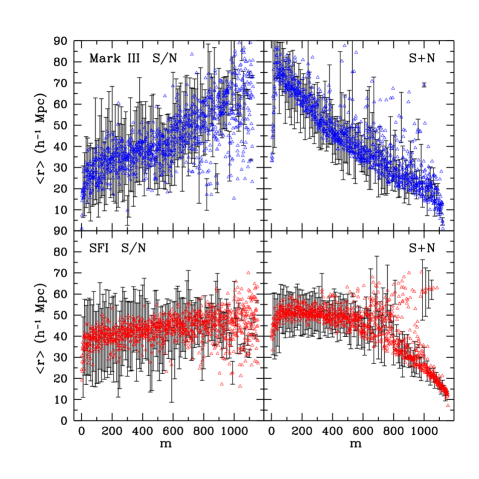
Figure 8.— Average distances associated with the eigenmodes of the correlation matrix of the linear $\Lambda$CDM model. The eigenmodes are ranked by decreasing eigenvalue amplitude. (low $m$ — high eigenvalue). The standard deviation is shown for every tenth mode. Left: $S/N$ modes. Right: $S+N$ modes. Top: M3 data. Bottom: SFI data.

The standard PCA is as follows. A general coordinate transfromation of the data ${\bf d}$ defines a new set of $m$ random variables $\tilde{{\bf d}}=\Psi{\bf d}$, where $\Psi$ is an $m\times n$ matrix, which we assume to be of full rank. It is then clear that the distribution of the new variables is still Gaussian, with a correlation matrix $\widetilde{C}=\langle\widetilde{{\bf d}}\widetilde{{\bf d}}^{\dagger}\rangle=\Psi C\Psi^{\dagger}$. The likelihood analysis can be performed in terms of these new “data” points. If we keep all the original information, i.e., if $\Psi$ is invertible, the likelihood analysis is not affected because then $Tr(\tilde{C}^{-1}\tilde{D})=Tr(C^{-1}D)$. Since the correlation matrix is symmetric and positive definite, we can, without loss of generality, pick the matrix $\Psi$ such that $\tilde{C}$ is diagonal. Then the rows $\tilde{d}_{i}$ of $\Psi$ are the eigenvectors of the correlation matrix, or its principal components, and the diagonal terms $\lambda_{i}$ of $\tilde{C}$ are the corresponding eigenvalues, In statistical terms this means that the new variables are expected to be uncorrelated. The validity of this independence of variables is a measure of GOF. We thus use the $\chi^{2}$ statistic to test the hypothesis that $\tilde{d}_{i}/\sqrt{\lambda_{i}}$ are uncorrelated unit Gaussian random variables. If this test uncovers systematic effects, it may become possible to associate them with certain features of the data and model via a further investigation of the eigenmodes.

The eigenmodes are ordered by the amplitude of their eigenvalues, from large to small, and the high-eigenvalue modes are assigned a higher signifcance, because the confidence levels in the recovered parameters of a maximum-likelihood analysis inversly correlate with the squares of the eigenvalues of the modes used (Tegmark, Taylor & Heavens 1997). Furtheremore, perturbation analysis implies that small-eigenvalue modes are more sensitive to perturbations in the correlation matrix, implying that the mode-by-mode statistical tests may not be reliable for small-eigenvalue modes. Since our correlation matrix is expected to be only an approximation to the true correlation matrix, it would be advantageous, in general, to avoid small-eigenvalue modes, and rely on the high-eigenvalue ones.

A straightforward application of PCA is with the original correlation matrix of Eq. (3), which is a sum of signal and noise: $C=S+N$. In this case, the large eigenvalues may correspond either to large signal, or large noise, or both. Another possibility, which we term $S/N$, is to first perform a “whitening” transformation, $\hat{{\bf d}}=N^{-\frac{1}{2}}{\bf d}$ (Vogeley & Szalay 1996). In the case of a diagonal noise matrix $N$, this transformation amounts to normalizing the data in terms of the expected noise. The new correlation matrix is $\hat{C}=N^{-\frac{1}{2}}SN^{-\frac{1}{2}}+I$, where $I$ is the identity matrix. The eigenvalues of $\hat{C}$ are the signal-to-noise ratios of the corresponding principal modes.

5.2. Correlation Between Mode and Distance

The eigenmodes can help us identify certain features of the data and models. In particular, the signal part involves the geometry of sampling and the prior model, and the noise part involves the distance error estimates. A useful diagnostic statistic to assign with each eigenmode is the distance from the Local Group. For eigenvector $v$, the average distance is

$$\langle r\rangle_{v}=\sum_{g}|v(g)|^{2}r(g)\,,$$ (10)

where the sum is over the sample of galaxies, $r(g)$ is the distance of galaxy $g$, and $v(g)$ defines the vector $v$ in the basis $g$. This is a weighted average of the galaxy distances. The variance $\left\langle(r-\langle r\rangle_{v})^{2}\right\rangle_{v}$ is defined in analogy. If the standard deviation is small compared to the average distance, one can conclude that most of the information associated with this mode comes from galaxies within a certain distance range.

The distance associated with a mode provides important information about the mode: distant modes are typically noisier than nearby ones because the distance error is proportional to distance. The correlation between modes and distance could also help us understand the two-halves problem. In the following mode-by-mode analysis, we use this correlation to interpret a correlation with mode number as a correlation with distance.

Figure 8 shows the average distance for each mode, for the linear $\Lambda$CDM model and either the M3 or SFI data. We see that the $S/N$ modes are correlated with distance, such that the high-eigenvalue modes, which are robust and of high signal-to-noise ratio, are typically associated with nearby data, which are of relatively small errors. On the other hand, these nearby modes tend to involve close galaxy pairs, and are therefore more subject to nonlinear effects, which makes the nonlinear correction a must. The correlation is strong for M3, and weaker for SFI.

The $S+N$ modes show a somewhat stronger correlation in the opposite sense, in which the high-eigenvalue modes, except for the first few, are typically associated with large distances and therefore noisy data. This means that most of the $S+N$ modes are dominated by the noise rather than the signal. This situation is unfortunate for the $S+N$ PCA; for example, it does not allow a sensible truncation by $S+N$ modes. But it should allow a more sensitive measure of GOF, refering in particular to the error model. Again, the correlation is stronger for M3 than for SFI.

5.3. Goodness of Fit Mode by Mode

After PCA, assuming that we know the true correlation matrix, the variables $\widetilde{{\bf d}}$ are expected to be uncorrelated, and we expect $\chi^{2}_{i}=\tilde{d}_{i}^{2}/\lambda_{i}$ to be about unity for each and every mode separately. The validity of this behavior mode by mode provides an improved and finer test of GOF in two ways. First, it tests whether the eigenmodes of the prior correlation matrix are really uncorrelated, with the variance determined by the eigenvalues. Then, in the case of a poor fit for a certain mode, it can guide us to the source of the poor fit via the properties associated with that mode.

One statistic we use, for each mode number $m$, is the cumulative $\chi^{2}$ per degree of freedom, $\sum^{m}_{i=1}\chi_{i}^{2}/m$, in which the sum starts from the high-eigenvalue modes and ends at mode $m$. In the case of independet modes, the expected value is unity, and the expected standard deviation is about $\sqrt{2/m}$ (the normalized standard deviation of a $\chi^{2}$ distribution with m degrees of freedom).

A second set of more localized statistics is the differential estimates, obtained by averaging the $\chi^{2}$ values over intervals of mode numbers of length $s$ namely, using $\sum_{i=m-s+1}^{m}\chi_{i}^{2}/s$ for various values of $m$. If the correlation matrix was exact, these would be independent (assuming the intervals are disjoint) and follow a $\chi^{2}$ distribution with $s$ degrees of freedom. In particular, the expectation value would be unity with a standard deviation $\simeq\sqrt{2/s}$. We choose $s=50$, which is large enough for good statistics and small enough with respect to the total $n$ for the purpose of tracing systematic effects.

Figure 9 shows the cumulative $\chi^{2}$ statistic as a function of $m$ for the linear $\Lambda$CDM analysis and for the nonlinear broken-$\Lambda$CDM analysis. Figure 10 shows the corresponding differential $\chi^{2}$ statistic.

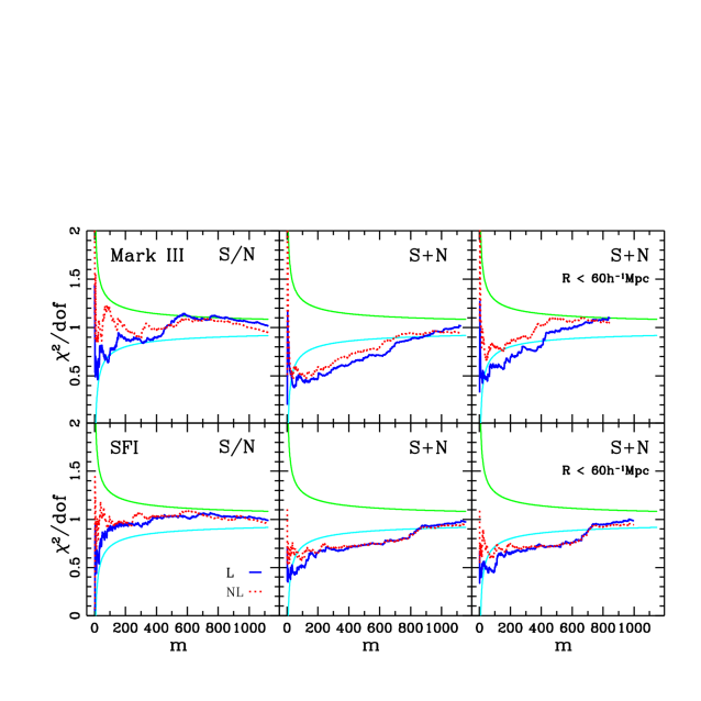
Figure 9.— Cummulative $\chi^{2}$ per degree of freedom as a function of mode number. The heavy solid curve is for the linear $\Lambda$CDM model, and the dotted curve is for the broken-$\Lambda$CDM power spectrum. The two solid lines mark the expected $2\sigma$ deviations. Left: $S/N$ modes. Middle: $S+N$ modes. Right: $S+N$ modes, for the data at $r<60\,{\rm h^{-1}Mpc}$ only. Top: M3 data. Bottom: SFI data.

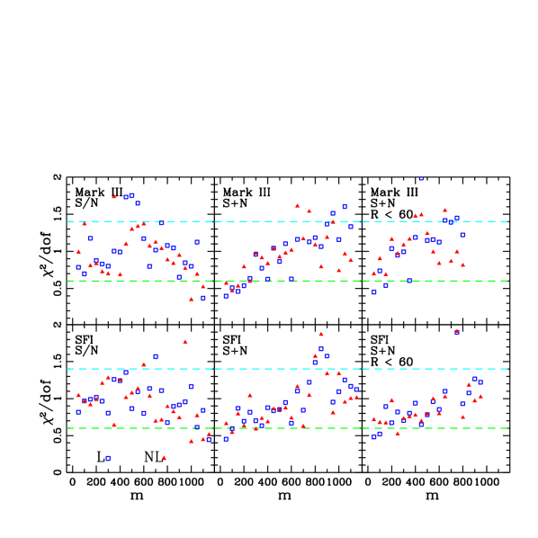
Figure 10.— Differential $\chi^{2}$ per degree of freedom as a function of mode number. The open squares are for the linear $\Lambda$CDM model, and the filled triangles are for the broken-$\Lambda$CDM power spectrum. The two dashed lines mark the expected $2\sigma$ deviations. Left: $S/N$ modes. Middle: $S+N$ modes. Right: $S+N$ modes, for the data at $r<60\,{\rm h^{-1}Mpc}$ only. Top: M3 data. Bottom: SFI data.

For the $S/N$ modes of M3, the GOF of the linear model is marginal, in the sense that the typical deviations in the cumulative statistic are at the $2\sigma$ level. The low-$m$ modes, except for the very first ones, typically have low $\chi^{2}/dof$ values, while the large-$m$ modes have high values. This systematic behavior with $m$ can be translated to a systematic correlation with distance via the correlation between distance and mode (Figure 8). It is therefore a reminiscence of the two-halves problem.

Can we use the PCA to distinguish between an inadequate model of $P(k)$ and a problem in the error model? We see in Figure 9 that the broken-$\Lambda$CDM model clearly improves the GOF as far as the $S/N$ modes of M3 are concerned. With this model, the cumulative $\chi^{2}/dof$ lies well inside the $2\sigma$ contours for all the modes, with no apparent systematic dependence on $m$. It implies that the broken-$\Lambda$CDM $P(k)$ is a more appropriate model for the data. Based on the $S/N$ modes, there is no indication that the error model may be inadequate.

When we analyze the $S+N$ modes in a similar way in Figure 9, the linear model, for both data sets, shows a more severe deviation of $\chi^{2}/dof$ from unity, at the $4-5\sigma$ level, and a similar systematic dependence on $m$. This trend is also apparent in Figure 10 (middle panels). The two-halves problem is very obvious here, with the more distant data, corresponding to larger eigenvalues and larger noise, favoring a smaller amplitude for the power spectrum than the nearby data. In this case, the use of the better, broken-$\Lambda$CDM model makes only a small improvement which does not resolve the problem. This is a clear indication that something may be wrong in the error model as well.

We then recall that the low-$m$ $S+N$ modes are associated with large distances, where the errors are large and are known to a lesser accuracy. Guided by Figure 8, we try a poor-man compression of the data by eliminating from the analysis all the data points that lie at an inferred distance greater than $60\,{\rm h^{-1}Mpc}$. This leaves us with $843$ out of the $1124$ (grouped) data points of M3, and $996$ out of the $1156$ galaxies of SFI. This truncation makes only a negligible change in the the best-fit value of $\Omega_{m}$ (an increase of less than $3\%$, both for M3 and SFI), and it causes only a minor widening of the likelihood contours. In the case of M3, we see in Figure 9 that the $S+N$ modes of the linear model and truncated data show an improved GOF compared to the case of the whole data, but the $\chi^{2}/dof$ still show $\sim 3\sigma$ deviations from unity and a systematic dependence on $m$. However, the $S+N$ modes of the broken-$\Lambda$CDM model and truncated M3 data now do lie within the $2\sigma$ contours. The systematic trend with $m$ is still apparent, indicating that the correlation matrix is still not perfect; either the error model is only an approximation even for the truncated data, or the broken-$\Lambda$CDM $P(k)$ is not yet a perfect model (as seen in §4.2), or the signal and/or the noise are not exactly Gaussian.

In the case of SFI, while the $S/N$ modes look very adequate with both models, for the $S+N$ cumulative statistic the improvements due to the nonlinear correction and the elimination of large-distance galaxies are apparently not enough for an acceptable GOF. According to the differential statistic, the nonlinear correction and truncation do bring each of the first few bins into their $2\sigma$ range, but the fact that many of these bins are each not much above the $-2\sigma$ line makes the cumulative statistic lie outside its $2\sigma$ range. Since the large-eigenvalue $S+N$ modes, which dominate the cumulative statistic, are dominated by noise, the limited GOF is likely to point at further shortcomings of the error model for SFI.

6. CONCLUSION

A likelihood analysis is supposed to recover unbiased values for the free parameters of a model provided that the prior theoretical model and the error model allow accurate description of the data. We addressed here tools to recover the parameters given incomplete knowledge of these models.

Using mock catalogs based on high-resolution simulations, we realized that the likelihood analysis of peculiar-velocity data, based on the linear $\Lambda$CDM power spectrum, is driven by the nonlinear part of the spectrum which is not modeled accurately, and might therefore yield biased results. For example, in the linear analysis of the M3 mock data, the obtained amplitude of $P(k)\Omega_{m}^{1.2}$ is overestimated, corresponding to a positive bias in the cosmological density parameter $\Omega_{m}$ by $\sim 35\%$.

A broken-$\Lambda$CDM power spectrum, in which the $k>k_{\rm b}$ segment of the power spectrum is replaced by a more flexible two-parameter power law, allows a better, independent fit in the nonlinear regime. It then frees the linear part of the spectrum from nonlinear effects, and yields unbiased results for $\Omega_{m}$. The results are robust to the specific choice of $k_{\rm b}$; we choose $k_{\rm b}=0.2\,(h^{-1}{\rm Mpc})^{-1}$, which is where the nonlinear density $P(k)$ is expected to start deviating from the linear $P(k)$ by the PD approximation. The results are also robust to the exact way by which the nonlinear effects are incorporated. When we add a zero-lag velocity dispersion term to the correlation function, either replacing the break in the power spectrum or in addition to it, the results are similar.

We note that these procedures do not mean to tell us much about the actual power spectrum in the nonlinear regime, as our improved analysis in the nonlinear regime is still based on the linear relation betweem velocity and density. For an improvement in this direction, one should come up with a physically motivated functional form that accounts for mildly nonlinear corrections to the linear velocity power spectrum, in analogy to the PD correction to the density $P(k)$. Nevertheless, as demonstrated by the tests based on mock catalogs and by the robustness to the actual nonlinear correction applied, our current procedures are reliable for eliminating the biases in the linear regime.

When applied to the real data of M3 or SFI peculiar velocities, assuming a flat $\Lambda$CDM model with $n=1$ and $h=0.65$, the improved analysis yields best-fits of $\Omega_{m}=0.32\pm 0.06$ and $0.37\pm 0.09$ respectively, corresponding to $\sigma_{8}\Omega_{m}^{0.6}\approx 0.49\pm 0.06$ and $0.63\pm 0.08$ respectively. These values are in good agreement with most constraints from other data, including CMB anisotropies and cluster abundance (e.g., Bahcall et al. 1999). It is important to stress that the estimates of the cosmological parameters reported here are valid under the assumption that the power spectrum in the liner regime is drawn from the flat $\Lambda$CDM cosmolgical model with $\Omega_{m}$ as a free parameter. In our current nonlinear analysis of the data inside $60\,{\rm h^{-1}Mpc}$, the maximum-likelihood solution based on the $\Lambda$CDM power spectrum indeed has an acceptable goodness-of-fit, making our estimate of $\Omega_{m}$ self-consistent and meaningful. Although we conclude below that our error model is not accurate for M3 beyond $60\,{\rm h^{-1}Mpc}$ and for SFI, the obtained value of $\Omega_{m}$ is insensitive to the exclusion of the noisy data beyond $60\,{\rm h^{-1}Mpc}$ and to other changes in the error model.

By allowing a more general shape for the power spectrum, with 4 detached segments, we detect a marginal indication for a deviation from the $\Lambda$CDM power spectrum. The possible deviation is characterized by a wiggle, with an enhanced amplitude near $k_{\rm peak}\sim 0.05$ and a depletion near $k\sim 0.1\,(h^{-1}{\rm Mpc})^{-1}$. The study of possible deviations from the $\Lambda$CDM model is done at the expense of the attempt to estimate $\Omega_{m}$, which requires a power-spectrum shape based on a physical cosmological model. Nevertheless, we learn from the 4-band analysis that the relatively low $\Omega_{m}$ estimate in the broken-$\Lambda$CDM analysis is driven by the low amplitude of the power spectrum near $k\sim 0.1\,(h^{-1}{\rm Mpc})^{-1}$.

The indicated “cold flow” on a scale of a few tens of megaparsecs is reminiscent of similar indications from the power spectrum of galaxies and clusters in redshift surveys (§4.2). Most recent is the wiggle seen in the preliminary power spectrum derived from the 2dF redshift survey. The local cold flow may be related to the second peak in the CMB angular power spectrum on a similar scale. The wiggly feature in the power spectrum may be interpreted as a possible indication of a deviation from the standard cosmological mass mixture, e.g., a higher baryonic content than indicated by the Deuterium abundance and Big-Bang nucleosynthesis, or a non-negligible contribution from hot dark-matter in the form of massive neutrinos. However, the possibility that this feature is a statistical fluke due to cosmic variance in the context of the $\Lambda$CDM model cannot be ruled out yet.

A principal component analysis, either in $S/N$ or $S+N$ modes, allows a fine test of goodness of fit, by applying a $\chi^{2}$ test mode by mode. It shows that the broken-$\Lambda$CDM model is a better fit to the data than the purely linear $\Lambda$CDM model. For M3, using the “whitened” $S/N$ modes, the nonlinear correction is enough to eliminate the “two-halves” problem that troubled the linear analysis. This indicates that the $\Lambda$CDM model is a good model for the signal. When the $S+N$ modes are analyzed, the correction to the theoretical model is helpful but not enough for an acceptable GOF. When the M3 data is further truncated at $60\,{\rm h^{-1}Mpc}$, eliminating distant galaxies for which the errors are large and the error model is inaccurate, the GOF becomes acceptable. This strengthens the reliability of our parameter estimates based on the assumed $\Lambda$CDM model in the linear regime. Future investigations should refine the error model at large distances, in order to possibly reduce the cosmic variance in our estimates. For SFI, the $S/N$ modes seem adequate, confirming again the suitability of the $\Lambda$CDM model in the linear regime, but the $S+N$ PCA indicates that the errors in this catalog are still more complex than assumed.

The PCA is a powerful tool for addressing interesting properties of the data and its relation to the best-fit theoretical and error models. In particular, we associated each mode with a geometric property — the mean distance and the variance about it — and thus learned about the correlation between mode eigenvalues and distance errors. This was useful in the study of GOF and in truncating the data to deal with inaccuracies in the error model. The PCA will be extremely useful when one tries to compress the data while keeping the optimal part for determining a specific desired parameter. This compression may be mandatory for computational reasons when the body of data is excessively large. Since the model is expected to be incomplete, either in terms of the theoretical assumptions or the errors, a proper compression of the data may in fact improve the results. Such data compression using PCA in the context of the analysis of cosmic flows is in progress.

Our conclusions can be summarized at three levels, as follows. First, if one is willing to assume  the “standard” $\Lambda$CDM power-spectrum shape in the linear regime, then the nonlinear corrections yield an unbiased value of $\Omega_{m}\sim 0.35$, consistently from the two data sets. The GOF is acceptable for this nonlinear analysis and the cosmological model and errors assumed, once the M3 data inside $60\,{\rm h^{-1}Mpc}$ are considered (and the value of $\Omega_{m}$ is insensitive to the inclusion of the other, noisy data). This makes the parameter estimation self-consistent and meaningful, and this is our strongest result. Second, once we alleviate the requirement of a physically motivated power spectrum and its dependence on cosmological parameters, we detect a marginal indication for a wiggle about the $\Lambda$CDM power spectrum in the linear regime. This is a marginal detection, which does not ivalidate the suitability of the $\Lambda$CDM model for the cosmological parameter estimation performed above. The hint for a wiggle is still intriguing because it repeats in the two data sets, it seems to coincide with similar clues from other data, and it may have interesting theoretical implications on the nature of dark matter and the initial fluctuations. Third, we learn from our newly developed PCA analysis that in order to possibly impprove the statistics one should refine the error model for the most distant galaxies in M3, and for a larger fraction of the galaxies in SFI. But our parameter estimates and the marginal detection of a wiggle are driven by the part of the data for which the error model yields an acceptable goodness of fit.

References

- (1) Bahcall, N., Ostriker, J., Perlmutter, S., & Steinhardt, P. 1999, Science, 284, 1481
- (2) Bardeen, J. M., Bond, J. R., Kaiser, N., & Szalay, A. S. 1986, ApJ, 304, 15
- (3) Baugh, C. M., & Gaztañaga, E., 1998, in Proceedings: Evolution of Large Scale Structure (astro-ph/9810184)
- (4) Bernardeau, F., Juszkiewicz, R., Dekel, A., & Bouchet, F., 1995, MNRAS, 274, 20
- (5) Blanton, M., Cen, R., Ostriker, J. P., & Strauss, M. 1999, ApJ, 522, 590
- (6) Branchini, E., et al. 2000, submitted
- (7) Bridle, S., Zehavi, I., Dekel, A., Lahav, O., Hobson, M. P., & Lasenby, A. N. 2001, MNRAS, 321, 333
- (8) Bunn, E. F., & White, M. 1997, ApJ, 480, 6
- (9) Burles, S., Nollett, K. M., Truran, J. N., & Turner, M. S. 1999 Phys. Rev. Lett., 82, 4176
- (10) Chiu, W.A., Ostriker, J.P., & Strauss, M.A. 1998, ApJ, 494, 479
- (11) da Costa, L. N., Freudling, W., Wegner, G., Giovanelli, R., Haynes, M. P., & Salzer, J. J. 1996, ApJ, 468, L5
- (12) da Costa, L. N., Nusser, A., Freudling, W., Giovanelli, R., Haynes, M. P., Salzer, J. J., & Wegner, G. 1998, ApJ, 299, 425
- (13) Davis, M., Nusser, A., & Willick, J. A. 1996, ApJ, 473, 22
- (14) de Bernardis, P., et al. 2000, Nature, 404, 955
- (15) Dekel, A. 2000, in Cosmic Flows: Towards an Understanding of Large-Scale Structure, eds. S. Courteau, M.A. Strauss, & J.A. Willick, ASP Conf. Series, p. 420 (astro-ph/9911501)
- (16) Dekel, A., Eldar, A., Kolatt, T., Yahil, A., Willick, J. A., Faber, S. M., Courteau, S., Burstein, D. 1999, ApJ, 522, 1
- (17) Dekel, A. & Rees, M. J. 1994, ApJ, 422, L1
- (18) Dekel, A., & Lahav, O. 1999, ApJ, 520, 24
- (19) Einasto, J., et al. 1997, Nature, 385, 139
- (20) Efstathiou, G., Bond, J. R., & White, S. D. M. 1992, MNRAS, 258, 1p
- (21) Eke, V. R., Cole, S., Frenk, C. S. & Henry, J. P. 1998, MNRAS, 298, 1145
- (22) Fisher, K. B., David, M., Strauss, M. A., Yahil, A., & Huchra, J. P. 1994, MNRAS, 267, 927
- (23) Freedman, W. L., 1997, in Critical Dialogues in Cosmology, ed. N. Turok, pg. 92 (World Scientific, Singapore)
- (24) Freudling, W., da Costa, L. N., Wegner, G. Giovanelli, R., Haynes, M. P., & Salzer, J. J. 1995, AJ, 110, 2
- (25) Freudling W., Zehavi, I., da Costa, L. N., Dekel, A., Eldar A., Giovanelli, R., Haynes, M. P., Salzer, J. J., Wegner, G., & Zaroubi, S., 1999, ApJ, 523
- (26) Gawiser, E. 2000, preprint (astro-ph/0005475)
- (27) Górski, K. M. 1988, ApJ, 332, L7
- (28) Górski, K. M., Ratra, B., Stompor, R., Sugiyama, N., & Banday, A. J. 1998, ApJS, 114, 1
- (29) Groth, E. J., Juszkiewicz, R., & Ostriker, J. P. 1989, ApJ, 346, 558
- (30) Hamilton, A. J. S., Tegmark, M., & Padmanabhan, N. 2000, MNRAS, 317, L23
- (31) Hanany, S., et al. 2000, ApJ, 545, L5
- (32) Haynes, M. P., Giovanelli, R., Chamaraux, P., da Costa, L. N., Freudling W., Salzer, J. J., & Wegner, G., 1999a, AJ, 117, 2039
- (33) Haynes, M. P., Giovanelli, R., Salzer, J. J., Wegner, G., Freudling, W., da Costa, L. N., Herter, T., & Vogt, N. P. 1999b, AJ, 117, 1668
- (34) Hinshaw, G., Banday, A. J., Bennett, C. L., Gorski, K. M., Kogut, A., Smoot, G. F., & Wright, E. L. 1996, ApJ, 464, L17
- (35) Hoffman, Y., & Zaroubi, S. 2000, ApJ, 535, L5
- (36) Jaffe, A. H., & Kaiser, N. 1995, ApJ, 455, 26
- (37) Jenkins, A., et al. 1998, ApJ, 499, 20
- (38) Kaiser, N. 1988, MNRAS, 231, 149
- (39) Kashlinsky, A. 1998, ApJ, 492, 1
- (40) Kauffmann, G., Colberg, J. M., Diaferio, A., & White, S. D. M., 1999a, MNRAS, 303, 188
- (41) Kauffmann, G., Colberg, J. M., Diaferio, A., & White, S. D. M., 1999b, MNRAS, 307, 529
- (42) Kofman, L., Bertschinger, E., Gelb, J. M., Nusser, A., & Dekel, A. 1994, ApJ, 420, 44
- (43) Kolatt, T., Dekel, A., Ganon, G., & Willick, J. A., 1996, ApJ, 458, 419
- (44) Kudlicki, A. S., Chodorowski, M. J., Strauss, M. A., & Ciecielag, P. 2001, MNRAS, submitted (astro-ph/0010364)
- (45) Landy, S. D., Shechtman, S. A., Huan, L., Kirshner, R. P., Oemler, A. A., & Tucker, D. 1996, ApJ, 456, L1
- (46) Ma, C. P. 1999, in Neutrinos in Physics and Astrophysics, ed. P. Langacker (World Scientific)
- (47) Nusser, A., & Dekel, A. 1993, ApJ, 405, 437
- (48) Park, C. 2000, MNRAS, 319, 573
- (49) Peacock, J. A. & Dodds, S. J., 1996, MNRAS, 280
- (50) Sheth, R., Zehavi, I., & Diaferio, A. 2000, in preparation
- (51) Sigad, Y., Dekel, A., Eldar, A., Strauss, M. A., & Yahil, A. 1998, ApJ, 495, 516
- (52) Strauss, M. A. 1999, in Formation of Structure in the Universe, ed. A. Dekel & J. P. Ostriker (Cambridge: Cambridge University Press), 172
- (53) Strauss, M.A., & Willick, J.A. 1995, Phys. Rep., 261, 271
- (54) Sugiyama, N., 1995, ApJ (Supp.), 100, 281
- (55) Suhhonenko, X., & Gramann, M. 1999, MNRAS, 303, 77
- (56) Suto, Y., Cen, R., & Ostriker, J.P. 1992, ApJ, 395, 1
- (57) Somerville, R.S., Lemson, G.,Sigad, Y., Dekel, A., Kauffmann, G., & White S.D.M 2001, MNRAS, 320, 289
- (58) Tadros, H., et al. 1999, MNRAS, 305, 527
- (59) Tegmark, M., & Bromley B.C. 1999, ApJ, 518, L69
- (60) Tegmark, M., Taylor, A. N., & Heavens, A. F., 1997, ApJ, 480
- (61) Tytler, D., Fan, X. M. & Burles, S., 1996, Nature 381, 207
- (62) Tytler, D., O’meara, J.M., Suzuki, N., & Lubin, D. 2000, Physica Scripta, volume T, 85, 12
- (63) Vogeley, M. S., & Szalay, A. S., 1996, ApJ, 465
- (64) White, S. D. M., Efstathiou, G., & Frenk, C. S., 1993, MNRAS, 262
- (65) Willick, J. A., Courteau, S., Faber, S. M., Burstein, D., & Dekel, A., 1995, ApJ, 446
- (66) Willick, J. A., Courteau, S., Faber, S. M., Burstein, D., Dekel, A., & Kolatt, T., 1996, ApJ, 457
- (67) Willick, J. A., Courteau, S., Faber, S. M., Burstein, D., Dekel, A., & Strauss, M., 1997a, ApJ (Supp.), 109
- (68) Willick, J. A., & Strauss, M. A. 1998, ApJ, 507, 64
- (69) Willick, J. A., Strauss, M. A., Dekel, A., & Kolatt, T. 1997b, ApJ, 486, 629
- (70) Zaroubi S., Zehavi, I., Dekel, A., Hoffman, Y., & Kolatt, T., 1997, ApJ, 486
- (71) Zehavi, I., & Dekel, A. 1999, Nature, 401, 252
- (72) Zehavi, I., & Knox, L. 2000, in preparation