A Ray-Tracing Model of the Vela Pulsar

Abstract

In the relativistic plasma surrounding a pulsar, a subluminal ordinary-mode electromagnetic wave will propagate along a magnetic field line. After some distance, it can break free of the field line and escape the magnetosphere to reach an observer. We describe a simple model of pulsar radio emission based on this scenario and find that applying this model to the case of the Vela pulsar reproduces qualitative characteristics of the observed Vela pulse profile.

1 Introduction

Soon after the discovery of pulsars, Goldreich & Julian (1969) deduced the basic structure of the magnetosphere. The strong corotating magnetic field of order $10^{8}-10^{12}~{}\rm{G}$ dominates the physics in the surrounding region. The rotating magnetic field produces forces sufficient to rip electrons from the stellar surface with high energy. The high-energy electrons emit photons which in turn quickly decay via pair production. This process repeats until the energies fall sufficiently to halt pair production. The consequent corotating charge distribution cancels the ${\bf v}\times{\bf B}$ forces, except perhaps at certain gaps, and the intense magnetic field constrains the electrons to move along the field lines. The end result is a one-dimensional relativistic electron-positron wind flowing out along the corotating magnetic field lines. Those particles on the field lines which extend beyond the light cylinder can escape to infinity.

Connecting this theoretical picture with observation has proven to be difficult; we still do not understand the physical mechanism which generates pulsar radio emissions. Observations of pulsars reveal that the individual pulses from a pulsar vary greatly from pulse to pulse with no apparent pattern. Averaging several hundred pulses, however, yields a stable profile characteristic of a pulsar, yet these characteristic profiles still differ widely from pulsar to pulsar (Lyne & Graham-Smith, 1998). Rankin (1983) has proposed that pulsars exhibit two distinct types of emissions, core and conal, suggesting that more than one emission mechanism may be at work.

Despite the large variety of integrated pulse profiles, the profiles commonly exhibit a high degree of linear polarization. The polarization position angle often sweeps smoothly through a range of angles of up to 180°(Lyne & Graham-Smith, 1998). In their rotating-vector model, Radhakrishnan & Cooke (1969) hypothesized that the radiation was polarized along or orthogonal to the magnetic field lines; the position angle therefore reflects the geometry of a dipolar magnetic field.

While some pulsars exhibit an abrupt jump between orthogonal modes of polarization, their position angle distributions indicate that the emissions contain two orthogonal components, each of which appear consistent with the rotating-vector model (Manchester, 1975; Backer, Rankin, & Campbell, 1976). Fluctuations in the flux densities of the two modes would be observed as a sudden jump in position angle (McKinnon & Stinebring, 1998).

The pulse also typically broadens with decreasing frequency, a behavior usually attributed to radius-to-frequency mapping: lower-frequency emissions are thought to originate farther away from the stellar surface than higher-frequency emissions (see Cordes (1978) and references therein). Because the magnetic field lines diverge, the higher altitude translates to an increase in the size of the emission region which in turn translates to a wider observed pulse at lower frequency.

Barnard & Arons (1986) investigated the propagation of electromagnetic waves in the relativistic plasma permeating the pulsar magnetosphere and found that one mode, the subluminal O-mode, follows paths along the magnetic field lines. A possible source of this radiation is the pair-production front, where the primary particles decay into those which make up the outflowing plasma (Lerche, 1970; Melrose, 1996). Lyutikov (1998) has also suggested that cyclotron instabilities in the plasma will produce subluminal O-mode radiation in the magnetosphere of a pulsar.

Observations of rays originating in this mode would reflect the geometry of the dipolar field (Gallant, 1996), which could account for some observed pulse shapes and position angle sweeps. In this paper, we consider a model that assumes a neutron star with a corotating dipolar magnetic field and a source of radio-frequency radiation near the stellar surface. By determining the path of rays from the stellar surface to the observer, we attempt to reproduce the pulse intensity and polarization profiles of a pulsar, specifically the Vela pulsar.

2 Wave Propagation in the Pulsar Magnetosphere

In a relativistic plasma and a strong magnetic field ${\bf B}$, electromagnetic waves propagate in two independent, linearly polarized modes. The electric field of an ordinary mode or O-mode wave lies in the $({\bf k},{\bf B})$-plane, where ${\bf k}$ is the wave vector of the wave; the electric field of the extraordinary mode or X-mode points along the normal to this plane. Because the charges can move only along the field lines, the plasma has no effect on the X-mode, so this mode propagates as if in a vacuum.

In the limit of an infinitely strong magnetic field, the dispersion relation for an O-mode wave of frequency $\omega$ propagating in a cold plasma with plasma frequency $\omega_{p}$ and consisting of electrons and positrons moving with speed $\beta_{p}$ is given by

$$(\omega^{2}-k_{\shortparallel}^{2})\left(1-\frac{\omega_{p}^{2}}{\gamma_{p}^{3}\omega^{2}[1-\beta_{p}(k_{\shortparallel}/\omega)]^{2}}\right)-k^{2}_{\perp}=0$$ (1)

where $\gamma_{p}$ is the usual relativistic factor and $k_{\perp}$ and $k_{\shortparallel}$ are respectively the components of the wave vector normal to and along the magnetic field (Arons & Barnard, 1986). Figure 1 shows a plot of the dispersion relation in the rest frame of the plasma for various values of $k_{\perp}^{\prime}/\omega^{\prime}_{p}$. Here the primes denote quantities measured in the rest frame of the plasma. For each value of $k_{\perp}^{\prime}/\omega^{\prime}_{p}$, the figure shows two curves; the upper branch corresponds to the superluminal or fast mode while the lower branch corresponds to the subluminal or slow mode.

Each ray begins its journey as a slow-mode wave and either transitions to the fast mode and escapes the magnetosphere or succumbs to Landau damping and dissipates in the plasma. We assume the transition occurs via some mechanism, when it reaches a point such that the distance between a pair of curves is minimized, or in other words, when the two types of waves are most alike. We approximate this criterion by requiring the transition to occur when $k_{\shortparallel}^{\prime}/\omega^{\prime}_{p}=1$.

Several points should be made here. First, the criterion which determines where the ray escapes from the magnetosphere will obviously affect the observed pulse shape. The purpose of this paper, however, is not to explore the physics of the mode conversion but rather to examine how refractive effects coupled with the geometry of the dipole field might give rise to features of the pulse profile. Second, the transition criterion we chose corresponds to mode conversion in the weak-turbulence limit (Lyutikov, 1998). Turbulence, in effect, smears out the dispersion curves, and the transition occurs via the region in which the smeared curves overlap. Third, the conversion rate may be so low in absolute terms so that it could not account for the observed radio emission. Clearly, the physics of the mode conversion is critical for a complete understanding pulsar radio emission and has been investigated (see, for example, Beskin, Gurevich & Istomin (1988)). However, such a discussion is beyond the intended scope of this paper.

We must also consider that the subluminal mode may interact with the electrons and positrons and transfer its energy to the plasma. The mode conversion can not occur if Landau damping dissipates the wave before it can reach its would-be transition point, but Arons & Barnard (1986) found that for canonical pulsar parameters, Landau damping would not be significant if the mode conversion occurred at radii less than 1000 km. We find that the transition points lie at altitudes significantly less than 1000 km and therefore neglect Landau damping.

In terms of ${\omega^{\prime}_{p}}^{2}=\omega_{p}^{2}/\gamma_{p}$ and $\omega^{\prime}=\gamma_{p}(\omega-\beta_{p}k_{\shortparallel})$, where again the primes denote quantities measured in the rest frame of the plasma, the dispersion relation becomes

$$(\omega^{2}-k_{\shortparallel}^{2})\left(1-\frac{{\omega^{\prime}_{p}}^{2}}{\omega^{\prime 2}}\right)-k^{2}_{\perp}=0.$$ (2)

It follows that for the subluminal mode because $\omega^{\prime}<\omega^{\prime}_{p}$, we must have $|\omega|<|k_{\shortparallel}|$. In the corotating frame, the plasma is essentially moving at the speed of light and outruns the wave; boosting to the rest frame of the plasma therefore yields a negative frequency. Consequently, the relevant branch of the dispersion relation is given by

$$\omega^{\prime}=-\sqrt{\frac{{\omega^{\prime}_{p}}^{2}+k_{\shortparallel}^{\prime 2}+k_{\perp}^{\prime 2}-\sqrt{({\omega^{\prime}_{p}}^{2}+k_{\shortparallel}^{\prime 2}+k_{\perp}^{\prime 2})^{2}-4{\omega^{\prime}_{p}}^{2}k_{\shortparallel}^{2}}}{2}}$$ (3)

To determine how the wave evolves, we must know how $k_{\perp}^{\prime}$ and $\omega^{\prime}_{p}$ change as the wave travels away from the stellar surface.

The slow O-mode wave packets obey the relations (Barnard & Arons, 1986):

$$\frac{r}{r_{0}} = \left(\frac{\theta}{\theta_{0}}\right)^{2}$$ (4a)

$$n_{\perp}\equiv\frac{k_{\perp}}{\omega} = \frac{3\theta_{0}}{8}\left(\frac{r}{r_{0}}\right)^{1/2}-\left(\frac{3\theta_{0}}{8}-n_{\perp_{0}}\right)\left(\frac{r}{r_{0}}\right)^{-3/2}$$ (4b)

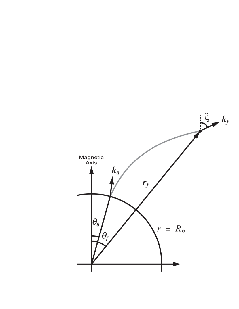
Figure 2: As shown by the halftone line, the slow-mode wave leaves the stellar surface at $(R_{\ast},\theta_{0})$ and follows a magnetic field line. At $(r_{f},\theta_{f})$, it transitions to the fast mode and travels along $\bf k_{f}$.

where $r$ and $\theta$ are the spherical coordinates of the wave packet in the corotating frame, with the dipole axis pointing along the $z$-axis, as illustrated in Figure 2. Here, the 0 subscript denotes values at the stellar surface. The first equation simply says that the wave packet follows the magnetic field lines. The second equation describes how the direction of the wave vector relative to the field line evolves as the wave packet moves down the field line. As the wave moves farther away from the neutron star, the orientation of the wave vector depends less on its initial orientation and increasingly on its displacement from the star.

The strong magnetic field constrains the electrons and positrons to move along the field lines; hence, their density is proportional to the magnetic field strength which, for a dipolar magnetic field, varies as $r^{-3}$. In the corotating frame then, the plasma frequency is given by

$$\omega_{p}^{2}(r)=2\frac{4\pi N_{0}e^{2}}{m}\,\left(\frac{r_{0}}{r}\right)^{3}$$ (5)

where $N_{0}$ is the plasma density at $r=r_{0}$, $e$ is the elementary charge, and $m$ is the mass of the electron. The factor of two reflects the fact that the plasma consists of positrons and electrons. Transforming to the comoving frame introduces a factor of $1/\gamma_{p}$ because of length contraction, giving

$$\omega^{\prime 2}_{p}(r)=\frac{8\pi N_{0}e^{2}}{\gamma_{p}m}\,\left(\frac{r_{0}}{r}\right)^{3}={\omega^{\prime}_{p_{0}}}^{2}\left(\frac{r_{0}}{r}\right)^{3}$$ (6)

where $\omega^{\prime}_{p_{0}}=\omega^{\prime}_{p}(r_{0})$. In reality, the magnetosphere may contain regions where $\omega_{p}$ does not scale in this manner, and refraction may occur into these regions. Our model neglects this possibility.

Knowledge of both $k_{\perp}^{\prime}$ and $\omega^{\prime}_{p}$ at each point on the trajectory allows us to determine which dispersion relation curve the wave satisfies but not the specific values of $\omega^{\prime}$ and $k_{\shortparallel}^{\prime}$. To find these quantities, we note that the wave also satisfies the Lorentz transformation

$$\omega=\gamma_{p}(\omega^{\prime}+\beta_{p}k_{\shortparallel}^{\prime})$$ (7)

where $\omega$ is constant in the geometric-optics limit. Plotted on the same axes as the dispersion relation, this relation corresponds to a line with slope $-\beta_{p}$ and intercept $\omega/\gamma_{p}\omega^{\prime}_{p}$. The intersection of this line with the dispersion relation curve gives us the values of $\omega^{\prime}$ and $k_{\shortparallel}^{\prime}$ for the slow-mode wave at a given radius. Figure 3 shows four pairs of curves, corresponding to distances of ten, twenty, thiry, and forty stellar radii, for a ray following a field line. The dashed curve shows how $\omega^{\prime}$ and $k_{\shortparallel}^{\prime}$ evolve as the ray travels away from the stellar surface.

To find the transition point, we expand equation (3) in powers of $k_{\perp}^{\prime}/\omega^{\prime}_{p}$ with $k_{\shortparallel}^{\prime}/\omega^{\prime}_{p}=1$ to find

$$\frac{\omega^{\prime}}{\omega^{\prime}_{p}}\approx-1+\frac{1}{2}\frac{k_{\perp}^{\prime}}{\omega^{\prime}_{p}}=-1+\frac{3}{16}\frac{\omega}{\omega^{\prime}_{p_{0}}}\theta_{0}\left(\frac{r}{r_{0}}\right)^{2}$$ (8)

Similarly, from equation (7), we have

$$\frac{\omega^{\prime}}{\omega^{\prime}_{p}}=-\beta+\frac{\omega}{\gamma_{p}\omega^{\prime}_{p}}=-\beta+\frac{\omega}{\gamma_{p}{\omega^{\prime}_{p_{0}}}}\left(\frac{r}{r_{0}}\right)^{3/2}$$ (9)

Setting these two expressions equal to each other gives

$$1-\beta+\frac{\omega}{\gamma_{p}{\omega^{\prime}_{p_{0}}}}\left(\frac{r}{r_{0}}\right)^{3/2}-\frac{3}{16}\frac{\omega}{\omega^{\prime}_{p_{0}}}\theta_{0}\left(\frac{r}{r_{0}}\right)^{2}=0$$ (10)

which may be solved numerically for $r/{r_{0}}$.

After the mode conversion, a ray escapes the magnetosphere as a vacuum electromagnetic wave. The angle between the wave vector and the field line is approximately $n_{\perp}\approx(3/8)\theta$, and the angle between the field line and the dipole axis is $(3/2)\theta$. Therefore, after the transition occurs, the wave travels along a line that makes an angle $\xi=(9/8)\theta_{f}$ with the axis of the dipolar field, where $\theta_{f}$ is the value of $\theta$ at the mode transition.

We simplistically assume in our model that the direction of the wave vector and the polarization remain unchanged by the mode conversion. If the two modes couple due to turbulence within the plasma, one would not expect such a conversion mechanism to preserve ${\bf k}$ and the polarization. Clearly, even in this simple model, the direction of the wave vector must change during the transition; because the phase velocities of the two modes are different, the constraints on $\omega$ and $k_{\perp}$ require that the two modes must have different $k_{\shortparallel}$s. The exact manner in which the slow mode maps to the fast mode depends on details of the conversion process, a discussion of which is beyond the scope of this paper.

3 Ray Trajectories

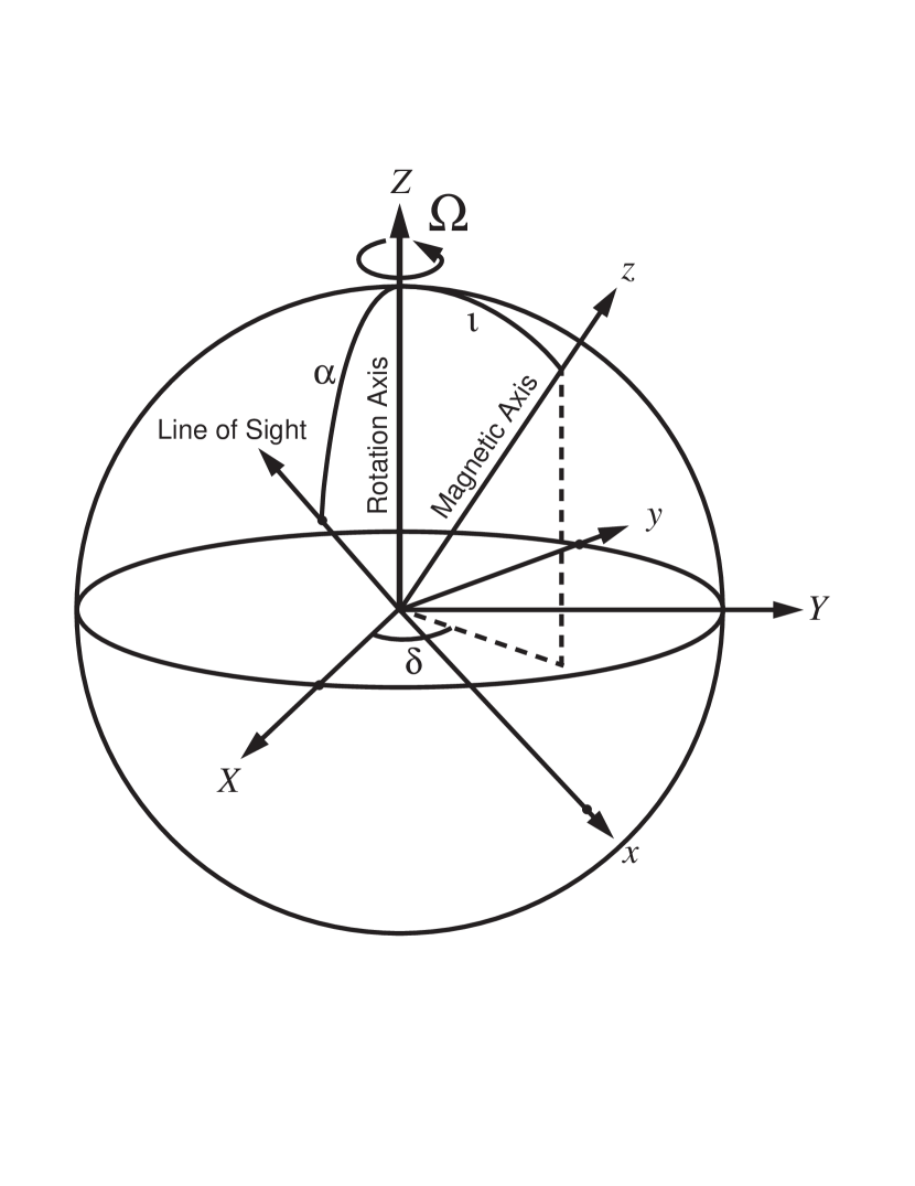
Figure 4: The axis of rotation points along the $Z$-axis. The line of sight lies in the $X,Z$-plane and makes an angle $\alpha$ with the rotation axis, and the direction of the magnetic axis is given by the polar angle $\iota$ and the azimuthal angle $\delta=\Omega t$.

To analyze the path of a wave in the magnetosphere, it is convenient to focus on two reference frames: the observer’s frame and the corotating frame. Figure 4 illustrates the relationship between cartesian coordinates in the two frames. The set denoted by capital letters corresponds to the observer’s frame. The $Z$-axis points along the rotation axis of the pulsar, and the line of sight lies in the $XZ$-plane. The second set, denoted by lower-case variables, lives in the corotating frame. It is related to the first set by a rotation by $\iota$ about the $Y$-axis followed by a rotation by $\delta$ about the $Z$-axis, where the angles $\delta$ and $\iota$ describe the orientation of the pulsar. In this system, the magnetic axis coincides with $z$-axis, and the rotation axis lies in the $xz$-plane. Finally, because we are working with a dipolar field, the corresponding set of spherical coordinates $(r,\theta,\phi)$ in the corotating frame is useful.

The transition from slow to fast mode may occur at a distance which is a significant fraction of the light cylinder radius; consequently, we must take into account the effects of the boost from the comoving frame to the observer’s frame on the wave vector of the ray. The boost changes both the frequency and the direction of the ray. The frequency shift is small, about 1%, and is relatively unimportant. The change in direction, on the other hand, is more significant since the final direction of the ray in the observer’s frame determines if and when the ray will reach the observer.

Each point on the transition surface appears to emit a beam of light with a fixed direction in the corotating frame. In the observer’s frame, the beams rotate with the star. If a beam makes an angle $\alpha$ with the rotation axis, it will sweep across the line of sight when the star has rotated to an appropriate orientation, and the beam will reach the observer.

Figure 5 illustrates the paths taken by several of these rays as seen from the corotating frame. Up to the transition point, the rays follow the magnetic field lines; after the transition, they travel in the directions given by their wave vectors. In the observer’s frame, the rays will travel in straight lines after the transition. In the corotating frame, they will follow spiral trajectories.

4 Constructing the Pulse Profile

To construct the pulse profile, we start with a uniform distribution of rays on the stellar surface centered on the magnetic pole, trace their paths, and select only the ones which will reach the observer. The pulse period is divided into some number of equally-sized bins, and the time of arrival of a ray determines into which bin it goes. Averaging the position angles of the rays contributing to a bin yields the final position angle for that bin.

Each ray carries a Gaussian weighting, with the distribution centered on $\theta_{0}=0$. The width $\sigma_{\theta}$ of the Gaussian corresponds physically to the size of the beam rising from the stellar surface. Appealing to the central limit theorem, we used a Gaussian distribution so that the resulting profile is not that of a single pulse but that of many averaged together. In other words, the model produces the integrated pulse profile.

For a particular orientation of the neutron star, namely $\delta=0$, we calculate for each ray its wave vector $\bf K$ in the frame of the observer. The time of arrival for a ray that will reach the observer is then given by

$$t_{arr}=-\frac{\phi_{K}}{\Omega}-\frac{{\bf R}\cdot\hat{\bf K}}{c}$$ (11)

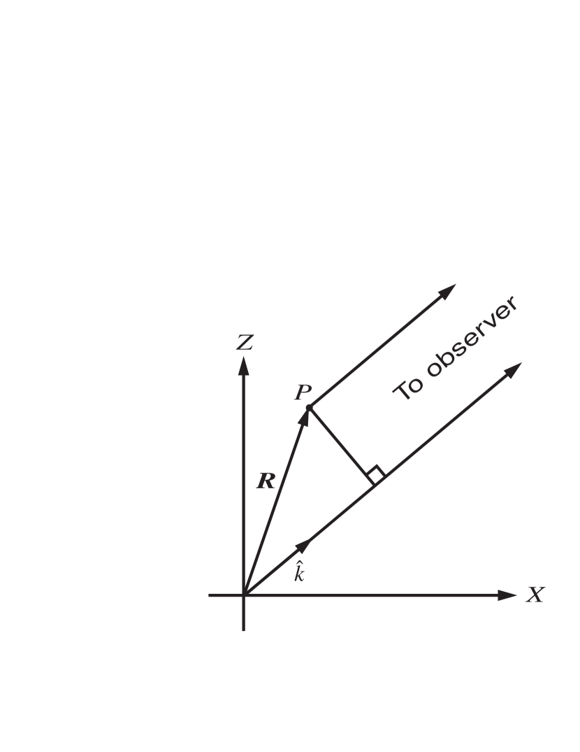
Figure 6: The ray leaving from point P travels a distance ${\bf R}\cdot\hat{\bf k}$ less than a ray from the origin. Hence, it will arrive at the observer a time $\delta t={\bf R}\cdot\hat{\bf k}/c$ earlier.

where $\phi_{K}$ is the azimuthal angle of the wave vector, $\Omega$ is the rotational speed of the pulsar, $\bf R$ is the point where the ray breaks free of the magnetic field line, and $\hat{\bf K}$ is the unit vector in the direction of the wave vector. The first term accounts for the fact that the star must rotate to the proper orientation for the ray to align with the line of sight. The second term arises from the displacement of the transition point from the star, as illustrated in Figure 6. The travel time for the light ray from a pulsar at a distance $D$ is approximately $t=D/c$; the actual travel time differs from this value because the wave decouples from the plasma at a displacement $\bf R$ from the center of the star.

As mentioned earlier, the rotating-vector model plausibly accounts for the characteristic sweep in position angle under the assumption that the polarization reflects the geometry of the dipolar field. The refraction model of wave propagation naturally explains the alignment of the electric field with the field lines because, for both the O-mode and X-mode, the direction of the electric field is determined by the directions of the magnetic field and the wave vector $\bf k$.

For a dipolar field, the rotating-vector model predicts that the position angle $\psi$ will vary according to

$$\tan\,\psi(\delta)=\frac{\sin\alpha\sin\delta}{\sin\iota\cos\alpha-\cos\iota\sin\alpha\cos\delta}$$ (12)

where $\delta=\Omega t$. This relation, however, neglects relativistic and time-of-arrival effects. The transformation from the corotating frame to the observer’s frame changes the direction of $\bf E$. Moreover, because of the second contribution to the time-of-arrival delay, a ray corresponding to an orientation $\delta_{1}$ can arrive before, at the same time as, or after a ray corresponding to $\delta_{2}>\delta_{1}$. These effects may help explain the deviations observed by Krishnamohan & Downs (1983) from the predictions of the basic rotating-vector model.

We obtain the polarization of a ray in the observer frame by calculating the electromagnetic field tensor $F_{\mu\nu}$ for the wave in the corotating frame and then transforming it to the observer frame. To find the electric and magnetic field components in the corotating frame, we define a set of cartesian coordinate axes so that the $z$-axis points along the wave vector and the $x$-axis lies in the $({\bf k},{\bf B})$-plane. The electric field then points along rotated $x$-axis, and the magnetic field, along the $y$-axis.

We have assumed that the electric field of a ray lies in the plane of the dipole field line. Cheng & Ruderman (1979) found that a narrow cone of rays emitted about a field line with initially no average polarization will eventually become nearly completely polarized and that the electric fields will lie in the plane of the dipole field line, if the cone and the direction of the magnetic field become sufficiently misaligned. For radiation due to longitudinal acceleration parallel to $\bf B$, the opening half angle of the cone is of order $\gamma_{p}^{-1}\approx 0.01~{}\rm{rad}$. The angle between the cone and the field line at the transition point is of order $\theta_{f}\approx 0.1~{}\rm{rad}$; hence, our assumption seems reasonable.

5 Results From Applying The Model To The Vela Pulsar

Our model has eight parameters. Six of these describe the pulsar: $R_{\ast}$ is its radial size; $T_{\ast}$, its rotation period; $L_{\ast}$, its spin-down luminosity; $\iota$, the angle between the magnetic field axis and the rotation axis; $\gamma_{p}$, the bulk relativistic factor of the electron-positron wind; and $\sigma_{\theta}$, the width of the beam. The two remaining parameters $\alpha$, the angle between the rotation axis and the line of sight, and $\omega$, the observing frequency, describe the observer.

All of the parameters are set by observations, theory, or the observer except for $\alpha$, $\iota$, $\sigma_{\theta}$, and $\gamma_{p}$. However, observations of polarization often determine the quantity $\alpha-\iota$, and sometimes determine $\iota$ as well. Thus, our model contains, in effect, two or three parameters that can be set to change the pulse shape.

The degree to which refractive effects dominate the propagation of the electromagnetic waves depends mainly upon the plasma density on the open field lines. We calculated this density by assuming that the spin-down luminosity of the pulsar is carried away by the electrons and positrons on the open field lines; thus, the ratio $L_{\ast}/\gamma_{p}$ sets the density of the electron-positron wind at a given radius. We chose to apply the model to the case of the Vela pulsar because its relatively high spin-down luminosity $L_{\ast}=6.918\times 10^{36}~{}\rm{erg~{}s}^{-1}$ and correspondingly dense plasma should emphasize the refractive effects.

Vela’s short $89.30~{}\rm{ms}$ rotation period translates to a light cylinder radius of $4236~{}\rm{km}$. We found that the transitions from slow-mode to fast-mode waves occur within 10% of this distance. Relativistic effects, small as they are, could still have a significant effect on the pulse shape.

We set $\iota$ to $90\arcdeg$ and $R_{\ast}$ to $10~{}\rm{km}$ and chose the values for the remaining parameters $\gamma_{p}=100$, $\sigma_{\theta}=0.020~{}\rm{rad}$, and $\alpha=94.8\arcdeg$ so that the model would produce a reasonable pulse shape for an observing frequency of 2.3 GHz. We did not perform an extensive search of the parameter space to study the effects on the pulse profile.

Figure 5 depicts the paths of several rays to the observer as seen in the corotating frame. In this frame, observers follow paths which encircles the magnetic pole and see a pulse when they cuts across the “spray” of light. From this figure, we also see that observers would measure the size of the pulsar, i.e. the size of the transition surface, to be around 100 km at 2.3 GHz, a result which agrees reasonably well with recent size measurements of Vela. Macquart et al. (1999) obtained an upper limit of 50 km from 660 MHz scintillation data and suggested that the size of the emission region increases with frequency; Gwinn et al. (2000) measured the size of Vela’s emission region to be 440 km; and Krishnamohan & Downs (1983) found a spread in altitude of about 400 km.

Figure 7 shows the intensity profiles obtained from the model for two frequencies and the associated transition surfaces. The dotted curves correspond to 1.4 GHz, and the solid curve, to 2.3 GHz. The larger transition surface at 1.4 GHz results in a wider pulse. A plot of the position angle shows a smooth sweep, somewhat obscured by the break in the curve caused by the coarse graining of the bins. At the start of the pulse, the shape of the curve deviates from the S-shaped curve predicted by the simple rotating-vector model because rays from many longitudes contribute to the leading edge of the pulse.

Figure 8 shows the observed integrated pulse profile for the Vela pulsar at 1.4 GHz. The average position angle sweeps through roughly the same range for both profiles. More interesting, the predicted and observed profiles both appear to consist of the overlap of a strong subpulse followed by a weaker subpulse, although the model did not reproduce the relative strengths accurately. In our model, the presence of two subpulses arises from a combination of three effects.

Every ray reaching the observer emanates from a point on the stellar surface; therefore, we can map a pulse to a curve or a region, if rays from multiple points reach the observer at the same time, on the stellar surface. Moving along this curve corresponds to advancing in time on the profile. Typically, this path starts at some point $(\theta_{0},\phi_{0})=(\Theta_{0},\Phi_{0})$ and while $\phi_{0}$ monotonically decreases, $\theta_{0}$ first decreases, reaches a minimum, and then increases.

Because of the cylindrical symmetry around the magnetic pole, each circle of latitude on the stellar surface has an associated circle of transition points in the magnetosphere. The density of rays reaching the observer is higher when the line of sight grazes one of these circles than when it cuts across the circle at some angle. Hence, the density of rays reaches a peak when $\theta_{0}$ hits its minimum and the path on the stellar surface is tangent to a circle of latitude.

Each ray represents an area element $d\Omega_{0}\approx\theta_{0}d\theta_{0}d\phi_{0}$, so its weight contains a factor of $\theta_{0}$ as $d\theta_{0}$ and $d\phi_{0}$ are fixed in our model. The weight assigned to a ray also has the Gaussian factor mentioned earlier, representing the strength of an average beam. The beam is strongest at the magnetic pole and weakens away from the pole with a characteristic distance specified by $\sigma_{\theta}$.

This combination of weighting factors can easily lead to the appearance of two subpulses. At first, when $\theta_{0}$ is large, the Gaussian factor suppresses the weighting. As $\theta_{0}$ decreases, the weighting at first steadily increases. At some point, the area factor $\theta_{0}$ will begin to dominate, and the weight will decrease, resulting in the first subpulse. After $\theta_{0}$ reaches its minimum, the reverse sequence occurs, generating the second subpulse.

Neither the higher density of rays at smaller values of $\theta_{0}$ nor the weighting assigned to the rays can result in the observed pulse with its asymmetry between the two subpulses. Neither effect nor their combination breaks the cylindrical symmetry. If the density effect enhances one weighting maximum, it will enhance the other one equally. With only these two effects, the observer would always see symmetrical pulse.

The final effect is the time-of-arrival effect, which does break the symmetry. In the corotating frame, the cylindrical symmetry about the magnetic pole results in a transition surface with a reflection symmetry through the x-z plane. The Lorentz boost to the observer’s frame, however, breaks the symmetry by rotating all of the wave vectors in the direction of the boost and, because this rotation affects the time-of-arrival, skews the pulse to the left in the profile. The other contribution to the time-of-arrival delay further skews the pulse to the left; rays from further out on the transition surface take less time to travel to the observer and arrive earlier in the pulse. Also because their transition points are moving faster, they undergo a larger boost, resulting in a larger rotation and causing them to arrive even earlier in the pulse.

Figure 9 illustrates how these effects combine to give the observed pulse. The top plot shows that rays starting near the magnetic pole arrive early in the pulse. The bottom plot shows the weighting with two maxima, but these small variations can not alone account for the large difference in strength between the two subpulses. The superimposed histogram shows that many rays amass near the beginning of the profile. The first subpulse results then from a combination of the first maximum in the weighting and the large number of rays reaching the observer at the same time. The second subpulse arises as the rays arrive at a constant rate but with decreasing weights.

6 Summary

A simple ray-tracing model that assumes a neutron star with a corotating dipolar magnetic field yields results which appear qualitatively consistent with observations. The resulting pulse profile exhibits the general characteristics of the observed profiles; the size of the emission region agrees with recent measurements; and the model naturally incorporates the rotating-vector model if one assumes the mode conversion process does not obliterate polarization information.

The basic nature of the model, moreover, leaves room for refinement. We have neglected the physics in the transition from the slow mode to the fast mode, and an improved model may involve a more realistic momentum distribution for the plasma. Finally, adjusting the weight assigned to each ray by incorporating a more detailed model of the radiation distribution at the surface may yield information about the shape of individual pulses and their variations.

Appendix A Coordinate Transformations From the Corotating Frame to the Observer’s Frame

After solving equation (10) for $r/{r_{0}}$, we can find $\theta_{f}$ using equation (4a). Due to the cylindrical symmetry of the dipole field, transitions occur for all values of $\phi$. For a given value of $\phi$, the transition occurs at the point

$${\bf r}=r(\sin{\theta_{f}}\cos{\phi},\sin{\theta_{f}}\sin{\phi},\cos{\theta_{f}}),$$ (A1)

and the ray has a wave vector

$${\bf k}=\omega(\sin{\xi}\cos{\phi},\sin{\xi}\sin{\phi},\cos{\xi})$$ (A2)

where $\xi=(9/8)\theta_{f}$. The electric field $\bf e$ and magnetic field $\bf b$ are given by

$${\bf e} = (\cos{\xi}\cos{\phi},\cos{\xi}\sin{\phi},-\sin{\xi})$$ (A3a)

$${\bf b} = (-\sin{\phi},\cos{\phi},0).$$ (A3b)

We are working in units where $c=1$. The vectors are normalized as we are not concerned with their magnitudes but only with their directions so that we can determine the polarization of the ray as seen by the observer.

The coordinates in the corotating frame and the observer’s frame are related via two rotations so that

$${\bf R} = (X,Y,Z)=R_{Z}(\delta)R_{Y}(\iota){\bf r}$$ (A4a)

$${\bf\tilde{K}} = (\tilde{K}_{X},\tilde{K}_{Y},\tilde{K}_{Z})=R_{Z}(\delta)R_{Y}(\iota){\bf k}$$ (A4b)

$${\bf\tilde{E}} = (\tilde{E}_{X},\tilde{E}_{Y},\tilde{E}_{Z})=R_{Z}(\delta)R_{Y}(\iota){\bf e}$$ (A4c)

$${\bf\tilde{B}} = (\tilde{B}_{X},\tilde{B}_{Y},\tilde{B}_{Z})=R_{Z}(\delta)R_{Y}(\iota){\bf b}$$ (A4d)

where $R_{Z}$ and $R_{Y}$ are the rotation matrices for rotations by the specified angles about the $Z$-axis and $Y$-axis respectively.

Appendix B Lorentz Transformations

The vector $\bf\tilde{K}$ does not give the wave vector of the ray as seen by the observer; rather, it is the representation of the wave vector as measured in the corotating frame expressed in the coordinates of the observer’s frame. To find the wave vector as seen by the observer, we must apply a Lorentz transformation because the transition point moves with a velocity $\mbox{\boldmath$\beta$}=(\Omega{\bf\hat{Z}})\times{\bf R}/c$.

The components of $\bf\tilde{K}$ parallel and perpendicular to $\beta$ are given by

$${\bf\tilde{K}}_{\shortparallel} = ({\bf\tilde{K}}\cdot\hat{\mbox{\boldmath$\beta$}})\hat{\mbox{\boldmath$\beta$}}$$ (B1a)

$${\bf\tilde{K}}_{\perp} = {\bf\tilde{K}}-{\bf\tilde{K}}_{\shortparallel}$$ (B1b)

where $\hat{\mbox{\boldmath$\beta$}}$ denotes the unit vector in the direction of $\beta$. According to the observer, the ray has a wave vector ${\bf K}={\bf K}_{\shortparallel}+{\bf K}_{\perp}$ where

$${\bf K}_{\shortparallel} = \gamma(\tilde{K}_{\shortparallel}+\beta\omega)\hat{\mbox{\boldmath$\beta$}}$$ (B2a)

$${\bf K}_{\perp} = {\bf\tilde{K}}_{\perp}.$$ (B2b)

and $\gamma=1/\sqrt{1-\beta^{2}}$ is the usual relativistic factor.

We must likewise transform the electric and magnetic fields. The electric and magnetic fields that the observer will see are given by

$${\bf E} = \gamma({\bf\tilde{E}}-\mbox{\boldmath$\beta$}\times{\bf\tilde{B}})-\frac{\gamma^{2}}{\gamma+1}(\mbox{\boldmath$\beta$}\cdot{\bf\tilde{E}})\mbox{\boldmath$\beta$}$$ (B3a)

$${\bf B} = \gamma({\bf\tilde{B}}+\mbox{\boldmath$\beta$}\times{\bf\tilde{E}})-\frac{\gamma^{2}}{\gamma+1}(\mbox{\boldmath$\beta$}\cdot{\bf\tilde{B}})\mbox{\boldmath$\beta$}.$$ (B3b)

The position angle $\psi$ is then given by

$$\psi=\arctan{\left(\frac{E_{Y}}{\sqrt{E^{2}-E_{Y}^{2}}}\right)}$$ (B4)

Figure 1: Plot of the cold plasma O-mode dispersion relation in the rest frame of the plasma for various values of $k_{\perp}^{\prime}/\omega^{\prime}_{p}$, as indicated by the numbers labeling each curve. The upper branch corresponds to the superluminal or fast mode; the lower branch, to the subluminal or slow mode.

Figure 3: A line and a dispersion relation curve are associated with each point in the trajectory of an O-mode wave packet. The intersection of the two yields the waves values of $\omega^{\prime}$ and $k_{\shortparallel}^{\prime}$ at that point. The dashed line shows how $\omega^{\prime}$ and $k_{\shortparallel}^{\prime}$ evolve as the wave propagates away from the pulsar.

Figure 5: These figures show the paths of several rays, as seen in the corotating frame, projected onto the $xz$- and $yz$-planes.

Figure 7: This figure shows model-generated pulse profiles at 1.4 GHz (dotted) and 2.3 GHz (solid) and the corresponding transition surfaces. The pulse period consists of one hundred bins.

Figure 8: The observed integrated pulse profile of the Vela pulsar at 1.4 GHz. We thank S. Sallmen and D. C. Backer for providing these data.

Figure 9: Rays from near the magnetic pole arrive early in the pulse, enhancing the first subpulse.

References

- Arons & Barnard (1986) Arons, J., & Barnard, J. J. 1986, ApJ, 302, 120
- Backer, Rankin, & Campbell (1976) Backer, D. C., Rankin, J. M., & Campbell, D. B. 1976, Nature, 263, 202
- Barnard & Arons (1986) Barnard, J. J., & Arons, J. 1986, ApJ, 302, 138
- Beskin, Gurevich & Istomin (1988) Beskin, V. S., Gurevich, A. V., & Istomin, I. N. 1988, Ap&SS, 146, 205
- Cheng & Ruderman (1979) Cheng, A. F., & Ruderman, M. A. 1979, ApJ, 229, 348
- Cordes (1978) Cordes, J. M. 1978, ApJ, 222, 1006
- Goldreich & Julian (1969) Goldreich, P. & Julian, W. H. 1969, ApJ, 157, 869
- Gallant (1996) Gallant, Y. A. 1996, in IAU Colloq. 160, Pulsars: Problems and Progress, ed. S. Johnston, M. A. Walker, & M. Bailes (San Francisco: Astronomical Society of the Pacific), 431
- Gwinn et al. (2000) Gwinn, C. R., et al. 2000, ApJ, 531, 902, astro-ph/9908254
- Krishnamohan & Downs (1983) Krishnamohan, S., & Downs, G. S. 1983, ApJ, 265, 372
- Lerche (1970) Lerche, I. 1970, ApJ, 162, 153
- Lyne & Graham-Smith (1998) Lyne, A. G., & Graham-Smith, F. 1998, Pulsar Astronomy, (2nd ed.; Cambridge: Cambridge University Press)
- Lyutikov (1998) Lyutikov, M. 1998, Ph.D. Thesis, California Institute of Technology
- Macquart et al. (1999) Macquart, J. P., Johnston, S., Walker, M., & Stinebring, D. 1999, in IAU Colloq. 177, Pulsar Astronomy—2000 and Beyond, ed. M. Kramer, N. Wex, & R. Wielebinski (San Francisco: Astronomical Society of the Pacific), 215, astro-ph/0001368
- Manchester (1975) Manchester, R. N. 1975, Proceedings of the Astronomical Society of Australia, 2, 334
- McKinnon & Stinebring (1998) McKinnon, M. M., & Stinebring, D. R. 1998, ApJ, 502, 883
- Melrose (1996) Melrose, D. B. 1996, in IAU Colloq. 160, Pulsars: Problems and Progress, ed. S. Johnston, M. A. Walker, & M. Bailes (San Francisco: Astronomical Society of the Pacific), 139
- Radhakrishnan & Cooke (1969) Radhakrishnan, V., & Cooke, D. J. 1969, Astrophys. Lett., 3, 225
- Rankin (1983) Rankin, J. M. 1983, ApJ, 274, 333