A radio continuum survey of the southern sky at 1420 MHz

We describe the equipment, observational method and reduction procedure of an absolutely calibrated radio continuum survey of the South Celestial Hemisphere at a frequency of 1420 MHz. These observations cover the area $\rm 0^{h}\leq R.A.\leq 24^{h}$ for declinations less than $-10\degr$. The sensitivity is about 50 mK T_B (full beam brightness) and the angular resolution (HPBW) is $35\aas@@fstack{\prime}4$, which matches the existing northern sky survey at the same frequency.

1 Introduction

The present paper describes the observations of the South Celestial Hemisphere at a frequency of 1420 MHz carried out with one of the 30-m radio telescopes of the Instituto Argentino de Radioastronomía (IAR) at Villa Elisa, Argentina. This continuum survey is intended to complement the northern sky survey (Reich  reich82 (1982); Reich & Reich reich+reich86 (1986)) made with the 25-m Stockert telescope near Bonn to an all-sky radio continuum survey at 1420 MHz.

There are many reasons for carrying out such a survey. Only all-sky surveys allow, under reasonable assumptions, modelling of the emission distribution in the Galaxy. The recognition and study of nearby large-scale features needs survey data as well as investigations of the Galactic emission spectrum when comparing well-calibrated survey data at different frequencies. One important aspect is the determination of the separation of thermal and non-thermal emission in addition to the non-thermal spectral index, which varies with frequency. A spectral index map based on the 408-MHz survey of Haslam et al. (haslam+82 (1982)) and the northern sky 1420-MHz survey by Reich & Reich (1988a ) showed rather unexpected flat spectra towards the anti-centre direction. In a subsequent discussion Reich & Reich (1988b ) proposed an explanation in terms of a cooling–convection halo model. Spectral information for the southern sky is needed to extend and refine this modelling. Galactic foreground emission components and their spectra are also of high interest for cosmic microwave background studies. Meanwhile, a number of sky-horn measurements were available up to short cm-wavelength (e.g. Platania et al. (platania+98 (1998)) and references therein), which give fairly consistent spectral data for the large-scale Galactic emission. However, due to the rather coarse angular resolution of sky-horns, no spatial details can be derived. These require data of higher angular resolution that are provided by single-dish telescopes.

In the following sections we describe the receiver (2), the observation procedure (3), the data acquisition system (4) and the data processing (5). The survey maps will be presented in a forthcoming paper. As examples we show the centre and the anti-centre region in comparison with the northern sky survey to demonstrate its similar performance.

2 Receiving equipment

A deep all-sky radio continuum survey requires receiving equipment having not only sufficient sensitivity to reach the confusion limit of the telescope, but also with the ability to measure the brightest regions of the sky. This is particularly important when regions of both low and high brightness will be crossed by the same scan. The high scanning speed ($10\degr$/min) necessary to perform a large-area survey makes it impracticable to attenuate the signal from brighter objects during the observations. Thus, a receiver should possess a linear dynamic range in excess of 40 dB. In addition, many problems can be avoided if the receiver calibration is constant over long periods of time, even in storage or standby, for observing periods spaced at intervals of several months. The extra requirements of night-time observations avoiding solar and terrestrial interference make telescope scheduling difficult at times.

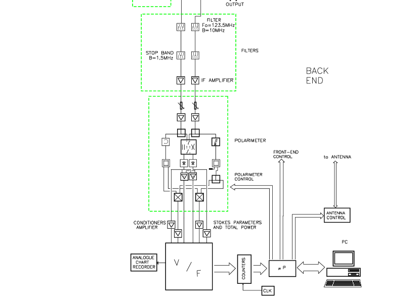
Figure 1: Block diagram of the 1420-MHz continuum receiver at Villa Elisa

A receiver satisfying these requirements was developed and installed in the prime focus of one of the 30-m telescopes of the IAR. Figure 1 shows the block diagram of the receiver system.

The feed is a corrugated horn which, at 1420 MHz, illuminates the dish with a half power beam width of $60\degr$. Its attenuation at the edge of the dish is $-$17 dB. The feed is followed by a ‘turnstile’, a passive device which picks up two linear or circular polarization components, depending on the adjustment. In our case the adjustment was made such as to allow the extraction of the left-hand and right-hand circular polarization of the signal with a polarization isolation larger than 30 dB. The connection between the feed and the turnstile is made by means of a circular waveguide and the two polarization components, extracted from the turnstile, are coupled out by a coaxial probe.

The two circular polarization components are amplified in two separate channels, each of which contains a GaAs FET low-noise amplifier (LNA) with an equivalent noise temperature of 60 K at room temperature. The system noise temperature, including the receiver, ground and sky contributions, is 90 K towards the coldest regions of the sky. Both channels of the receiver were calibrated by measuring the intensity of a standard noise diode, injected through a pair of directional couplers connected between the turnstile and the LNAs, with two optional levels of either 10 K or 50 K. Control signals from the control room can switch the noise source and select its level. The rest of the front-end receiver consists of bipolar amplifiers, interdigital filters, mixers, a local oscillator and an IF-stage with a centre frequency at 123.5 MHz. The IF-signals from the front-end were subsequently filtered with a phase-matched pair of filters and fed into an IF-polarimeter. This device was supplied by the MPIfR, Bonn, where similar polarimeter systems are used at the Effelsberg 100-m telescope (e.g. Schmidt & Zinz schmidt+zinz90 (1990)). The output is proportional to the four Stokes parameters I, V, U and Q. The linear polarization parameters U and Q are obtained from the in-phase and quadrature analogue correlation of the left-hand and right-hand circular signals coming out from the channels A and B of the receiver. The remaining two parameters, I and V, are formed from the sum and difference of the detected input signals. The receiver front-end is thermally controlled to a temperature of $20\degr\pm 2\degr$ C which results in a gain stability of about 0.1 dB for the system during four hours of observations. Special care was taken to match the cable lengths from the noise source to the directional couplers and from the local oscillator to the mixers. Also, in order to minimize the phase drift in the polarimeter due to differential changes in electrical lengths of channels A and B and to changes in temperature, the underground cables used for IF and LO between the front-end and the control room have low attenuation (Heliax type) and high phase stability. In addition, periodic phase calibrations were made to ensure that the phase tracking between channels was less than 5°. In Table 1 the specifications of the receiver are summarized.

Table 1: Receiver specifications

RF-IF gain	80 dB
Line emission rejection	$\geq 23$ dB
Intermediate frequency	123.5 MHz
Dynamic range	40 dB
Polarization components	Circular
Polarization isolation	$\geq 30$ dB
System temperature	$\sim 90$ K
Gain stability in four hours	0.1 dB
Illumination at the edges of the 30-m
reflector	$-$17 dB
Side lobe level related to the main lobe	$\leq 25$ dB
Back side lobe level	$\leq 30$ dB
Temperature stability within the box	$\leq 2\degr$ C/hour
Phase tracking between channels	$\leq 5\degr$

The four-phase switching system is similar to the one used by Haslam et al. (haslam+74 (1974)) to perform a 408-MHz all-sky survey. With this scheme the receiver front-end cycles through four phases of 4 x 60 msec duration. The phases are:

Phase 1: Antenna signal

Phase 2: Antenna signal + Calibration

Phase 3: Antenna signal + Calibration + $180\degr$

Phaseshift between LHC and RHC

Phase 4: Antenna signal + $180\degr$ Phaseshift

This particular data acquisition sequence was chosen for optimal calibration because it permits simultaneous measurement and reduction of the effects of receiver gain variations, second-order terms in the correlator and variations of the correlator and voltage-to-frequency converters. For proper receiver data and antenna position synchronization and recording, two cycles of four phases were accumulated. An analogue output and a digital display were available for monitoring purposes and interference detection.

3 Observations

The observations were made in the total-power mode in two sequences. Between 1987 and 1989, we used a receiver centred at 1435 MHz avoiding H i line emission. The effective bandwidth was 14 MHz. Additional observations were made during a second period in 1993 and 1994. Due to serious problems with interference around 1450 MHz, the system was tuned at a new centre frequency of 1420 MHz. H i line emission was rejected with a band stop filter resulting in an effective bandwidth of 13 MHz. The major part of the observation was done during the first period. In both periods the observations were made exclusively during night time in order to minimize solar and terrestrial interference. Both periods yielded comparable results.

The data were obtained with the nodding scan technique (Haslam et al. haslam+74 (1974)). The telescope moved continously with a speed of $10\degr$/min between a declination of $-10\degr$ and the southern celestial pole. In azimuth it pointed to the local meridian. That way, the survey covers 24 hours of right ascension spaced by one minute of time with a full sampling for all declinations. The northern limit of the observations provides an overlap of $9\degr$ in declination with the northern sky survey, which has a lowest declination of $-19\degr$. This is essential for the matching of both surveys and improves the quality of data in this region.

As mentioned in Sect. 2, the Stokes parameter U and Q (corresponding to linear polarization) have also been recorded, but have not been reduced so far. However, the polarized intensities at 1.4 GHz at medium Galactic latitudes show unexpected structures almost uncorrelated with total intensities (e.g. Uyanıker et al. uyanik+99 (1999)). Modulation by the interstellar medium in front of highly polarized background emission is the most likely explanation. Therefore, the reduction of the polarization data for the southern sky promises interesting results. We summarize some observational parameters in Table 2.

Table 2: Observational parameters of the Villa Elisa southern sky survey

Antenna diameter	30 m
HPBW (effective)	35$\aas@@fstack{\prime}$4
Aperture efficiency	32.8 %
Observing Periods
1987–1989 (epoch 1)
Centre frequency	1435 MHz
Bandwidth	14 MHz
1993–1994 (epoch 2&3)
Centre frequency	1420 MHz
Effective bandwidth	13 MHz
Coverage	$\rm 0^{h}\leq R.A.\leq 24^{h}$
	$-90\degr\leq\delta\leq-10\degr$
Sensitivity	$\sim 50$ mK TB
	(3 $\times$ rms noise)
Gain scale accuracy	5%
Zero level accuracy
(horn measurements)	0.5 K
(relative to 408-MHz survey)	$\leq 0.2$ K
Pointing accuracy	$\sim 2\arcmin$
S/TB (HPBW=35$\aas@@fstack{\prime}$4, full beam)	11.25 Jy/K
S/TA (HPBW=32′)	11.9 Jy/K
	(hot-cold-measurement)

Radio sources, used as flux and pointing calibrators, were observed each night. Maps of the calibration sources were obtained in declination at right ascension intervals of 1 minute. The main calibration sources used were PKS 0518$-$45 (Pictor A) and PKS 0915$-$11 (Hydra A), for which we adopt flux densities of 65.1 Jy and 42.5 Jy, respectively. Other strong radio sources were used as secondary calibrators. Their fluxes were measured relative to a main calibrator during one night. Table 3 lists 22 calibration sources and their adopted peak flux densities.

Table 3: Peak flux densities S of the calibration sources

Source Name (PKS)	S (Jy)
0023$-$26	9.1
0043$-$42	7.5
0114$-$21	4.1
0131$-$36	7.1
0213$-$13	4.4
0320$-$37 (For A)	82.5
0453$-$20	4.7
0518$-$45 (Pic A)	65.1
0741$-$67	3.9
0814$-$35	10.8
0915$-$11 (Hyd A)	42.5
1018$-$42	4.3
1123$-$35	2.3
1302$-$49	7.1
1333$-$33	12.0
1504$-$16	3.1
1610$-$608	60.0
1730$-$13	6.2
1938$-$15	6.5
2058$-$28	5.4
2152$-$69	32.0
2211$-$17	8.6

4 The data acquisition system

The data acquisition system used was built around two small microcomputers: a Commodore 64 (C64) and an IBM PC connected through a serial RS 232 channel transmitting in full duplex mode with a speed of 4800 bauds. This system separates signal and calibration, suppresses a radar signal from the neighbouring international airport of Buenos Aires (Ezeiza), and provides antenna position acquisition and control. In addition the separated data streams (approximately 100 bytes per second) were converted into a tabulated scan array, where a weighted sum of the data was formed for points separated in declination by 0$\aas@@fstack{\circ}$25, the ‘tabular interval’, along the length of a scan. The interpolation was achieved using a tapered ‘sin(X)/X’ interpolation function whose width was matched to the telescope’s beamwidth. During the time interval between subsequent scans, where the telescope’s direction changes, the tabular scan was computed, formatted and stored on the IBM PC’s disc and printed out on request. Both the computer hardware and software developed for this survey were adapted from the observations carried out with the 25-m Stockert telescope for the northern sky. The subsequent analysis was made by using the NOD2 software library (Haslam haslam74 (1974)).

The acquisition module, attached to the on-line processing microcomputers, consists of two parts: a) signal conditioning amplifiers and voltage-to-frequency converters (V/F); b) Villa Elisa Interface (VEI) which connects the C64 with the V/F and the antenna positioning system. It performed the integration of each 60 msec receiver phase for each of the four channels and also provided the electronic timing for the four-phase cycle of the receiver front-end.

The signal conditioning amplifiers provided the necessary amplification for the required output levels of the polarimeter channels entering the V/F converter and an offset displacement to achieve the full dynamic range utilization of the V/F converter. The V/F converter, developed at the IAR, has an analogue-to-digital conversion of 100 kHz/V, high linearity and temperature drift stability. Its output is counted in 15 bit counters.

The VEI is connected with two channels: one is an 8-bit parallel interface from the user port of the C64 that allows reading of the 8-byte counter registers of the V/F converter, and the other one is a serial RS 232 interface built around a Versatile Interface Adapter (VIA) that interfaces with the antenna positioning system to read the actual position and to send control commands. In addition, the VEI provides all the signals necessary to synchronize the real-time acquisition process: integration time of the analogue-to-digital converters, reset of the counters, acquisition of Stokes parameter, antenna position request, noise source injection, phase switching, C64 interrupt and C64 to IBM PC transmission. The reference clock has a period of 60 msec, which is the minimum integration time. This value was chosen to achieve the minimum quantizing error compatible with receiver parameters, the large range of temperatures to scan and the maximum full-scale frequency of the V/F converter. It results in an 1.25$\%$ increase in noise due to digitalization with high 50 Hz frequency rejection. The error of the signal demultiplexing due to the curvature of the gaussian beam is about 0.44$\%$ of the antenna temperature for 60 msec integration time.

5 Data processing

The data processing is divided into three steps,

1. the on-line logging and analysis at the telescope.

2. the off-line analysis to edit and calibrate the data to form a set of raw maps.

3. combination of the maps via the NOD-2 program library (Haslam haslam74 (1974)) and absolute calibration

5.1 The on-line program

A two-level program was installed on the microcomputers. The first level was entered every 60 msec via an interrupt given by the VEI to the C64 and the tasks accomplished during its execution were:

a) Addition of two sets of the four-phase receiver cycles giving an approximate integration time of 0.5 sec.

b) Recording of the current sidereal time and declination from the antenna positioning system and computing of both the signal and calibration demultiplexing for the two total power, the Q and U channels.

c) Transmission of the recorded and computed values to the IBM PC via a 4800 baud RS 232 line.

The second software level provided the weighted tabular scan data. This IBM PC program runs at an asynchronous rate and performed the weighted tabular scan integration at declination intervals of 0$\aas@@fstack{\circ}$25 and adds start, stop times and scan identification number. It displays the scan data in real time. A chart recorder permits an on-line check of both the quality of the astronomical data being processed and the performance of the total system.

At the end of each scan the transmission between both microcomputers was suspended to allow the IBM PC to perform the normalization process, i.e. a noise calibration average over all the scan calibration data and storage of the result on disc.

Figure 2: Flow diagram of the reduction scheme of the 1420-MHz continuum survey

5.2 Off-line analysis and map formation

These reduction steps were performed at the MPIfR, Bonn. A flow diagram of the off-line analysis software is shown in Fig. 2.

An analysis of the raw data, namely TP1, TP2, U and Q and their corresponding calibration channels, revealed a significantly reduced quality of the data in one of the TP channels. Hence an additional coverage in order to reach the required sensitivity was required.

The tabular scan data were sorted in ascending right ascension, calibrated, plotted and inspected and edited for distortions or interference. By scanning in declination along the local meridian the sidelobe structure and the ground radiation will be similar for all scans, and therefore the contribution to the antenna temperature is equal for all points at a given declination. Numerous scans observed in regions of the sky where the emission is nearly constant ($\rm 22^{h}\leq R.A.\leq 3^{h}$) were selected for the two different observing sequences and a lower envelope fitted to these data to determine the characteristic of the ground radiation. In the course of determining the ground radiation curve for the observation period 1993/1994 it became clear that this sequence had to be divided into two intervals. Figure 3 shows the ground radiation profiles for UP and DOWN scans at the three different observation periods.

We have no quantitative explanation as to why the ground radiation profiles are different for the three epochs nor why these curves show a different behaviour for UP- and DOWN-scans in period 2&3. Small systematic changes of the system temperature depending on elevation seem to be the most likely reason. These profiles were subtracted from each observed scan before applying the baseline correction procedure. In order to establish a consistent zero level for the observations, the temperature scale and zero level were found by comparison with the absolutely calibrated Stockert 1420-MHz survey in the overlapping area between $-19\degr$ and $-10\degr$ in declination. Each scan was corrected for the skew (‘nodding’) angle and precessed to equatorial coordinates epoch 1950.0. In the common declination range the mean temperature was calculated and compared with the Stockert survey. In this way, we fixed the upper end of a scan. For the lower end, we averaged the data below declinations of $-80\degr$ excluding compact sources and set it to a constant temperature. With this data set first raw maps were computed. The remaining “scanning effects” due to weather conditions and receiver instabilities were removed using the so-called method of unsharp masking (Sofue & Reich sofue+reich79 (1979)). We used an elliptical Gaussian beam of $1\aas@@fstack{\circ}5\times 0\aas@@fstack{\circ}6$ as a smoothing function. First- and then second-order polynomial fits to the difference temperatures from the smoothed data were utilised to minimize the scanning effects. For the maps observed during the second and third period we used the corrected map from the first observing period as a reference.

Figure 3: Adopted ground radiation profiles for different epochs, which were subtracted from the individual scans. The adopted zerolevels are arbitrary.

We ended up with four maps of the southern sky: two UP-scan and two DOWN-scan. These maps were separately transformed to Epoch 1950. We next computed the difference between the UP-scan map and the DOWN-scan map of each epoch and that between the maps observed in the same scanning direction but of the two different epochs in order to check the pointing accuracy, the temperature scale and whether the subtracted ground radiation profile was correct. We realized that the bandstop filter used during the second coverage to exclude the contribution from the local H i emission was ineffective in eliminating the H i emission from the Small Magellanic Cloud (SMC) and the Large Magellanic Cloud (LMC). Both areas were excluded from the second coverage, i.e. the area covering $\rm 4^{h}40^{m}\leq R.A.\leq 6^{h}$ and $-75\degr\leq\delta\leq-60\degr$ and $\rm 0^{h}20^{m}\leq R.A.\leq 1^{h}20^{m}$ and $-75\degr\leq\delta\leq-70\degr$. The sensitivity was not reduced because the survey is oversampled in this declination range.

The final map was obtained by adding the four maps with the so-called PLAIT-algorithm (Emerson & Gräve emerson+graeve88 (1988)), which in addition destripes the maps. The first coverage was given a double weight.

The full-beam scaling was adopted from the Stockert survey (S/T_B = 11.25 Jy/K), since no large-size antenna pattern could be observed for the IAR 30-m telescope. While the obtained r.m.s.-noise of the present data agrees with that of the Stockert northern sky survey, we note that the southern sky maps show significantly less scanning effects due to the more advanced software and processing power available today.

Figure 4: Area towards the Galactic Centre as observed with the Villa Elisa 30-m telescope. The contours are labelled in K $\rm T_{B}$ (full beam). Contour steps are 100 mK up to 6 K, 250 mK up to 10 K, 500 mK up to 20 K, 1 K up to 50 K and then 2.5 K.

Figure 5: Area towards the Galactic Centre as observed with the Stockert 25-m telescope. The contour steps are the same as in Fig. 4.

6 Absolute calibration

The Villa Elisa southern sky survey is tied to the Stockert northern sky survey in the region of overlap, but any residual large-scale temperature gradient towards the South Celestial Pole requires the determination of absolute temperatures. Absolute temperatures have been measured by Bensadoun et al. (bensadoun+93 (1993)), who have performed sky-horn measurements at various declinations of the northern but also of the southern sky by using the same equipment to determine the cosmic microwave background temperature at 1.47 GHz. The resolution of these data is $30\degr\times 27\degr$, to which we have convolved both the data of the northern and the southern sky. For the northern sky survey, which was absolutely calibrated by a comparison with data of Howell & Shakeshaft (howell+shake66 (1966)) and Pelyushenko & Stankevich (pely+stank69 (1969)) at a declination of $30\degr$, we found a difference to the data of Bensadoun et al. (bensadoun+93 (1993)) of +0.53 K. The derived cosmic microwave background temperature by Bensadoun et al. (bensadoun+93 (1993)) at 1.47 GHz of $2.26\pm 0.19$ K differs by 0.44 K to that assumed by Reich & Reich (1988a ) of 2.7 K. However, there is an additional measurement of the cosmic microwave background of the northern sky at 1.4 GHz by Staggs et al. (staggs+96 (1996)). Their result is $2.65^{+0.33}_{-0.30}$ K, rather close to the adopted temperature of 2.7 K for the northern sky. When subtracting a 2.7 K cosmic microwave background contribution from the 1420 MHz data of the northern sky a reliable spectral index map between 408 MHz and 1420 MHz (Reich & Reich 1988a ) was obtained. Any residual temperature offset at 1420 MHz must be small, e.g. not exceeding about 0.1 K, otherwise a spectral change as a function of intensity results.

We take an offset of +0.49 K (e.g. the mean of both the differences mentioned above) as the best compromise for a correction of the Bensadoun et al. data and added this value to the measurements at declination $-75\degr$ and the equatorial south pole. We end up with the following temperatures, averaged for the specified right ascensions, of 3.30 K ($\rm 4^{h}6^{m}-6^{h}0^{m}$) and 3.28 K ($\rm 3^{h}42^{m}-4^{h}42^{m}$) for $\delta=-75\degr$ and 3.58 K at the south pole ($\rm 7^{h}6^{m}-7^{h}42^{m}$). The temperatures from the Villa Elisa 1420 MHz survey are 3.59 K, 3.58 K and 3.59 K, respectively. Clearly, the temperatures at the south pole agree quite well. However, the temperatures at $-75\degr$ declination are about 0.3 K higher than the sky-horn data and are nearly the same as measured at the south pole. We have at present no explanation for this discrepancy compared to the sky-horn data, although the rather steep ground radiation profiles (Fig. 6) in this declination range might influence the zero-level accuracy locally. There is, however, no indication of a significant temperature gradient towards the South Celestial Pole either from the 45 MHz survey of the southern sky (Alvarez et al. alvarez+97 (1997)) or the 408 MHz all-sky survey (Haslam et al. haslam+82 (1982)), which casts some doubt on the accuracy of the sky-horn data.

7 Example maps

We show two example maps of the Villa Elisa southern sky survey in comparison to the northern sky Stockert data in their regions of overlap. These maps clearly illustrate the comparable quality of the data from both surveys as well as their common zero level and temperature scale.

Figures 4 and 5 display a region of $30\degr\times 20\degr$ along the Galactic plane north of the Galactic centre area. The corresponding T–T plot (temperature versus temperature plot) is shown in Fig. 6. In this region, rather high temperatures were observed and these data are therefore well suited to confirm the temperature scale of the two surveys. As seen from Fig. 6 both scales agree within about 2%.

Figure 6: T–T plot of the data shown in Figs. 4 and 5. The slope of the linear fits is 0.979 or 1.014 for fitting Villa Elisa data versus Stockert data and vice versa.

As a second example we show in Figs. 7 and 8 a section of the Galactic Anti-centre. The emission level is rather low in this area, with just about 1 K above the cosmic microwave background even in the Galactic plane. The two surveys agree within one contour, which is 50 mK T_B.

Figure 7: Area towards the Galactic Anti-centre as observed with the Villa Elisa 30-m telescope. The contours are labelled in K $\rm T_{B}$ (full beam) and the contour steps are 50 mK apart.

Figure 8: Area towards the Galactic Anti-centre as observed with the Stockert 25-m telescope. The contour steps are the same as in Fig. 7.

- (1) Alvarez H., Aparici J., May J., Olmos F., 1997, A&AS 124, 315
- (2) Bensadoun M., Bersanelli M., De Amici G., et al., 1993, ApJ 409, 1
- (3) Emerson D.T., Gräve R., 1988, A&A 190, 353
- (4) Haslam C.G.T., 1974, A&AS 15, 333
- (5) Haslam C.G.T., Wilson W.E., Graham D.A., Hunt G.C., 1974, A&AS 13, 359
- (6) Haslam C.G.T., Salter C.J., Stoffel H., Wilson W.E., 1982, A&AS 47, 1
- (7) Howell T.F, Shakeshaft J.R., 1966, Nature 210, 1318
- (8) Pelyushenko S.A., Stankevich K.S., 1969, Soviet Astron. 13, 2, 223
- (9) Platania P., Bensadoun M., Bersanelli M., et al., 1998, ApJ 505, 473
- (10) Reich W., 1982, A&AS 48, 219
- (11) Reich P., Reich W., 1986, A&AS 63, 205
- (12) Reich P., Reich W., 1988a, A&AS 74, 7
- (13) Reich P., Reich W., 1988b, A&A 196, 211
- (14) Schmidt A., Zinz W., 1990, MPIfR, Technical Report Nr. 67
- (15) Sofue Y., Reich W., 1979, A&AS 38, 251
- (16) Staggs S.T., Jarosik N.C., Wilkinson D.T., Wollack E.J., 1996, ApJ 458, 407
- (17) Uyanıker B., Fürst E., Reich W., Reich P., Wielebinski R., 1999, A&AS 138, 31