Coronagraphic Survey for Companions of Stars within 8 pc

Abstract

We present the technique and results of a survey of stars within 8 pc of the Sun with declinations $\bf\delta>-35\arcdeg$ (J2000.00). The survey, designed to find without color bias faint companions, consists of optical coronagraphic images of the 1′ field of view centered on each star and infrared direct images with a 32^′′ field of view. The images were obtained through the optical Gunn $r$ and $z$ filters and the infrared J and K filters. The survey achieves sensitivities up to four absolute magnitudes fainter than the prototype brown dwarf, Gliese 229B. However, this sensitivity varies with the seeing conditions, the intrinsic brightness of the star observed and the angular distance from the star. As a result we tabulate sensitivity limits for each star in the survey. We used the criterion of common proper motion to distinguish companions and to determine their luminosities. In addition to the brown dwarf Gliese 229B, we have identified 6 new stellar companions of the sample stars. Since the survey began, accurate trigonometric parallax measurements for most of the stars have become available. As a result some of the stars we originally included should no longer be included in the 8 pc sample. In addition, the 8 pc sample is incomplete at the faint end of the main sequence complicating our calculation of the binary fraction of brown dwarfs. We assess the sensitivity of the survey to stellar companions and to brown dwarf companions of various masses and ages.

1 Introduction

In 1992 a brown dwarf companion search began at Palomar with the initiation of a collaboration between T. Nakajima and S. Kulkarni at Caltech and D. Golimowski and S. Durrance at Johns Hopkins. The Hopkins group brought the Adaptive Optics Coronagraph (AOC; Golimowski et al. (1992)) to Palomar to be fitted on the 60” Telescope. The first results of this collaboration are given in Nakajima et al. (1994), which entailed a search for companions of high galactic latitude stars. Companions were distinguished from background stars through statistical arguments based on the distribution of point sources as a function of angular separation from the stars. In 1994, the work expanded to a new sample of nearby stars which were believed to be young. A short description of this sample is contained in Nakajima et al. (1995). This sample was biased toward young stars in an attempt to discover brown dwarf companions, with the assumption that younger brown dwarfs would be easier to detect because they should be brighter (Oppenheimer et al., 2000). The first success of this collaboration was the discovery of a faint companion of the star Gliese 105A (Golimowski et al., 1995). The first success of the young star survey was the discovery of the cool brown dwarf Gliese 229B (Nakajima et al., 1995; Oppenheimer et al., 1995).

Following the discovery of Gliese 229B, we decided that it was of paramount importance to conduct a volume-limited survey for companions. If we continued to pursue the biased sample and found no more brown dwarfs, we would have little to say about the prevalence of companion brown dwarfs without extensive modeling.

For this reason, in late 1994 we began a survey of all the Northern ($\delta>-35\arcdeg$) stars within 8 pc of the Sun to search for brown dwarf companions. Because all of the known stars within 8 pc have measurable proper motions, our survey was designed to find common proper motion companions. We thus observed each star at multiple epochs, if point sources other than the star appeared in the field of view. This permitted us to discern companions simply by measuring the relative offset between the star and the putative companions at each epoch. The common proper motion criterion, almost fifty years old now, is ideal in searches for brown dwarfs because it is intrinsically unbiased by color or other theoretical notions of what a brown dwarf should look like. (Other systematic searches for companions that used the common proper motion criterion are by van Biesbroeck (1961); Luyten (1977); Skrutskie et al. (1989); Simons et al. (1996); Koerner et al. (1999) and Schroeder et al. (2000). See Oppenheimer et al. (2000) for a description of the history of brown dwarf searches.) The common proper motion criterion is the most physically rigorous short-term method for finding companions. (Longer term methods include orbital motion measurements and common parallax measurements, which eliminate the minute possibility that two objects within an arcminute of each other might exhibit common proper motion and yet be physically unassociated.)

This survey is also distinguished from others because it represents the first use of adaptive optics techniques in the study of nearby stars. With our tip-tilt observations dating back to 1992, we greatly predate any other such searches. At the time of this writing, the use of higher order adaptive optics systems is becoming widespread in these sorts of studies (e.g., Delfosse et al. (1999)). The combination of adaptive optics and coronagraphy, and the use of both infrared and optical band passes made our search effective. We demonstrate in §9 and Fig. 19 that the survey covers previously unobserved parts of the companion mass-separation parameter space.

To achieve our goal of a volume-limited survey, we assembled a sample of stars which appear in the Third Catalog of Nearby Stars (Gliese and Jahreiss, 1991) and have parallaxes greater than 0$\farcs$125. The degree of completeness of this sample has been the subject of debate. (See, for example, Reid and Gizis (1997).) We address this issue in depth in §2 where we also present an updated catalog of the stars within 8 pc.

The observations are explained in detail in §3, and a complete description of the sensitivity limits is presented in later sections.

2 The 8 pc Sample

2.1 Culling the Catalog

When we began our survey the best list of stars within 8 pc of the Sun was a subset of the Third Catalog of Nearby Stars (Gliese and Jahreiss (1991); CNS3). The subsequent releases of the Hipparcos Main Catalog (Perryman et al., 1997) and the Yale Catalog of Trigonometric Parallaxes (van Altena et al., 1995) provide important sets of data that modify the census of stars within 8 pc. Ultimately the two new catalogs moved some stars out of, and others into, the 8 pc sample. These catalogs also added a few stars to the sample, which were not in the CNS3. The Hipparcos Catalog did not add any unknown stars to the 8 pc sample because trigonometric parallaxes were only obtained for previously cataloged stars. However, Hipparcos did measure 7 stars in 5 systems whose parallaxes had never before been measured and which place them within 8 pc. The Yale Catalog adds no new stars to the catalog but does provide trigonometric parallaxes for 37 stars within 8 pc which were not measured by Hipparcos. This reduces the number of stars in our sample whose parallaxes are simply inferred from photometry. These so-called photometric parallaxes involve measurements of the colors of a given star. The colors determine the spectral class of the star and, thus, its absolute luminosity. From the absolute luminosity, the distance modulus is calculated. These photometric parallaxes are sometimes inaccurate because of unknown multiplicity and intrinsic scatter in the main sequence which can lead to errors in the distance as large as 30% (Weis, 1984). In the new catalog we assemble here, only 6 stars are included based on photometric parallaxes. These are the only stars within 8 pc in the CNS3 which were not measured astrometrically by the Hipparcos or the Yale surveys.

Pursuant to this discussion we have created a new catalog of stars within 8 pc of the Sun. We believe this comprises the most complete census of the Northern 8 pc volume to date. In our catalog we combine all the stars within the CNS3, Hipparcos and Yale catalogs which have parallaxes greater than 0$\farcs$125. The three catalogs are fully cross-correlated and for each entry in our database we have up to three different parallaxes, although only the most accurate is listed in the catalog presented here. Precedence for inclusion in the final catalog is given to the Hipparcos measurement which is generally more accurate than the Yale measurement (except in the case of star systems Gliese 185AB and Gliese 644ABCD, where the Yale parallax is more accurate). For six of the stars neither Yale nor Hipparcos measurements exist. These stars have photometric parallaxes listed in the CNS3 and we list them to be as inclusive as possible.

To be certain that we have included all the known subordinate stellar and substellar objects associated with these stars, we conducted a search of the literature. Two papers in particular (Delfosse et al., 1999; Reid and Gizis, 1997) provided new companions, some of which have been resolved and some of which were detected through radial velocity studies. Our catalog is not biased in any way as to whether a given companion has been visually resolved. A complete census must be free of these considerations. Therefore, we include all of the companions mentioned in Reid and Gizis (1997) and most of those in Delfosse et al. (1999). We believe that our final catalog is complete as of January 2000 because we have used all of the available resources and studies of the nearby stars.

Our sample includes, therefore, 163 stars, two brown dwarfs (Nakajima et al., 1995; Burgasser et al., 2000) and one indirectly detected planet (Delfosse et al., 1998). These entities are arranged in 111 star systems, 29 of which are double, nine of which are triple, two of which is quadruple and one of which is quintuple.

Table 1 lists all the star systems in the 8 pc sample described above. In this table we give a single entry for every object known within 8 pc. For multiple systems, entries are grouped together and indicate the separation of the subordinate components, along with other vital data. The table is arranged in order of decreasing parallax in milliarcseconds (mas). The “Source Code” field in each entry indicates where the parallax measurement comes from. Companions of stars are indicated by capital Roman letters after the parallax and generally are given in the order in which the components are discovered. An implicit A is given to every principal star in each star system. However, the A is only used if at least component B has been discovered. For convenience we give HD, Durchmusterung, CNS3 or other names for the stars if they are available. This permits easy identification of the stars in astronomical databases.

2.2 Completeness of the 8 pc Catalog

It is important before describing the observations we undertook to estimate how complete our catalog of star systems within 8 pc is.

The simplest way to assess this involves extrapolating the number of stars within 5 pc to the volume of the 8 pc sample. This sort of analysis was conducted by Henry et al. (1997). In their estimation, the CNS3 is complete for stars with $M_{V}<11$ all the way out to 10 pc, although the majority of the incompleteness is in the far-less-studied Southern sky ($\delta<-35^{\circ}$). Their computation involves taking the densities of stars of various absolute magnitudes in the 5 pc volume in the CNS3 (widely used as a benchmark for complete stellar samples) and multiplying by the ratio of the volumes due to increasing the radius of the sample. The 5 pc sample in the CNS3 contains 53 stars with $\delta>-35^{\circ}$. This implies that there should be another $3.096\times 53\pm 7.3=164\pm 23$ stars between 5 and 8 pc. However, there are only 110 such stars known. Since we surveyed 163 stars but expect those to be drawn from a population of 217 $\pm$ 30, we estimate that our catalog is complete to approximately 75% (assuming the stellar densities within 5 pc are correct). Any incompleteness is most likely among the very faintest stars (white dwarfs and late M dwarfs), because they are less likely to have been measured and studied in depth in large scale stellar surveys. In addition, many of the nearby stars were found through large-scale proper motion surveys. Some stars may therefore be missing from the nearby star sample because they have very small proper motions.

Reid and Gizis (1997) argue that the CNS3 is complete to $M_{V}<14$ for $\delta>-30^{\circ}$ within 10 pc. $M_{V}=14$ corresponds to the spectral type M4.5. These considerations permit us to conclude that our sample is complete at least to the spectral type M5, and possibly even fainter. We conservatively claim that the sample is 75% complete and believe that the missing stars are all later than M5 in spectral type.

3 Observations

In pursuit of our goal to image and study brown dwarf companions of stars in our sample, we conducted observations of 107 of the 111 star systems (96% of the sample) in optical and near infrared wavelengths. The observations employed two different imaging instruments, the AOC attached to the Palomar 60” Telescope and the Cassegrain Infrared Camera fitted to the Palomar 200” Hale Telescope.

3.1 Common Proper Motion

We imaged each of the stars at least twice in order to discern faint objects within 30^′′ of each star which display the same proper motion as the stars themselves. Our decision to use the common proper motion criterion was motivated by the plethora of models of brown dwarfs at the time the survey began. These models painted often conflicting depictions of the colors or spectra that brown dwarfs ought to exhibit. (See Burrows and Liebert (1993) for a comprehensive review of the state of these models at about the time that our survey began.) We decided that instead of relying upon one of the models and designing a survey that looked for colors that such a model predicted, we would use a more basic physical argument for finding cool companions.

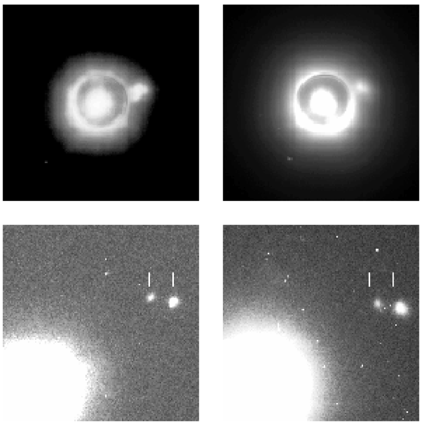
Figure 1: Images of Gliese 105AC (138.72AC). The top two panels are magnified portions of the lower panels. These images were taken in the $z$ band in October 1994 (left) and October 1995 (right). North is up and East is to the left. The star has moved over 2$\farcs$2 between these two epochs and yet the fainter object maintains the same offset from the star in the top panels. This makes it a common proper motion companion. The seeing was better than 0$\farcs$6 in the images, and the astigmatism (which has since been fixed) of the 60” telescope is apparent. The pixel size is 0$\farcs$117. The top images measure 16^′′ on a side. The lower images are 40^′′ on a side. The two white tick marks in the lower left panel serve to mark the positions of the two field stars in 1994. In the lower right panel they are placed in the same location to clearly show that the field stars have moved relative to the central star (which is placed in the same location in the two panels).

The technique we employ here is explained through example in Fig. 1. This figure shows four $z$ band coronagraphic images of the star Gliese 105A (138.72AC). The first two images are magnified portions of the region immediately around the star. These two images were taken a year apart and show a faint second object with the same proper motion. The star moves 2$\farcs$2 yr^-1 permitting extremely easy discrimination between common proper motion companions and background stars. This is demonstrated in the bottom two images, which are larger portions of the same images. In these two, one can clearly see that the two stars to the West do not share the proper motion of the star. We reported this common proper motion companion in the paper by Golimowski et al. (1995).

The error in the measurement of the centroid of a stellar image on a CCD is approximately the angular size of the image divided by the signal-to-noise ratio. (There is a correction factor if the pixel size is much smaller than the image size, but this amounts to a 0.6% correction in this survey. This is because we require every star to be imaged in 1^′′ seeing or better.) In our survey we combine $n$ measurements of each star to improve upon this standard astrometric limit. The effective signal-to-noise ratio of the combined measurement is improved by the factor $n^{1/2}$. At each epoch we have at least two images. With at least two epochs per star, the value of $n$ for most stars is greater than four. The average value of $n$ for all the stars in the survey with other point sources in the field of view is eight. This means that the average centroid error for sources detected at the 5 $\sigma$ level is 0$\farcs$07. All of the stars in our sample exhibit proper motions greater than 0$\farcs$07 yr^-1. Thus we are capable of discerning background objects from common proper motion companions with these observations. In most cases, the proper motions are actually substantially larger than 0$\farcs$07 yr^-1 and the requirement on the astrometric errors is far less stringent than 0$\farcs$07.

3.2 Optical Observations

Optical coronagraphic images of the survey stars were obtained during 25 separate observing runs on the Palomar 60” Telescope between September 1992 and April 1999. These images were obtained with a Tektronix 1024 $\times$ 1024 pixel CCD camera binned in a 2 $\times$ 2 pattern (0$\farcs$117 pixel^-1) attached to the back-end of the AOC. This device consists of a standard Lyot coronagraph (Lyot, 1939) fitted behind a tip-tilt mirror which uses the occulted star as a guide star. The tip-tilt correction provides substantial gains in image resolution on the Palomar 60” Telescope because, there, the majority of the atmospheric disruption of the stellar wavefront resides in tip-tilt energy or, equivalently, image motion. We routinely obtained images with resolutions of 0$\farcs$7 and on six of the observing runs we obtained images at 0$\farcs$45 resolution. The images were taken through the Gunn $r$ and $z$ filters, with additional images taken through the $i$ band if a companion was found. In almost all cases the CCD was exposed for 1000 s. However, for the stars whose magnitude is $V<6$, we were forced to take shorter exposures and to sum these to produce a final image with a 1000 s exposure time. The AOC on the 60” telescope was incapable of guiding on stars fainter than $V\sim 13.5$. For this reason we were unable to observe 13 of the sample stars with the AOC. We had to rely upon the infrared observations of these stars to discern companions. These stars are indicated by the words “too faint” in Table 2.

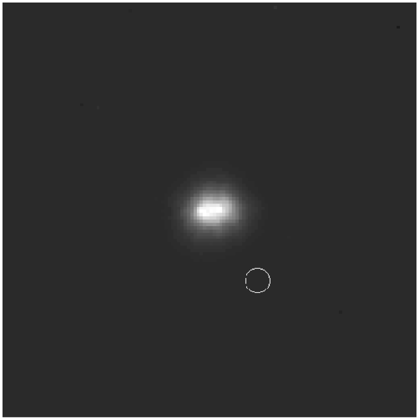
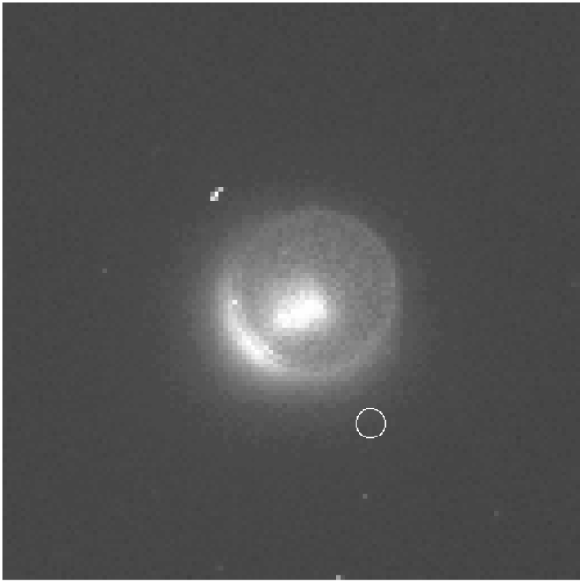
Figure 10: Images of Giclas 089$-$032 (162.00). This star has been resolved into two components. The left image is a 5 s K band image taken in December 1996. The components have a separation of 0$\farcs$75, and North is up with East left. The right panel is a 1000 s $z$ band image taken in January 1998. North is 4.2^∘ left of up and E 90^∘ counterclockwise from there. The two components have been resolved through the semi-transparent coronagraphic mask (4$\farcs$3 in diameter). Here the components have a measured separation of 0$\farcs$71, consistent, within the 0$\farcs$05 error bars, with the infrared offset measured 1.1 years earlier. The star has a known proper motion of 0$\farcs$354 yr^-1. Thus this is a common proper motion pair. The circle in each panel indicates the size of the core of a single star’s point spread function.

The AOC’s focal plane aluminum occulting stop is uniformly translucent in the $r$ and $z$ bands. This permits an accurate measurement of the position of the star in the CCD image. (Without the transparent stop, pinpointing the star would have been impossible because the pupil plane stop eliminates the diffraction spikes of the star.) We used coronagraphic stops 4$\farcs$2 in diameter for most observations, except in the case of the brightest stars where an 8$\farcs$4 diameter stop was used. We claim no sensitivity to faint companions under the stops. However, equal brightness binaries were sometimes resolved under the masks (e.g., Fig. 10).

If a set of $r$ and $z$ band images failed to reveal any sources in the field of view other than the star, we would not reobserve the star. Table 2 lists the dates of all the observations of each star in the sample. In all cases we attempted to acquire images with seeing better than 1$\farcs$0. Seeing worse than this strongly degraded our sensitivity (§4). In all cases we were able to obtain such images at least once for each of the stars observed, and at least twice for those stars with possible companions (i.e., with any other point source in the field of view).

Data reduction involved the subtraction of a bias frame from each of the science images, division by a flat field image obtained using the 60” dome and a flat field lamp, and the removal of cosmic rays (easy to identify in these images because of the very small plate scale). The images were then inspected by eye. In most cases this was sufficient to ascertain whether common proper motion companions were present. However, for the stars whose proper motions are small, additional work was required to distinguish field stars from common proper motion objects. Because the central occulting mask of the coronagraph was somewhat transparent, we were able to centroid the light of the survey star to ascertain its position in the images. Simple centroiding of the other point sources yielded pixel locations as well. These were converted into angular separations in arcseconds by using the observing run’s plate scale and detector orientation. These were determined with the astrometric calibrator fields as explained in §3.4.

3.3 Infrared Observations

Direct infrared images of each of the sample stars were obtained with the D78 Cassegrain Infrared Camera on the Palomar 200” Telescope during 15 observing runs between May 1995 and March 1999. We allowed the stars to saturate the central part of the 256 $\times$ 256 InSb array (0$\farcs$125 pixel^-1). The field of view in these images was approximately 32$\farcs$  Our imaging technique entailed the use of the J and K filters with two types of exposure through each filter. The first type involved a total of five coadds of 1 s exposure time. These images were meant to reveal close binaries with a dynamic range on the order of five to eight magnitudes (depending on the seeing). The second type of exposure used five coadds of 10 s. These exposures were designed to detect fainter companions outside of a 3^′′ radius from the star. In each case a sky frame was taken immediately after the data image was acquired. The sky frame was taken in the same manner as the data image, but with the telescope pointed 50^′′ to the N or E. In some cases we changed this distance because of the presence of a rather bright source in the sky frame.

As with the optical observations, if no objects other than the star appeared, we would not observe the star a second time. In addition the seeing requirement of $\leq$ 1$\farcs$0 for the infrared observations was identical to that for the optical images (see above).

The data reduction for the infrared images involved the subtraction of the sky frame from the “on-source” frame. Subsequent division by a flat field (acquired from the twilight sky during each observing run) permitted the more detailed examination of the images. As with the optical data, visual inspection of the images was usually enough to discern common proper motion companions. In cases where more accurate measurements were necessary, we needed to pinpoint the location of the survey star. This could not be done through centroiding because all of the stars’s images were saturated. Fortunately, we could use the diffraction spikes in the infrared images (absent in the optical images because of the pupil plane apodizing mask in the coronagraph). By fitting the unsaturated parts of the two diffraction spikes with perpendicular lines, we were able to localize the star with an accuracy of better than a third of a pixel. (We confirmed this through short unsaturated exposures of some of the fainter stars in the sample while the telescope guided on a field star. The low frequency tip-tilt system on the f/70 secondary mirror of the 200” telescope guides with an accuracy of better than 0$\farcs$03 over 20 min.) This stellar position on the detector was then used, along with centroids of the light from putative companions, to compute offsets between the objects. These were converted into angular offsets in arcseconds by using the plate scale as described in §3.4.

3.4 Astrometric Calibration

In order to obtain the accurate astrometric measurements of the offsets between the central star and its putative companions, we made observations of calibration fields during each observing run. These fields contained six to ten stars whose relative positions are known within a few milliarcseconds. We used these fields to determine that the astrometric distortion on the face of the CCD chip used in the AOC observations is smaller than 0$\farcs$01 over the whole chip. In the infrared observations the distortion is almost a full pixel near the edges of the array. This distortion is constant with time. Because we centered the stars in the same position on the infrared array at each observing run, the comparison of astrometric measurements is valid, despite this image distortion. We did not use relative astrometry measured on the infrared images in conjunction with other measurements made on the AOC images. For these reasons we applied no astrometric distortion correction in our measurements of relative offsets between stars.

For all of the infrared observing runs, the data were taken with the Cassegrain ring angle precisely set to place North up and East left on the array. This prevented complications in astrometric measurements that would arise from using arbitrary position angles of the array with respect to the cardinal directions.

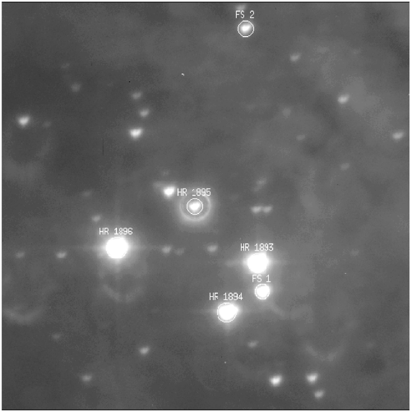
Figure 2: The Trapezium astrometric calibration field. The stars marked with circles and numbers are the stars listed in Table 3 and are the ones used to conduct the calibration. The image measures one arcminute on a side. North is down and East left.

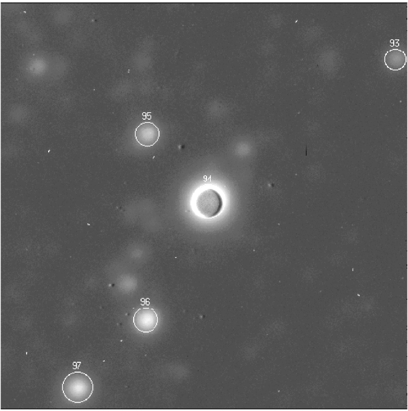
Figure 3: The M5 astrometric calibration field. The stars marked with circles and numbers are the stars listed in Table 4 and are the ones used to conduct the calibration. The images measure one arcminute on a side. North is left and East down.

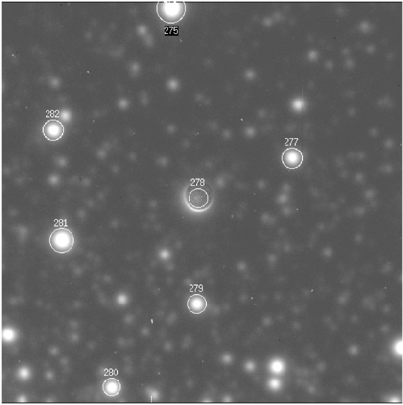
Figure 4: The M15 astrometric calibration field. The stars marked with circles and numbers are the stars listed in Table 5 and are the ones used to conduct the calibration. The image measures one arcminute on a side. North is left and East down.

For every AOC observing run we would observe whichever of the three astrometric calibration fields (listed in Tables 3, 4 and 5) was visible. In each case we would place the star shown in the center of each of Figs. 2, 3 and 4 in the center of the field of view. This star was used for guiding and rapid tip-tilt image motion compensation. From the images—500 s $r$ band exposures—we were able to determine precisely the plate scale and the rotation of the CCD on the plane of the sky. We found that the plate scale was extremely stable in both instruments (despite the fact that the CCD camera used on the AOC was taken apart and reassembled twice between the starting and ending dates of the survey). The accurate positions of the stars in these fields are from Cudworth (1979) for M5, Cudworth (1976) for M15 and McCaughrean and Stauffer (1994) for the Trapezium.

Figs. 2, 3 and 4 show each of the three calibration fields and Tables 3, 4 and 5 give the positions of the stars used for the astrometric calibration.

4 Detection Limits for Each Star

Typically in imaging surveys assessing the sensitivity of the images and the survey as a whole simply involves a determination of the limiting magnitudes of the images. However, in this case the problem is somewhat more complicated.

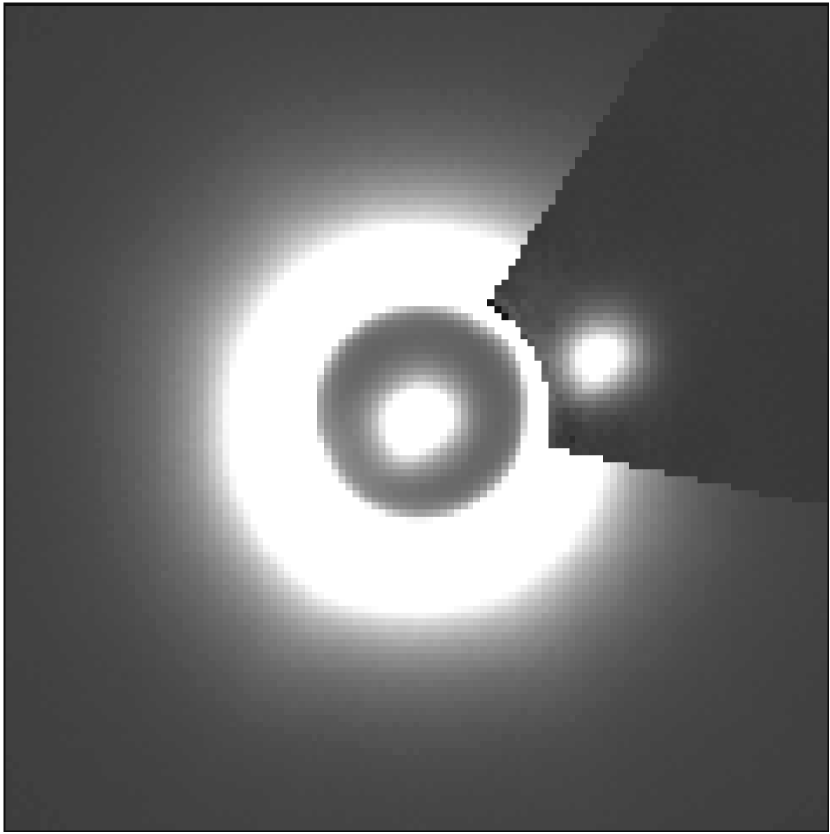
Figure 5: Image of Gliese 105AC. This image, taken through the $i$ band in October 1993, shows only the inner 14$\farcs$5 $\times$ 14$\farcs$5 piece of the larger AOC image. North is up and East to the left. The occulting mask (somewhat transparent) is 4$\farcs$3 in diameter and reveals the core of the star’s seeing disk. Outside the occulted region, part of the seeing disk has been modeled and subtracted to make the companion stand out better. This is unnecessary in order to see the companion, however, as shown in Fig. 1. This image demonstrates the huge dynamic range possible with the AOC. Only 3$\farcs$3 from a star with $i=7.03^{m}$ we detected, with ease, a very low-mass star with $i=12.6^{m}$ with a signal-to-noise ratio of several thousand. We could have detected a companion at this separation in this image as faint as 18.5^m, indicating a dynamic range of 11.5^m at 3$\farcs$3. (From Golimowksi et al. 1995.)

The presence of the bright star in our images means that over much of the field of view the sensitivity is limited by the light of the star and not the sky background (or read noise as was the case for speckle interferometric surveys of these stars; Henry and McCarthy (1990)). However, this survey extends into uncharted parameter space because the coronagraphic technique suppresses a substantial portion of the starlight. The image shown in Fig. 5 illustrates this with the Gliese 105 AC system.

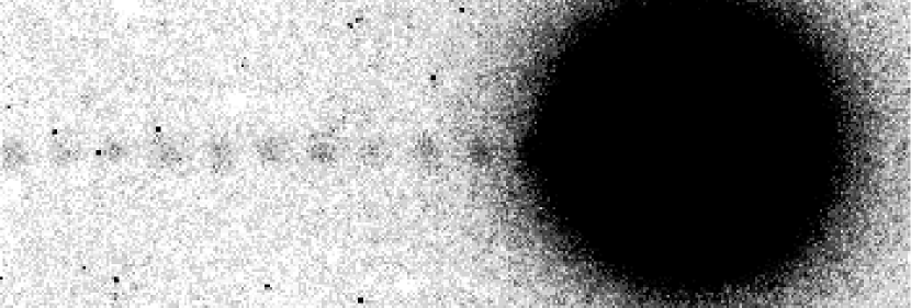
Figure 6: Example of the sensitivity curve determination technique. The images shown are part of a $z$ band coronagraphic image of Giclas 192$-$013 (132.10). The artificial point sources are visible to the left of the star and are placed at regular intervals of 20 pixels. The grayscale stretch shows the lowest light levels, permitting visibility of the large-separation artificial sources while excluding the sources close to the star. The image measures approximately 40^′′ $\times$ 10$\farcs$  The sensitivity curve derived from this image is the lowest one in Fig. 8.

We have measured the detection limits for each star in the survey as a function of angular separation from the central star. To do this we took the images of each star with 1$\farcs$0 seeing or better—the acquisition of such images was a survey requirement (§3)—and inserted artificial point sources at an array of separations from the star. These artificial point sources were generated with appropriate Poisson noise statistics and angular sizes to match the seeing conditions. The magnitudes of these artificial stars (calibrated to the photometric standards used during the relevant observing run) were set so that each artificial star was just visible to the eye. From these magnitudes, the sensitivity curve is derived. An example of this is shown in Fig. 6.

From this procedure, we had a measurement of the faintest source visible at a set of about 10 to 15 radii from the star. Using a spline interpolation between these points, we derived the magnitude limit for $r$, $z$ and J as a function of radius measured from the star. In each band we have individual curves of this nature for each central star in the survey. These curves are summarized in Figs. 7, 8 and 9, where we have displayed representative curves for various star brightnesses in each bandpass.

There are several important effects documented by the curves in Figs. 7, 8 and 9. The most obvious is that the $z$ band imaging is the most sensitive, achieving a maximum dynamic range of 15.5 magnitudes at 10^′′, while, in addition, even the brightest companions can be imaged inside the 5^′′ radius. In comparison, the J band has no sensitivity at the 5^′′ radius for the bright stars and only achieves a maximum dynamic range of 13 magnitudes. What is even more important is the large, slowly-eroding wing of the point spread function in the J band. The $r$ and $z$ bands do not have nearly as much of this broad wing primarily because of the pupil-plane stop in the coronagraph. This stop is designed specifically to depress the wings of the stellar point spread function.

5 Detection Limits for the Survey

From the observational point of view, the curves in Figs. 7, 8 and 9 are the ultimate measure of the sensitivity of our survey. These curves parameterize the sensitivity for every star in the sample. However, it is of paramount importance to convert the information in Figs. 7, 8 and 9 into statements about the survey as a whole and in terms of physical, not observational, parameters. For example, can we safely claim with this data that for all the stars within 8 pc we would have detected any unknown stellar companions in orbits between 3 and 200 AU?

To address this issue, we use the curves found in the previous section to determine the number of surveyed stars for which we could have detected a companion of a given magnitude at a given separation. This information is expressed in terms of the fraction (or percentage) of the total number of stars imaged as a function of magnitude and physical separation in AU. To do this, we systematically went through the catalog of stars. For each star, we took the relevant sensitivity curve, as derived in the previous section, and converted the magnitude scale into absolute magnitudes, using the parallax of the star. We also converted the angular scale into physical separation in AU by dividing by the parallax in arcseconds. Then, we tested whether companions with a set of magnitudes in each band and a set of separations would be visible in our images. By doing this exercise for every star observed, we ended up with a tally of the number of stars, as a function of magnitude and separation, for which the analysis showed that a companion would be visible.

This analysis was done for each of the $r$, $z$ and J bands. (The K band sensitivity curves are essentially identical to the J band curves so we did not independently conduct this analysis for K band.) The results are shown in Tables 6, 7 and 8.

The drop off in the survey sensitivity at large physical companion separations is due to the varying physical field of view caused by the distribution of parallaxes of the stars in the survey. In the J band there is no sensitivity outside of 120 A.U., for example, because the field of view is 15^′′ and the minimum parallax is 125 mas.

In Tables 6 through 8, we have drawn a horizontal line at the approximate absolute magnitude of a 0.08 M_⊙ star. If the hydrogen burning mass limit is 0.08 M_⊙, then all stellar companions must be brighter than the absolute magnitude indicated by the line. Brown dwarfs can be brighter than this line if they are young, but objects below this line must be brown dwarfs and not stars. There are some indications that the hydrogen burning mass limit may not be 0.08 M_⊙. We refer the reader to Gizis et al. (2000) and references therein for observational evidence.

6 Sensitivity to Stellar Companions

We now extend the analysis from the previous section. Instead of discussing the survey sensitivity in terms of observational quantities, we relate those quantities to known properties of stars. This allows us to determine the ability of the survey to find stellar companions of the survey stars. A stellar companion at the minimum mass for hydrogen burning (0.08 M_⊙; Burrows et al. 1997) has absolute magnitudes of $M_{r}=17.4$, $M_{z}=14.9$ and $M_{J}=11.5$. These magnitudes are determined by averaging the photometry of several of the objects known to be at the minimum stellar mass (Henry and McCarthy, 1993). (It is important to note, however, that the exact location of the “hydrogen burning mass limit” is not precisely known. For example, Gizis et al. (2000) suggest that some L-dwarfs might be hydrogen burning and yet have masses below 0.08 M_⊙.) We now use these measurements to make a single table showing the sensitivity to a minimum mass star in each of the bandpasses. The result is shown in Table 9.

What this table demonstrates is that the combination of the infrared and optical imaging permits the detection of any stellar companion at separations greater than 10 AU. We note that for the smaller separations, J band is most sensitive. $z$ band is more sensitive than J band at the higher separations. This is primarily due to the drop in coverage at large separations in the J band (where the field of view is only 32^′′).

Indeed, we have detected six new stellar companions of these stars. These are described below.

7 New Companions

In the course of our observations we have discovered or confirmed seven new companions of nearby stars. Three of these stars, originally included in the 8 pc sample have been removed from the sample because of new and more accurate trigonometric parallaxes. The new companions belong to the following systems: Gliese 105 (138.72), Giclas 089$-$032 (162.00), Gliese 229 (173.19), Giclas 041-014 (224.00), LP 476$-$207, LP 771$-$095 (LTT 1445) and LHS 1885 (Giclas 250$-$031). Only Gliese 229B is substellar. The last three in the list are no longer part of the 8 pc sample, which means that four of our new companions are in the 8 pc sample. Since Gliese 105AC (Fig. 1) and Gliese 229AB have been reported and described in detail elsewhere, we simply refer the reader to Golimowski et al. (1995) for Gliese 105AC and Nakajima et al. (1995), Oppenheimer et al. (1995), Matthews et al. (1996), Golimowski et al. (1998) and Oppenheimer et al. (1998) for Gliese 229AB. Below we describe the other companions.

7.1 Giclas 089$-$032 (162.00)

This star, with no trigonometric parallax measurement, is listed in the CNS3 with a photometric parallax of 162.00 mas and a spectral type of M 5. The Palomar survey has resolved the star into a binary of equal magnitude. It was noted as a double source with 0$\farcs$7 separation in Henry et al. (1997), but they had no information to determine whether the two components were physically associated. In our coronagraphic images taken in January 1998, we resolve the two components under the semi-transparent focal plane mask. The short infrared images also barely resolve the components. With images taken between December 1995 and January 1998 and the known proper motion of the star, 0$\farcs$354 yr^-1, we have ascertained that the two components exhibit the same proper motion and no measurable change in relative offset during this time span. Fig. 10 shows several of our images. Our measured separation is 0$\farcs$73.

7.2 Giclas 041$-$014 (224.00)

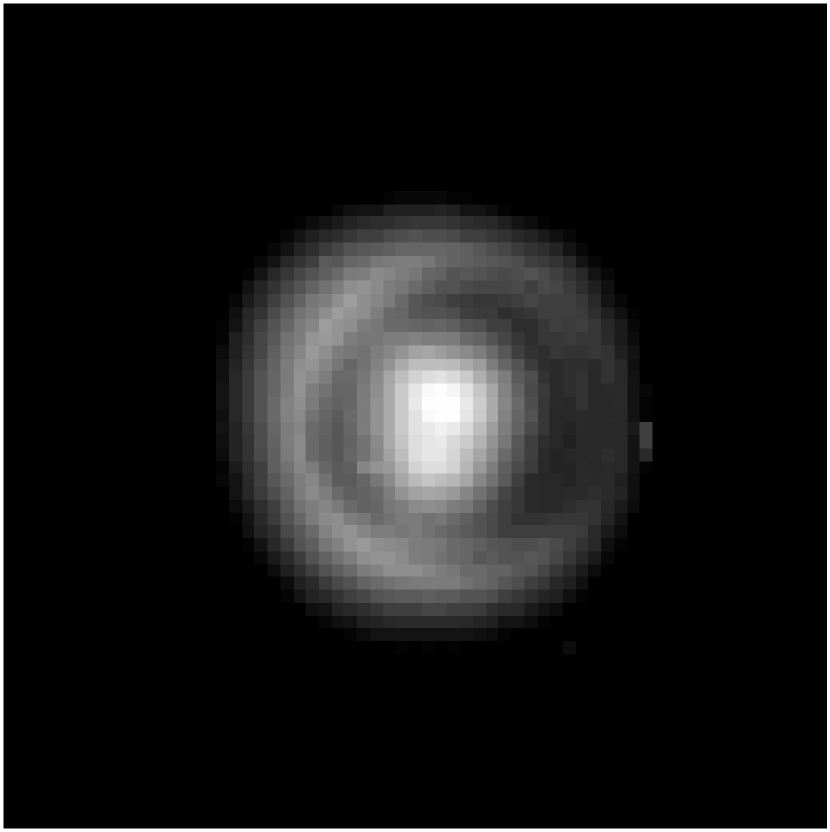
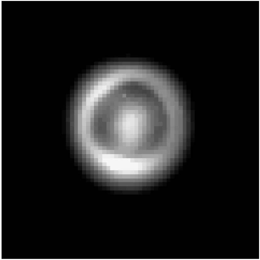
Figure 11: Images of Giclas 041$-$014. This star has been resolved into two components. The left image is a 1000 s $z$ band image taken in November 1996. The components have a separation of 0$\farcs$47 $\pm$ 0.05. North is left and East up. The right panel is a 1000 s $r$ band image taken in March 1998. North is left and East is up. The two components have been only marginally resolved here through the semi-transparent coronagraphic mask (4$\farcs$3 in diameter), the edge of which is visible because of the spillover of light from the stars. Here the components have a measured separation of 0$\farcs$52 $\pm$ 0.1, consistent, within the error bars, with the offset measured 1.25 years earlier. The star has a known proper motion of 0$\farcs$459 yr^-1. Thus this is a common proper motion pair.

Giclas 041$-$014 is a star with a photometric parallax of 224 mas. There is no trigonometric parallax measurement for this star. Reid and Gizis (1997) report that this object has a spectroscopic companion of approximately equal mass. Delfosse et al. (1999) have determined the orbit of this companion (with a period of 7.6 days). However, Delfosse et al. also claim to have resolved a third component of the system with adaptive optics images. They did not publish a confirmation of common proper motion for this object. We have determined that it is a physical companion. They determine a separation of 0$\farcs$62 and a difference of 0.5 magnitudes at K band. This star, which is listed in Table 4.1 as a binary, was included in our survey. We observed it eight times over the duration of this project. Only two of our observations were capable of resolving this putative companion. Both observations were with the AOC in extremely good seeing conditions where the corrected image size was 0$\farcs$45 and 0$\farcs$50. We resolved the companion and measured offsets of 0$\farcs$47 in November 1996 and marginally resolved the companion at 0$\farcs$52 in March 1998. (The standard errors discussed in §3.4 apply to the November 1996 measurement. However, since we only marginally resolved the two components in March 1998, we suggest that the error on that measurement is $\pm$ 0$\farcs$1.) Despite the marginal resolution in March 1998, the expected change in relative offset of this star over this period of time is about 1$\farcs$  Thus, if it were a background object, we would have easily measured this large change in the offset. The magnitude difference in $z$ band is approximately 1.6. Fig. 11 shows the November 1996 $z$ and the March 1998 $r$ band images. In the case of this star (all three components of which are included in Table 1), there was also a faint field star about 9^′′ to the NW. This star’s relative offset between these epochs changed approximately 1^′′, consistent with the 0$\farcs$459 yr^-1 proper motion.

7.3 LP 476$-$207

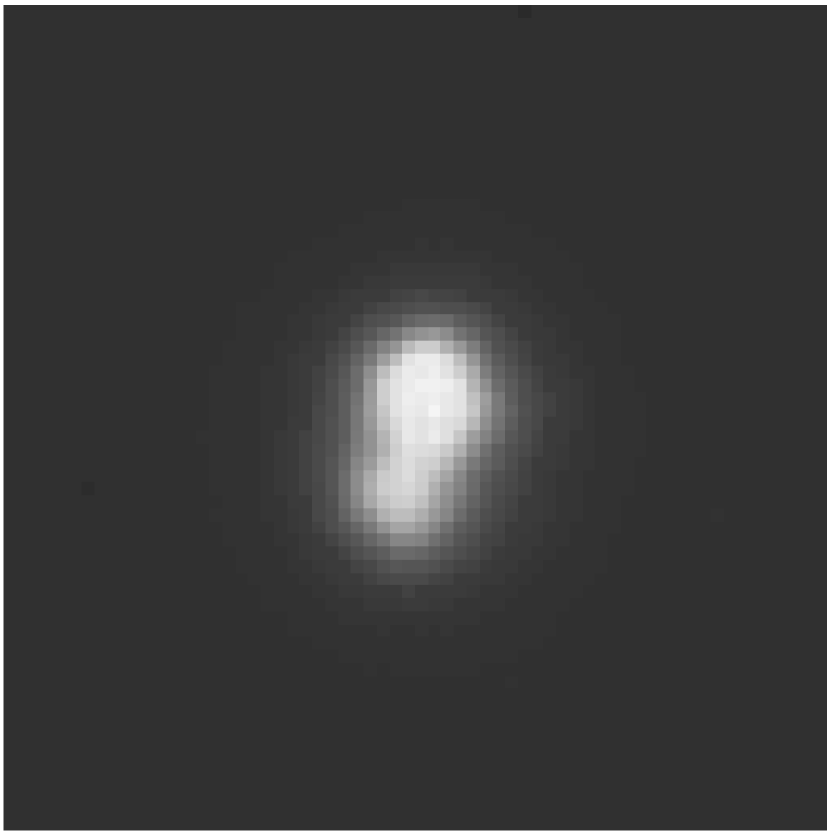
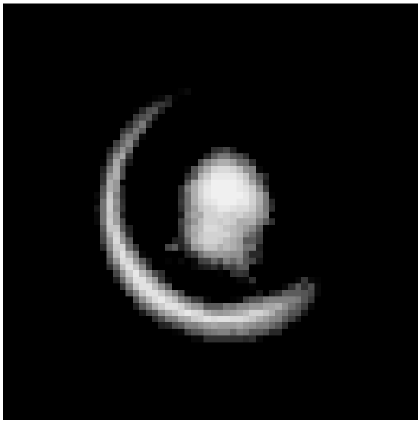
Figure 12: Images of LP 476$-$207. This star has been resolved into two components. The left image is a 5 s K band image taken in October 1996. The components have a separation of 1$\farcs$03. North is up and East is left. The right panel is a 1000 s $z$ band image taken in January 1998. North is up and East is left. The two components have been resolved through the semi-transparent coronagraphic mask (4$\farcs$3 in diameter), the edge of which is visible because of the spillover of light from the companion. Here the components have a measured separation of 0$\farcs$99, consistent, within the 0$\farcs$05 error bars, with the infrared offset measured 2.24 years earlier. The star has a known proper motion of 0$\farcs$0837 yr^-1. Thus this is a common proper motion pair.

This M 4 star was given a photometric parallax of 142 mas in CNS3. The subsequent Hipparcos measurement of 31.20 mas places it well outside the 8 pc sample. Part of the reason that the photometric parallax is so incorrect must be due to the presence of the companion we have found. Even though this star is no longer in the 8 pc sample, it was in our original catalog, so we observed it. We found a common proper motion companion about 1 magnitude fainter in K band than the primary star. This companion is located 1$\farcs$03 from LP 476$-$207. The two images in Fig. 12 show a 5 s K band image from October 1996 and a 1000 s $z$ band image from January 1998. The proper motion of this star is only 0$\farcs$0837 yr^-1, which is less than 1 pixel yr^-1 in these images, but the 2.24 yr baseline permits easy identification of this fainter object as a common proper motion companion. Henry et al. (1997) also identified this star as double, without further information to determine that the two are physically associated. Delfosse et al. (1999) have confirmed the results above, measuring an offset of 0$\farcs$97 and a magnitude difference of 0.9 in the K band. However, because of the single epoch nature of their observation, they were unable to state with certainty that this was a physical companion of the star. Interestingly, they also reported the detection of an unresolved spectroscopic companion of the primary star.

7.4 LP 771$-$095 (LTT 1445)

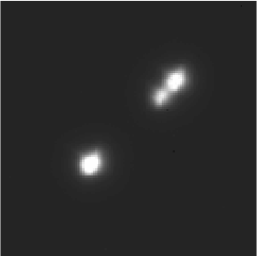
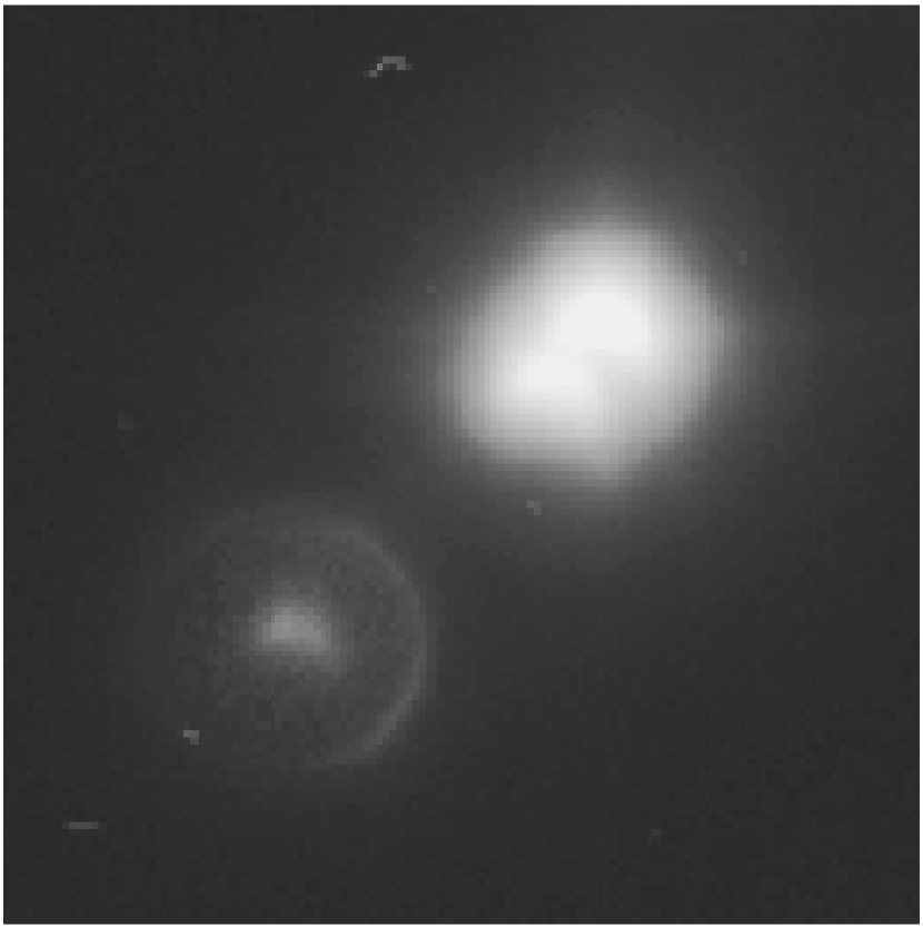
Figure 13: Images of LP 771$-$095 triple system. This star is a known binary (the two outer stars), but we have found a third stellar component of the system which shares the proper motion of the other two (LP 771$-$095 and LP 771$-$096). On the left is a 5 s K band image taken in October 1996. The components have a separation of 1$\farcs$12 and 7$\farcs$23 from the star LP 771$-$095, which is to the upper right in the images. North is up and East is left. The right panel is a 1000 s $z$ band image taken in October 1995. North is up and East to the left. LP 771$-$096 is under the mask in this case. All three components are clearly visible. Unfortunately, the astigmatism of the Palomar 60” telescope is also apparent. In order to measure accurate astrometry on this image, we used only the light in the brightest part of the point spread function. Our astrometry matches that from the infrared images. The proper motion of the outer pair of stars has been measured to be 0$\farcs$4723 yr^-1. Thus this is a common proper motion triple system.

This star, along with LP 771$-$096, is a known binary, but we have found a third component which sits along the line between the two stars and which shares the proper motion of the binary. The CNS3 listed a photometric parallax of 131 mas, but the Hipparcos mission subsequently measured the trigonometric parallax at 92.97 mas. The proper motion of this star is 0$\farcs$4723 yr^-1, which makes identification of common proper motion companions easy within a single year. The stars LP 771$-$95 and 771$-$96 were both classified as M 3.5 by Reid et al. (1995), and the third component is approximately 1.2 magnitudes fainter than LP 771-095 in the K band. It has a separation of 1$\farcs$12 from LP 771$-$095. LP 771$-$096 is 7$\farcs$23 from LP 771$-$095. Fig. 13 shows two of the images we acquired of this system.

7.5 LHS 1885 (Giclas 250$-$031)

The CNS3 listed LHS 1885 with a photometric parallax of 129 mas. The Yale trigonometric parallax survey, however, measured a parallax of 87.4 mas, which removed it from our original sample of 8 pc stars. This M 4.5 (Reid et al., 1995) star was reported as double by Henry et al. (1997). We have found that the second component shares the proper motion of the star. The second component is approximately 1.7 magnitudes fainter in the K band and is 1$\farcs$66 distant from the primary star. The proper motion of 0$\farcs$516 yr^-1 permits identification of the common proper motion companion in less than a year. Fig. 14 shows two K band images taken in November 1995 and December 1996.

8 Sensitivity to Brown Dwarf Companions

We now must expand the analysis from §6 to fainter levels and different colors: those of the brown dwarfs. The use of Gliese 229B photometry (Matthews et al. 1996) permits the production of a table similar to Table 9, but for cool brown dwarf companions. This is presented in Table 10. We use Gliese 229B as a template cool brown dwarf because of all the cool brown dwarfs, it is the most comprehensively studied (Oppenheimer et al., 1998). The only other one with a known parallax is Gliese 570D (Burgasser et al., 2000), but its photometry is not as comprehensively measured.

The contrast between Table 10 and 9 is quite dramatic. The survey has no sensitivity to cool brown dwarfs in the $r$ band. This is principally because in this band the absolute magnitude of the template brown dwarf, Gliese 229B, is 24.6 (Golimowski et al. 1998), while the images were limited to, at best, 21.7. The survey is most sensitive to brown dwarf companions in the $z$ band at the wider separations and in the J band for separations $\leq$ 40 AU. This is due to the suppression of the broad wings of the point spread function by the pupil-plane coronagraphic stop. Brown dwarfs in orbits with separations between 50 and 100 AU would have been detected around more than 80% of the stars in the survey.

Ultimately we would like to express the sensitivity of the survey in terms of what the lowest mass brown dwarf we could possibly detect is. This is complicated by the fact that brown dwarfs cool. As such, a brown dwarf of a given mass will evolve through many magnitudes of brightness in a given bandpass over the time scale of several billion years. Unfortunately, the state of the art models which produce synthetic spectra, and thus color information, do not extend to the $r$ band. However, the models of Burrows et al. (1997, 2000; personal communication) supply us with the magnitudes in the $z$ and J bands for brown dwarfs of all masses (15 M_J to 70 M_J) for two different ages, 1 and 5 Gyr. From this information we can convert the absolute magnitudes in Tables 7 and 6 into brown dwarf masses for each of the two ages, 1 and 5 Gyr. The results are shown in tabular and graphical form: Tables 11 through 14 and Figs. 15 through 18.

We should note that the two ages chosen here are unfortunately not perfectly representative of the ages of the sample stars. Assuming a constant star formation rate in the galaxy, the ages of stars in the disk would be evenly distributed between 0 and 10 Gyr. Unfortunately we do not have model flux densities for 10 Gyr objects.

Caveat

We do not separately evaluate the conversion between J magnitudes and mass and K band magnitudes and mass because the measurements in the two bands yields essentially identical masses. As we mentioned above (§6), the sensitivity curves for K band are the same as those for J band.

9 Discussion and Summary

What is becoming increasingly clear from the searches for field brown dwarfs, such as the Two-Micron All-Sky Survey (Reid et al., 1999), is that brown dwarfs greatly outnumber stars in the field population. It would seem to follow logically that many stars could have brown dwarf companions, if the formation mechanism for binary stars applies to star-brown dwarf systems. However, we have shown here that brown dwarfs seem to have a multiplicity fraction with stars far below the 17 to 30% observed for all stars (Reid and Gizis, 1997). Between 40 and 100 AU, we would have detected brown dwarfs more massive than 40 M_J, around 80% of the survey stars. The only other cool brown dwarf companion of a star within 8 pc is Gliese 570D (Burgasser et al., 2000). We did not detect this object because the separation is $\sim$ 4 arcmin, placing it outside our field of view.

The initial goal of this survey was to find brown dwarfs. However, because we found only one, and because our survey detection limits are complex functions of brightness, separation and age, placing constraints on possible mass and separation distributions of brown dwarf companions requires extensive Monte Carlo simulations. This is a rather complex problem which requires its own computational techniques. This work is currently in progress and will be published in a separate paper.

Here we present several simple statements which can be made with certainty.

1. This survey would have found all stellar companions of any type around 98% of the survey stars and between 3 and 30^′′ of the stars. Indeed in §7 we present 6 new stellar companions. This does not dramatically change the multiplicity fraction for the 8 pc sample.

2. Brown dwarfs more massive than 40 M_J, at least as old as 5 Gyr, would have been detected around 80% of the survey stars for separations between 40 and 120 A.U. Only one such object exists (Gliese 229B, at $>$ 39 A.U.), implying a binary fraction of around 1%, assuming that Gliese 229B is a prototypical brown dwarf. (We must note here that the exclusion of models of older brown dwarfs in this assertion must be considered when interpreting the result. A proper assessment of the constraints provided by our survey on the binary fraction of brown dwarfs really requires extensive modeling of the possible populations of stars and brown dwarf companions.)

3. There has been no complete assessment of the population of brown dwarf companions of the survey stars for separations outside 100 A.U. The most complete study to date has been that of Simons et al. (1996), but it did not cover the whole sample and turned up no new brown dwarfs. Our survey is insensitive to such wide separation binaries. However the 2MASS project (Burgasser et al., 2000) should reveal all companions of the known nearby stars with wide separations that are similar to or hotter than Gliese 229B.

4. A more sensitive survey of the same stars in the sample presented here is necessary to obtain a complete census of brown dwarf companions in the solar neighborhood. This requires the suppression of scattered light from the primary stars (i.e. achieving a higher dynamic range) and an increase in the limiting magnitude of the sky-limited regions of the images. The next step in this sort of research is a full-scale, adaptive-optics-based survey, ideally with simultaneous infrared and optical imaging.

9.1 Endnote

In §4 we addressed the issue of how sensitive the survey is as a whole and for individual stars. Ideally these calculations and observations should be gathered into a general statement about brown dwarf companions of nearby stars. This turns out to be a rather complex problem with a large and essentially unexplored parameter space. It is unexplored not only from the observational standpoint but essentially no research has been conducted on the theoretical aspects of the problem.

From the observational standpoint, the search for faint or low-mass companions of stars has only become practical in the past five to ten years. The two approaches to the problem—direct and indirect detection—have turned up positive results, but each has access to a different part of the parameter space. The parameter space is defined by mass of the companion and orbital separation. This seems simple enough, but as shown in the previous section the sensitivity of a direct observing campaign is not a constant through any region of this parameter space when the mass is below the “hydrogen burning limit.” This is particularly true because brown dwarfs cool. The cooling essentially introduces an additional parameter, the age. In the case of the indirect searches the sensitivity to mass is uninfluenced by age, but the parameter space is also explored in a non-uniform manner for a large sample of stars: it depends mainly upon the length of time over which the observations are scattered for each star and how they are distributed in time. For example, periodic observations will be completely insensitive to objects which orbit with a multiple of the period of observation. The point of this discussion is that the mass-separation parameter space is poorly sampled, and making direct comparisons between the direct and indirect observing methods is difficult because the overlap in parameter space is only now beginning to exist. The simplest comparison is shown in Fig. 19, where the mass-separation parameter space is shown with lines indicating sensitivity limits of various search techniques. The only complete imaging survey on the plot is that presented in this paper.

The only certain statement we can make at this time is that the multiplicity fraction of brown dwarfs is far smaller than the 35 to 40% for stellar binary systems. In light of this it is important to discuss the mass function. The mass function below the “hydrogen burning limit” has been the subject of heated debate and has mainly relied upon observational rather than theoretical constraints. (i.e. this part of the mass function cannot be calculated theoretically at present.) In the past ten years it has become clear that the Salpeter mass function, which works for higher mass stars, does not apply to the very lowest mass stars. Recently, studies of open star clusters such as the Pleiades, which probe into the brown dwarf mass range, have begun to provide extensions of the mass function. (See, for example, Martín et al. 1998.) However, the masses of the objects discovered are generally not well-constrained because the theoretical models of these objects are not complete and unable to reproduce all of the observations. Other techniques for finding brown dwarfs in the field, such as the microlensing experiments, give accurate masses, but have found such a sparse number of objects in the brown dwarf mass range that the error bars on the implied mass distribution are large. A careful analysis of the MACHO results (Alcock et al. 1998) is presented by Chabrier and Méra (1998) and “clearly illustrates the difficulty to reach robust conclusions about the mass in the form of substellar objects in the central regions of the Galaxy, and more precisely, in the disk and the bulge, from present microlensing experiments.” Indeed, Chabrier and Méra cannot constrain the space density of brown dwarfs to a range smaller than an order of magnitude around 9 $\times$ 10^-3 M_⊙ pc^-3.

A further complication of this problem stems from the observation, most recently by Reid and Gizis (1997) and Reid et al. (1999), that the mass function for companions is actually different from the mass function of field stars. In their analysis of the 8 pc sample, they find that the distribution of the mass ratios of multiple systems has a significant peak near 0.95. In their estimation this excludes the notion that companions of stars come from the same mass function as solitary stars. For a survey of the nature presented here, this makes drawing conclusions about the various mass functions described above essentially irrelevant. It would be akin to trying to understand techno music by listening to classical violin concertos. There has been no study of companion mass functions in the brown dwarf regime. Furthermore, if the mass ratio distribution that Reid and Gizis (1997) find extends into the brown dwarf mass range, our survey excludes the most important set of stars to find brown dwarf companions of: we argued that the 25% incompleteness of our sample is all due to missing the very lowest mass stars within 8 pc. These are the ones that would be expected to have more brown dwarf companions.

Figure 7: Sensitivity curves for $r$ band showing magnitude limit as a function of separation (in arcseconds) from the star for star magnitudes ranging from 1^m to 12^m.

Figure 8: Sensitivity curves for $z$ band showing magnitude limit as a function of separation (in arcseconds) from the star for star magnitudes ranging from 0^m to 12^m.

Figure 9: Sensitivity curves for J band showing magnitude limit as a function of separation (in arcseconds) from the star for star magnitudes ranging from 0^m to 11^m.

Figure 14: Images of LHS 1885. The second, fainter point source in these images is a common proper motion companion of LHS 1885, the brighter star. On the left is a 5 s K band image taken in November 1995. The components have a separation of 1$\farcs$65 and North is up with East left. The right panel is a 5 s K band image taken in December 1996. North is up and East is left. The separation measured from this image is 1$\farcs$68. The proper motion of LHS 1885 is 0$\farcs$516 yr^-1. Therefore, the fainter star is a common proper motion companion of LHS 1885.

Figure 15: Brown dwarf mass vs. separation: Survey coverage in $z$, age 5 Gyr. This is a contour plot of an expanded form of the data presented in Table 11. It shows the survey sensitivity in $z$ band as described in the text as a function of brown dwarf mass and orbital separation, assuming the age of the stars is 5 Gyr.

Figure 16: Brown dwarf mass vs. separation: Survey coverage in J, age 5 Gyr. This is a contour plot of an expanded form of the data presented in Table 12. It shows the survey sensitivity in J band as described in the text as a function of brown dwarf mass and orbital separation, assuming the age of the stars is 5 Gyr.

Figure 17: Brown dwarf mass vs. separation: Survey coverage in $z$, age 1 Gyr. This is a contour plot of an expanded form of the data presented in Table 13. It shows the survey sensitivity in $z$ band as described in the text as a function of brown dwarf mass and orbital separation, assuming the age of the stars is 1 Gyr.

Figure 18: Brown dwarf mass vs. separation: Survey coverage in J, age 1 Gyr. This is a contour plot of an expanded form of the data presented in Table 14. It shows the survey sensitivity in J band as described in the text as a function of brown dwarf mass and orbital separation, assuming the age of the stars is 1 Gyr.

Figure 19: Mass-separation parameter space. This plot shows the known substellar companions of stars discovered to-date. Jupiter and Saturn are indicated and labelled. Gliese 229B is represented by a black circle. The planets found in radial velocity searches are represented by closed triangles. The curves indicate the detection limits of several techniques. The dashed line shows the 3 m s^-1 limit of the current radial velocity searches with baselines of 10 years. The dash-dot lines show the predicted limits of an astrometric search using the Keck interferometer project over a 10 year period of observations. Our survey probed the shaded region in the upper right. Our work represents the first direct imaging project to probe this parameter space.

Table 1: The 8 pc Sample

Parallax	Position (J2000.00)		$\mu$ (mas)		Vi	CNS3	Durch.	Other	SMA	Source
(mas)	RA (h m s)	Dec. (∘ ′ ′′)	RA	Dec.	(m)	Name	No.	Name	(AU)	Code
549.01	17:57:48.50	+04:41:36.2	$-$797.84	10326.93	9.54	Gl 699	BD+04 3561	G140$-$024		HHH
419.10	10:56:22.46	+07:00:27.6	$-$3846.7	$-$2693.5	13.46	Gl 406		G045$-$020		YYY
392.40	11:03:20.19	+35:58:11.6	$-$580.20	$-$4767.09	7.49	Gl 411	BD+36 2147	G119$-$052		HHH
379.21A	06:45:08.92	$-$16:42:58.0	$-$546.01	$-$1223.08	$-$1.44	Gl 244A	BD$-$16 1591			HHH
379.21B					8.44	Gl 244B			19.7	HHC
373.70A	01:39:01.74	$-$17:56:58.5	3316.8	584.8	12.52	Gl 65A		G272$-$061		YYY
373.70B					12.56	Gl 65B			5.1	YYY
336.48	18:49:49.36	$-$23:50:10.4	637.55	$-$192.47	10.37	Gl 729				HHH
316.00	23:41:56.69	+44:09:34.5	84.6	$-$1614.8	12.27	Gl 905		G171$-$010		YYY
310.75	03:32:55.84	$-$09:27:29.7	$-$976.44	17.97	3.72	Gl 144	BD$-$09 697			HHH
299.58	11:47:44.40	+00:48:16.4	605.62	$-$1219.23	11.12	Gl 447		G010$-$050		HHH
289.50A	22:38:37.25	$-$15:17:07.1	2379.8	2219.2	12.32	Gl 866A		G156$-$031		YYY
289.50B						Gl 866B		G156$-$031 B	1.2	YY
289.50C						Gl 866C		G156$-$031 C	0.3	YY
287.13A	21:06:53.94	+38:44:57.9	4155.10	3258.90	5.20	Gl 820A	BD+38 4343			HHH
285.42B	21:06:55.26	+38:44:31.4	4107.40	3143.72	6.05	Gl 820B	BD+38 4344		85.2	HHH
285.93A	07:39:18.12	+05:13:30.0	$-$716.57	$-$1034.58	0.40	Gl 280A	BD+05 1739			HHH
285.93B					10.7	Gl 280B			15.9	HHC
280.28A	18:42:46.69	+59:37:49.4	$-$1326.88	1802.12	8.94	Gl 725A	BD+59 1915	G227$-$046		HHH
284.48B	18:42:46.90	+59:37:36.6	$-$1393.20	1845.73	9.70	Gl 725B		G227$-$047	48.5	HHH
280.27A	00:18:22.89	+44:01:22.6	2888.92	410.58	8.09	Gl 15A	BD+43 44	G171$-$047		HHH
280.27B					11.06	Gl 15B		G171$-$048	155.0	HHC
275.80	08:29:44.30	+26:46:01.4	$-$1139.0	$-$605.6	14.81	GJ 1111		G051$-$015		YYY
274.17	01:44:04.08	$-$15:56:14.9	$-$1721.82	854.07	3.49	Gl 71	BD$-$16 295			HHH
269.05	01:12:30.64	$-$16:59:56.3	1210.09	646.95	12.10	Gl 54.1		G268$-$135		HHH
263.26	07:27:24.50	+05:13:32.8	571.27	$-$3694.25	9.84	Gl 273	BD+05 1668	G089$-$019		HHH
249.52A	22:27:59.47	+57:41:45.1	$-$870.23	$-$471.10	9.59	Gl 860A	BD+56 2783	G232$-$075		HHH
249.52B					9.85	Gl 860B			9.5	HHY
242.89A	06:29:23.40	$-$02:48:50.3	694.73	$-$618.62	11.12	Gl 234A		G106$-$049		HHH
242.89B					14.6	Gl 234B			4.2	HHC
235.24A	14:49:32.61	$-$26:06:20.5	$-$1389.70	135.76	11.72	Gl 563.2A	CD$-$2510553			HHH
221.80B	14:49:31.76	$-$26:06:42.0	$-$1421.60	$-$203.60	12.07	Gl 563.2B			5.4	HHH
234.51	16:30:18.06	$-$12:39:45.3	$-$93.61	$-$1184.90	10.10	Gl 628	BD$-$12 4523	G153$-$058		HHH
227.90A	12:33:16.37	+09:01:16.1	$-$1797.5	220.7	12.44	Gl 473A		G012$-$043		YYY
227.90B					13.04	Gl 473B			5.4	YYY
227.45	03:22:05.50	$-$13:16:43.8	$-$112.94	$-$299.04	12.16			HIP 15689		HHH
226.95	00:49:09.90	+05:23:19.0	1233.05	$-$2710.56	12.37	Gl 35		G001$-$027		HHH
224.80	02:00:05.90	+13:00:34.2	1111.2	$-$1778.4	12.26	Gl 83.1		G003$-$033		YYY
224.00A	08:58:56.10	+08:28:28.0	329.1	$-$320.0	10.89	1405A		G041$-$014A		GCC
224.00B						1405B		G041$-$014B	0.5	GC
224.00C						1405C		G041$-$014C	3.2	GC
220.85	17:36:25.90	+68:20:20.9	$-$320.47	$-$1269.55	9.15	Gl 687	BD+68 946	G240$-$063		HHH
220.30	10:48:15.29	$-$11:21:30.5	616.2	$-$1525.2	15.60	1679				YYY
220.20A	19:53:56.51	+44:24:14.6	439.9	$-$583.8	13.41	GJ 1245A		G208$-$044		YYY
220.20B					14.01	GJ 1245B		G208$-$045	47.0	YYC
220.20C					13.41	GJ 1245C		G208$-$044 B	3.7	YYC
213.00	00:06:39.52	$-$07:34:18.5	$-$830.1	$-$1864.5	13.74	GJ 1002		G158$-$027		YYY
212.69A	22:53:16.73	$-$14:15:49.3	960.33	$-$675.64	10.16	Gl 876A	BD$-$15 6290	G156$-$057 A		HHH
212.69B	22:53:16.73	$-$14:15:49.3	960.33	$-$675.64		Gl 876B	BD$-$15 6290	G156$-$057 B	0.21	HH
206.94A	11:05:28.58	+43:31:36.4	$-$4410.79	943.32	8.82	Gl 412A	BD+44 2051	G176$-$011		HHH
206.94B					14.40	Gl 412B		G176$-$012	190.0	HHC
205.22	10:11:22.14	+49:27:15.3	$-$1361.55	$-$505.00	6.60	Gl 380	BD+50 1725	G196$-$009		HHH
204.60	10:19:36.23	+19:52:10.7	$-$503.2	$-$52.9	9.40	Gl 388	BD+20 2465	G054$-$023		YYY
202.69	17:29:36.25	+24:39:14.7	97.33	348.92	11.39			HIP 85605		HHH
198.24A	04:15:16.32	$-$07:39:10.3	$-$2239.33	$-$3419.86	4.43	Gl 166A	BD$-$07 780			HHH
198.24B					9.52	Gl 166B	BD$-$07 781	G160$-$060	507.5	HHC
198.24C					11.17	Gl 166C			44.5	HHC
198.00A	22:46:48.50	+44:19:50.6	$-$772.3	$-$464.0	10.06	Gl 873A	BD+43 4306			YYY
198.07B	22:46:49.73	+44:20:02.4	$-$704.66	$-$459.39	10.29	Gl 873B	BD+43 4305	G216$-$016	167.4	HHH
196.62A	18:05:27.29	+02:30:00.4	124.56	$-$962.66	4.03	Gl 702A	BD+02 3482			HHH
196.62B					4.20	Gl 702B			22.9	HHY
194.44	19:50:47.00	+08:52:06.0	536.82	385.54	0.76	Gl 768	BD+08 4236			HHH
191.86A	00:15:28.11	$-$16:08:01.7	728.18	$-$617.48	11.49	GJ 1005A		G158$-$050 A		HHH
191.86B						GJ 1005B		G158$-$050 B	3.9	HH
191.20A	08:58:12.21	+19:45:45.9	$-$873.5	$-$30.5	14.06	GJ 1116A		G009$-$038		YYY
191.20B					14.92	GJ 1116B			23.6	YYC
186.20	06:00:03.23	+02:42:15.6	229.2	$-$74.5	11.33	0999		G099$-$049		YYY
185.48	11:47:41.38	+78:41:28.2	743.21	480.40	10.80	Gl 445		G254$-$029		HHH
184.13	13:45:43.78	+14:53:29.5	1778.46	$-$1455.52	8.46	Gl 526	BD+15 2620	G063$-$053		HHH
182.15	20:52:33.02	$-$16:58:29.1	$-$306.70	30.78	11.41			HIP 103039		HHH
181.36A	04:31:11.52	+58:58:37.5	1300.21	$-$2048.99	10.82	Gl 169.1A		G175$-$034		HHH
181.36B					12.44	Gl 169.1B		G175$-$034	46.6	HHC
181.32	06:54:48.96	+33:16:05.4	$-$729.33	$-$399.31	9.89	Gl 251		G087$-$012		HHH
177.46	10:50:52.06	+06:48:29.3	$-$804.40	$-$809.60	11.64	Gl 402		G044$-$040		HHH
175.72	05:31:27.40	$-$03:40:38.0	763.05	$-$2092.89	7.97	Gl 205	BD$-$03 1123	G099$-$015		HHH
173.41	19:32:21.59	+69:39:40.2	598.43	$-$1738.81	4.67	Gl 764	BD+69 1053			HHH
173.19A	06:10:34.62	$-$21:51:52.7	$-$137.01	$-$714.06	8.15	Gl 229A	BD$-$21 1377			HHH
173.19B						Gl 229B			48.8	HH
172.78	05:42:09.27	+12:29:21.6	1999.05	$-$1570.64	11.56	Gl 213		G102$-$022		HHH
170.26A	19:16:55.26	+05:10:08.1	$-$578.86	$-$1331.70	9.12	Gl 752A	BD+04 4048	G022$-$022		HHH
170.26B					17.52	Gl 752B			521.6	HHC
169.90	08:12:41.57	$-$21:33:11.6	37.0	$-$706.0	12.10	Gl 300				YYY
169.32A	14:57:28.00	$-$21:24:55.7	1034.18	$-$1725.60	5.72	Gl 570A	BD$-$20 4125			HHH
163.63B	14:57:26.54	$-$21:24:41.5	987.05	$-$1666.81	8.01	Gl 570B	BD$-$20 4123		107.5	HHH
163.63C	14:57:26.54	$-$21:24:41.5	987.05	$-$1666.81		Gl 570C			0.8	HH
169.32D	14:57:28.34	$-$21:26:13.5	987.05	$-$1666.81		Gl 570D			1400	HH
168.59	07:44:40.17	+03:33:08.8	$-$344.87	$-$450.84	11.19	Gl 285		G050$-$004		HHH
167.99A	00:49:06.29	+57:48:54.7	1087.11	$-$559.65	3.46	Gl 34A	BD+57 150			HHH
167.99B					7.51	Gl 34B			71.00	HHC
167.51	23:49:12.53	+02:24:04.4	995.12	$-$968.25	8.98	Gl 908	BD+01 4774	G029$-$068		HHH
167.08A	17:15:20.98	$-$26:36:10.2	$-$473.69	$-$1143.93	4.33	Gl 663A	CD$-$2612026			HHH
167.08B	17:15:20.98	$-$26:36:10.2	$-$473.69	$-$1143.93	5.11	Gl 663B			74.0	HHC
167.56C	17:16:13.36	$-$26:32:46.1	$-$479.71	$-$1123.37	6.33	Gl 664	CD$-$2612036		6390.0	HHH
164.70	17:47:51.02	+70:53:46.3	$-$1246.0	1083.2	14.15	GJ 1221		G240$-$072		YYY
163.51	14:34:16.81	$-$12:31:10.4	$-$357.50	595.12	11.32	Gl 555	BD$-$11 3759			HHH
163.00	05:01:57.60	$-$06:56:42.0	$-$541.8	$-$551.3	12.1	0855				GCC
162.50	12:13:25.87	+10:15:43.5	$-$92.8	$-$14.7	5.85	1922	BD+11 2440			YYY
162.00A	07:36:25.00	+07:04:44.0	203.0	$-$290.0	13.22	1201A		G089$-$032 A		GCC
162.00B					13.22	1201B		G089$-$032 B	3.5	GCC
161.77A	17:46:14.41	$-$32:06:08.3	$-$77.62	$-$270.12	11.39			HIP 86963A		HHH
161.77B	17:46:12.63	$-$32:06:12.8	$-$49.82	$-$319.82	10.49			HIP 86963B	155.0	HHH
161.77C	17:46:14.41	$-$32:06:08.3	$-$77.62	$-$270.12				HIP 86963C	$<$0.1	HH
161.59A	09:14:22.79	+52:41:11.8	$-$1533.58	$-$562.80	7.64	Gl 338A	BD+53 1320	G195$-$017		HHH
159.48B	09:14:24.70	+52:41:11.0	$-$1551.30	$-$656.25	7.70	Gl 338B	BD+53 1321	G195$-$018	102.0	HHH
160.06A	23:31:52.18	+19:56:14.1	554.40	$-$62.61	10.05	Gl 896A	BD+19 5116	G068$-$024		HHH
160.06B					12.4	Gl 896B			25.8	HHC
160.06C						Gl 896C			$<$0.1	HH
160.06D						Gl 896D			$<$0.1	HH
159.52	15:19:26.82	$-$07:43:20.2	$-$1224.55	$-$99.52	10.57	Gl 581	BD$-$07 4003	G151$-$046		HHH
158.17A	17:12:07.89	+45:39:57.5	325.96	$-$1591.73	9.31	Gl 661A	BD+45 2505	G203$-$051		HHH
158.17B					9.96	Gl 661B			4.4	HHY
157.24A	07:10:01.83	+38:31:46.1	$-$439.68	$-$948.36	11.65	Gl 268A		G087$-$026		HHH
157.24B						Gl 268B			0.1	HH
156.30	14:56:38.58	$-$30:10:33.6	$-$482.5	$-$835.7	17.05	2363				YYY
156.00	13:07:04.30	+20:48:38.0	$-$71.7	$-$39.8	12.58	GJ 2097				GCC
155.00	05:55:09.37	$-$04:10:04.6	534.7	$-$2316.1	14.45	Gl 223.2		G099$-$044		YYY
153.96A	16:55:28.75	$-$08:20:10.8	$-$829.34	$-$878.81	9.02	Gl 644A	BD$-$08 4352			YHH
153.96B	16:55:28.75	$-$08:20:10.8	$-$829.34	$-$878.81	9.69	Gl 644B			1.4	YHY
153.96C	16:55:31.75	$-$08:23:38.8	$-$829.34	$-$878.81	16.78	Gl 644C			1765.0	YHC
153.96D	16:55:28.75	$-$08:20:10.8	$-$829.34	$-$878.81		Gl 644D			0.1	YHH
153.96E	16:55:25.23	$-$08:19:21.3	$-$813.47	$-$895.23	11.73	Gl 643			557.8	HHH
153.24	23:13:16.98	+57:10:06.1	2074.37	294.97	5.57	Gl 892	BD+56 2966			HHH
152.90	12:18:54.77	+11:07:41.4	$-$1285.0	203.5	13.79	GJ 1156		G012$-$030		YYY
151.93	16:25:24.62	+54:18:14.8	432.29	$-$170.71	10.13	Gl 625		G202$-$048		HHH
150.96	11:00:04.26	+22:49:58.7	$-$426.31	$-$279.94	10.03	Gl 408		G058$-$032		HHH
149.26A	14:51:23.38	+19:06:01.7	152.81	$-$71.28	4.54	Gl 566A	BD+19 2870			HHH
149.26B					6.97	Gl 566B			32.7	HHC
148.29A	21:29:36.81	+17:38:35.8	1008.09	376.21	10.33	Gl 829A		G126$-$004A		HHH
148.29B						Gl 829B		G126$-$004B	0.5	HH
146.30	08:12:03.21	+08:44:41.3	1172.2	$-$5077.4	12.83	Gl 299		G050$-$022		YYY
145.27	22:56:34.81	+16:33:12.4	$-$1033.21	$-$283.33	8.68	Gl 880	BD+15 4733	G067$-$037		HHH
143.45A	17:18:57.18	$-$34:59:23.3	1149.24	$-$90.80	5.91	Gl 667A	CD$-$3411626			HHH
143.45B					6.27	Gl 667B			5.0	HHY
143.45C					10.24	Gl 667C			34.0	HHC
141.95	20:53:19.79	+62:09:15.8	1.08	$-$774.24	8.55	Gl 809	BD+61 2068	G231$-$019		HHH
138.72A	02:36:04.89	+06:53:12.7	1806.27	1442.50	5.79	Gl 105A	BD+06 398	G073$-$070A		HHH
138.72B	02:36:14.20	+06:52:06.0	1806.27	1442.50	5.82	Gl 105B		G073$-$071	1588.0	HGY
138.72C	02:36:04.89	+06:53:12.7	1806.27	1442.50		Gl 105C	BD+06 398B	G073$-$070B	28.8	HH
138.30	23:35:14.37	$-$02:24:12.6	789.1	$-$846.2	14.69	GJ 1286		G157$-$077		YYY
138.29	10:28:55.55	+00:50:27.6	$-$602.32	$-$731.87	9.65	Gl 393	BD+01 2447	G055$-$024		HHH
137.84A	17:09:31.54	+43:40:52.9	333.92	$-$278.02	11.77	2708A		G203$-$047A		HHH
137.84B						2708B		G203$-$047B	3.0	HH
137.50	18:19:02.56	+66:11:06.1	470.2	$-$408.7	13.46	2897		G258$-$033		YYY
135.30A	00:24:41.30	$-$27:08:52.8	$-$53.5	611.7	15.42	GJ 2005A				YYY
135.30B						GJ 2005B			7.39	YY
135.30C						GJ 2005C			14.80	YY
134.40	22:23:07.54	$-$17:37:01.1	291.4	$-$721.3	13.25	3517				YYY
134.04	00:48:22.98	+05:16:50.2	758.04	$-$1141.22	5.74	Gl 33	BD+04 123			HHH
133.91	01:42:29.76	+20:16:06.6	$-$302.12	$-$677.40	5.24	Gl 68	BD+19 279			HHH
132.60	18:07:30.80	$-$15:58:14.2	$-$563.1	$-$351.9	13.64	GJ 1224		G154$-$044		YYY
132.42	02:44:15.51	+25:31:24.1	864.77	$-$367.17	10.55	Gl 109		G036$-$031		HHH
132.40A	01:08:16.39	+54:55:13.2	3421.44	$-$1599.27	5.17	Gl 53A	BD+54 223			HHH
132.40B					11.	Gl 53B			4.8	HHC
132.10	06:01:11.30	+59:35:00.2	$-$144.3	$-$818.4	11.71	998		G192$-$013		YYY
131.12	13:29:59.79	+10:22:37.8	1128.00	$-$1074.30	9.05	Gl 514	BD+11 2576	G063$-$034		HHH
130.94	22:56:24.05	$-$31:33:56.0	330.53	$-$159.86	6.48	Gl 879	CD$-$3217321			HHH
130.08	22:57:39.05	$-$29:37:20.1	329.22	$-$164.22	1.17	Gl 881	CD$-$3019370			HHH
129.54	17:25:45.23	+02:06:41.1	$-$580.47	$-$1184.81	7.54	Gl 673	BD+02 3312	G019$-$024		HHH
129.40A	05:02:28.42	$-$21:15:23.9	$-$141.55	$-$221.74	8.31	Gl 185 A	BD-21 1051			YHH
129.40B						Gl 185 B			9.5	YH
128.93	18:36:56.34	+38:47:01.3	201.02	287.46	0.03	Gl 721	BD+38 3238			HHH
128.80	06:59:32.00	+19:19:55.4	835.4	$-$895.9	14.83	GJ 1093		G109$-$035		YYY
128.28	18:05:07.58	$-$03:01:52.7	570.14	$-$332.59	9.37	Gl 701	BD$-$03 4233	G020$-$022		HHH
127.99	10:12:17.67	$-$03:44:44.4	$-$152.93	$-$242.90	9.26	Gl 382	BD$-$03 2870	G053$-$029		HHH
126.00	13:31:46.70	+29:16:36.0	$-$227.7	$-$159.5	11.95	2128		G165$-$008		GCC
125.62	20:30:32.05	+65:26:58.4	443.25	284.06	10.54	Gl 793		G262$-$015		HHH
125.00	05:56:23.69	+05:20:46.9	$-$479.4	$-$940.9	14.11	GJ 1087		G099$-$047		YYY

Note. — The coordinates are given in the J2000.00 equinox and epoch, meaning that they include the proper motion and precession. Source Codes: G: Reid et al. (1995), C: CNS3, H: Hipparcos, Y: Yale. The three characters correspond to parallax, position and V band magnitude respectively and are meant to indicate where the listed value comes from.

SMA means semi$-$major axis and is derived from the projected separation if the companion is visibly detected or the radial velocity orbital solution (Reid and Gizis (1997)). Positions for companions are only given if grossly different from the primary star position or if needed for identification purposes (i.e., to establish which star the companion is closest to in a multiple star system).

Table 2: List of Observations of the 8 pc Sample

Para.	Vi	Dates of	Dates of
(mas)	(m)	AOC Observations	Infrared Observations
549.01	9.54	9/92; 4/94	8/96; 7/97
419.10	13.46	2/97; 4/97	12/96
392.40	7.49	4/94	12/96
379.21	-1.44	11/96; 1/98	10/96
373.70	12.52	10/94; 10/95b	8/96
336.48	10.37	6/95; 8/95; 10/95a; 6/96	8/96; 7/97
316.00	12.27	9/92; 8/95; 10/95a; 10/95b; 9/97	8/96; 7/97
310.75	3.72	10/95b	8/96; 11/97
299.58	11.12	1/93; 2/96; 4/97	12/96
289.50	12.32	6/95; 8/95; 9/97	9/95; 8/96
287.13	5.20	10/95b; 8/96	8/96
285.93	0.40	2/95; 11/96; 1/98	11/97
280.28	8.94	6/92; 8/96; 4/97	8/96; 7/97
280.27	8.09	10/95b; 9/97	8/96; 12/96; 8/97;
275.80	14.81	too faint	11/95; 12/96
274.17	3.49	10/95b; 11/96	11/95; 8/96; 8/97
269.05	12.10	8/95; 11/96; 9/97	9/95; 8/96;
263.26	9.84	2/95; 2/97	12/96; 11/97
249.52	9.59	10/95b; 8/96	11/95; 7/97
242.89	11.12	2/95; 12/95; 11/96	11/95; 10/96; 12/96
235.24	11.72		3/99
234.51	10.10	4/94; 4/97; 6/97	8/96; 7/97
227.90	12.44	1/93; 2/96; 4/97	12/96
227.45	12.16		3/99
226.95	12.37	9/92; 8/95	8/96; 12/96
224.80	12.26	8/95; 10/95a; 10/95b; 9/97	9/95; 11/95; 8/96; 10/96
224.00	10.89	2/95; 11/95; 11/96; 1/98; 3/98	12/96; 3/98; 12/98
221.80	12.07		3/99
220.85	9.15	6/95; 8/95; 9/97	8/96; 7/97
220.30	15.60	too faint	2/96; 12/96
220.20	13.41	9/92; 8/97	11/95; 8/96; 7/97; 8/97
213.00	13.74	9/97	10/96
212.69	10.16	10/93; 10/94; 8/95; 9/97	8/96; 7/97
206.94	8.82	4/94	2/96; 12/96
205.22	6.60	1/93; 4/97	2/96;
204.60	9.40	4/94; 2/95; 12/95	12/95; 12/96
202.69	11.39		3/99
198.24	4.43	2/96; 11/96; 9/97	10/96; 12/96;
198.00	10.06
196.62	4.03	8/96; 8/97; 9/97	8/96
194.44	0.76	10/95b	8/96
191.86	11.49	11/96; 9/97	12/96; 8/97
191.20	14.06	too faint	12/96; 3/98
186.20	11.33	12/95; 11/96; 1/98	10/96; 12/96; 11/97
185.48	10.80	2/97	12/96
184.13	8.46	1/93; 4/94; 4/97	12/96; 7/97
182.15	11.41
181.36	10.82	11/96; 9/97	10/96; 12/96
181.32	9.89	11/96; 1/98	10/96
177.46	11.64	2/97; 4/97; 1/98	12/96
175.72	7.97	11/96; 1/98	12/96
174.23	9.02	8/96; 4/97	8/96; 7/97
173.41	4.67	8/96	8/96
173.19	8.15	10/94; 2/95; 10/95a	9/95; 11/95; 10/96; 12/96
172.78	11.56	11/96; 1/98	10/96; 12/96; 11/97
170.26	9.12	9/92; 6/96	8/96; 7/97
169.90	12.10	11/96; 1/98	12/96; 11/97
169.32	5.72	4/97	7/97
168.59	11.19	2/95; 11/95; 11/96; 1/98	12/95; 12/96; 11/97
167.99	3.46	11/96; 8/97	10/96; 8/97
167.51	8.98	9/92; 10/93; 11/96; 9/97	8/96; 8/97
167.08	4.33	4/97; 9/97	7/97; 6/98
164.70	14.15	too faint	3/98
163.51	11.32	6/93; 4/97	7/97
163.00	12.1	11/96	10/96; 12/96
162.50	5.85	4/97	12/96
162.00	13.22	1/98	12/95; 12/96
161.77	11.39		3/99
161.59	7.64	11/96	12/96
160.06	10.05	10/95a; 9/97	11/95; 8/96; 7/97
159.52	10.57	6/93; 4/94	7/97; 3/98
158.17	9.31	4/94; 9/97	8/96; 7/97
157.24	11.65	10/94; 11/95	11/95; 10/96
156.30	17.05	too faint	3/98; 6/98
156.00	12.58	4/97; 6/97	12/96
155.00	14.45	too faint	10/96; 12/96; 3/98
153.24	5.57	8/96; 11/96; 8/97	8/96; 7/97
152.90	13.79	4/97; 1/98	2/96; 12/96
151.93	10.13	4/97	7/97
150.96	10.03	2/97; 4/97; 1/98	12/96
149.26	4.54	4/97	7/97
148.29	10.33	10/94; 8/96	8/96
146.30	12.83	11/96; 4/97	12/96; 11/97; 3/98
145.27	8.68	11/96; 9/97; 1/98	10/96; 7/97
143.45	5.91	8/97; 9/97	7/97; 6/98
141.95	8.55	6/93; 6/96; 11/96	8/96; 7/97
138.72	5.79	10/93; 10/94; 8/95; 10/95a	9/95; 10/96; 12/96; 8/97; 12/98
138.30	14.69	too faint	10/96; 10/97
138.29	9.65	4/94; 2/95; 11/96; 4/97; 1/98; 3/98	12/96
137.84	11.77		7/97
137.50	13.46	too faint	7/97
135.30	15.42	too faint	9/95; 8/96
134.40	13.25	9/97	7/97
134.04	5.74	10/93; 11/96	8/96; 12/96; 8/97
133.91	5.24	10/93; 8/96; 9/97	8/96
132.60	13.64	too faint	7/97; 6/98
132.42	10.55	10/95b; 2/97	8/96
132.40	5.17	8/96; 11/96; 8/97	12/96
132.10	11.71	11/96; 1/98	10/96; 12/96; 11/97
131.12	9.05	4/97	12/96
130.94	6.48	8/97	10/96; 7/97
130.08	1.17	11/96; 9/97	10/96
129.54	7.54	4/94; 4/97	8/96; 7/97
129.40	8.31	11/96; 1/98	10/96; 12/96; 11/97; 3/98; 3/99
128.93	0.03	9/97	7/97
128.80	14.83	too faint	10/96; 12/96; 11/97
128.28	9.37	8/97; 9/97	7/97; 3/98; 6/98
127.99	9.26
126.00	11.95	6/95; 4/97; 6/97	2/96; 12/96; 7/97
125.62	10.54		3/99
125.00	14.11	too faint	10/96; 11/97

Table 3: Trapezium Calibration Field

Star	Position (J2000.00)
Name	RA (h m s)	Dec (∘ ′ ′′)
HR 1895	05:35:16.462	$-$05:23:23.03
HR 1893	05:35:15.821	$-$05:23:14.45
HR 1894	05:35:16.129	$-$05:23:06.96
HR 1896	05:35:17.248	$-$05:23:16.69
FS 1	05:35:15.768	$-$05:23:10.06
FS 2	05:35:15.953	$-$05:23:49.99

Note. — HR 1895 is the central, occulted star in the image. Position data are from McCaughrean and Stauffer (1994).

Table 4: M5 Calibration Field

Star	Position (B1950.00)
Name	RA (h m s)	Dec (∘ ′ ′′)
93	15:16:01.70	+02:11:31.7
94	15:16:03.14	+02:12:00.0
95	15:16:02.46	+02:12:09.6
96	15:16:04.36	+02:12:09.7
97	15:16:05.05	+02:12:20.3

Note. — Positions and numbering scheme are from Cudworth (1979). Star 93 is occulted and centered in the image.

Table 5: M15 Calibration Field

Star	Position (B1950.00)
Name	RA (h m s)	Dec (∘ ′ ′′)
275	21:27:22.82	+11:55:33.6
277	21:27:24.40	+11:55:15.3
278	21:27:24.83	+11:55:30.2
279	21:27:25.93	+11:55:30.0
280	21:27:26.80	+11:55:43.5
281	21:27:25.24	+11:55:51.0
282	21:27:24.09	+11:55:52.1

Note. — Positions and numbering scheme are from Cudworth (1976). Star 278 is occulted and centered in the image.

Table 6: Percentage of Survey Stars with Observations Sensitive to Companions of All J Magnitudes

$M_{J}$	Separation (A.U.)
	2.5	5	10	20	40	80	120	160	200	225
9.9	1	31	97	99	98	60	2	0	0	0
10.9	1	31	97	99	98	60	2	0	0	0
11.9	1	31	97	99	98	60	2	0	0	0
12.9	1	31	97	95	94	59	2	0	0	0
13.9	1	26	81	90	83	59	2	0	0	0
14.9	0	5	46	80	80	56	2	0	0	0
15.9	0	4	28	66	73	48	2	0	0	0
16.9	0	1	5	33	65	45	2	0	0	0
17.9	0	0	0	4	25	15	1	0	0	0
18.9	0	0	0	0	0	0	0	0	0	0

Note. — $M_{J}$ is the absolute magnitude in J band. The line above the 11.9^m entry is meant to demarcate all stars (above the line) from cool brown dwarfs.

Table 7: Percentage of Survey Stars with Observations Sensitive to Companions of All $z$ Magnitudes

$M_{z}$	Separation (A.U.)
	2.5	5	10	20	40	80	120	160	200	225
11.5	0	1	29	100	100	97	84	60	26	13
12.5	0	1	29	100	100	97	84	60	26	13
13.5	0	1	26	83	99	97	84	60	26	13
14.5	0	1	25	75	99	97	84	60	26	13
15.5	0	1	25	67	98	97	84	60	26	13
16.5	0	0	20	59	92	95	84	60	26	13
17.5	0	0	3	28	83	95	83	60	26	13
18.5	0	0	1	8	67	94	83	59	26	13
19.5	0	0	0	0	9	67	66	52	25	12
20.5	0	0	0	0	0	0	0	0	0	0

Note. — $M_{z}$ is the absolute magnitude in $z$ band. The line below the 14.5^m entry demarcates all stars (above the line) from cool brown dwarfs.

Table 8: Percentage of Survey Stars with Observations Sensitive to Companions of All $r$ Magnitudes

$M_{r}$	Separation (A.U.)
	2.5	5	10	20	40	80	120	160	200	225
13.7	0	1	29	100	100	97	84	60	26	13
14.7	0	1	29	100	100	97	84	60	26	13
15.7	0	1	29	98	90	95	84	60	26	13
16.7	0	1	27	89	85	95	83	60	26	13
17.7	0	0	20	72	82	93	82	59	25	13
18.7	0	0	6	54	79	87	82	59	25	11
19.7	0	0	5	51	79	80	77	58	25	11
20.7	0	0	0	5	57	77	70	52	25	11
21.7	0	0	0	0	8	58	64	44	17	9
22.7	0	0	0	0	0	0	0	0	0	0

Note. — $M_{r}$ is the absolute magnitude in $r$ band. The line below the 16.7^m entry demarcates all stars (above the line) from brown dwarfs.

Table 9: Percentage of Survey Stars with Observations in J, $z$ and $r$ Band Sensitive to 0.08 M_⊙ Stellar Companions

Band	Separation (A.U.)
	2.5	5	10	20	40	80	120	160	200	225
J	1	31	97	99	98	60	2	0	0	0
$z$	0	1	25	72	98	97	84	60	26	13
$r$	0	1	27	89	82	95	83	59	26	13

Table 10: Percentage of Survey Stars with Observations in J, $z$ and $r$ Band Sensitive to Gliese 229B-like Companions

Band	Separation (A.U.)
	2.5	5	10	20	40	80	120	160	200	225
J	0	5	37	70	77	50	2	0	0	0
$z$	0	0	0	5	55	92	82	59	26	13
$r$	0	0	0	0	0	0	0	0	0	0

Table 11: Percentage of Survey Stars with $z$ band Observations Sensitive to Companions of Brown Dwarf Mass: Age = 5 Gyr

Mass	Separation (A.U.)
MJ	2.5	5	10	20	40	80	120	160	200	225
70	0	1	25	67	98	95	84	60	26	13
65	0	0	20	59	93	95	84	60	26	13
59	0	0	4	34	92	95	84	60	26	13
51	0	0	3	28	83	95	83	60	26	13
45	0	0	3	28	82	95	83	60	26	13
39	0	0	1	8	67	93	83	59	26	13
35	0	0	0	1	28	86	82	59	26	13
34	0	0	0	1	24	79	76	59	25	13
33	0	0	0	0	0	0	0	0	0	0

Note. — Here, M_J is the mass of Jupiter.

Table 12: Percentage of Survey Stars with J band Observations Sensitive to Companions of Brown Dwarf Mass: Age = 5 Gyr

Mass	Separation (A.U.)
MJ	2.5	5	10	20	40	80	120	160	200	225
70	0	5	39	77	77	52	2	0	0	0
60	0	4	28	65	73	48	2	0	0	0
50	0	1	9	46	68	46	2	0	0	0
45	0	1	5	33	65	44	2	0	0	0
40	0	1	1	16	50	42	2	0	0	0
35	0	0	0	4	25	17	1	0	0	0
34	0	0	0	0	0	0	0	0	0	0

Note. — Here, M_J is the mass of Jupiter.

Table 13: Percentage of Survey Stars with $z$ band Observations Sensitive to Companions of Brown Dwarf Mass: Age = 1 Gyr

Mass	Separation (A.U.)
MJ	2.5	5	10	20	40	80	120	160	200	225
65	0	1	26	83	99	97	84	60	26	13
60	0	1	26	83	99	97	84	60	26	13
51	0	1	25	74	98	97	84	60	26	13
40	0	1	25	67	98	97	84	60	26	13
31	0	0	4	34	92	95	84	60	26	13
21	0	0	1	8	69	95	83	60	26	13
15	0	0	0	1	28	83	81	59	26	13
14	0	0	0	0	0	0	0	0	0	0

Note. — Here, M_J is the mass of Jupiter.

Table 14: Percentage of Survey Stars with J band Observations Sensitive to Companions of Brown Dwarf Mass: Age = 1 Gyr

Mass	Separation (A.U.)
MJ	2.5	5	10	20	40	80	120	160	200	225
70	1	30	96	94	94	59	2	0	0	0
60	1	30	91	90	83	59	2	0	0	0
50	1	18	64	83	81	58	2	0	0	0
40	0	5	46	80	78	56	2	0	0	0
30	0	4	28	66	74	49	2	0	0	0
25	0	1	9	46	71	46	2	0	0	0
20	0	1	5	31	64	44	2	0	0	0
16	0	1	1	16	48	42	2	0	0	0
13	0	0	0	0	0	0	0	0	0	0

Note. — Here, M_J is the mass of Jupiter.

References

- Alcock et al. (1998) Alcock, C. et al. 1998, ApJ, 499, L9
- Burgasser et al. (2000) Burgasser, A. J. et al. 2000, ApJ, 531, L57
- Burgasser et al. (1999) Burgasser, A. J. et al. 1999, ApJ, 522, 65
- Burrows and Liebert (1993) Burrows, A. and Liebert, J. 1993, Rev. Mod. Phys., 65, 301
- Burrows et al. (1997) Burrows, A., Marley M., Hubbard W. B., Lunine J. I., Guillot T., Saumon D., Freedman R., Sudarsky D. and Sharp C. 1997, ApJ, 491, 856
- Burrows et al. (2000) Burrows, A., Marley, M. S., and Sharp, C. M. 2000, ApJ, 531, 438
- Chabrier and Méra (1998) Chabrier, G. and Méra, D. 1998, ASP Conf. Ser.,134, 495
- Cudworth (1976) Cudworth, K. M. 1976, AJ, 81, 519
- Cudworth (1979) Cudworth, K. M. 1979, AJ, 84, 1866
- Delfosse et al. (1998) Delfosse, X., Forveille, T., Mayor, M., Perrier, C., Naef, D. and Queloz, D. 1998, A&A, 338, L67
- Delfosse et al. (1999) Delfosse, X., Forveille, T., Beuzit, J.-L., Udry, S., Mayor, M. and Perrier, C. 1999, A&A, 344, 897
- Gizis et al. (2000) Gizis, J. E., Monet, D. G., Reid, I. N., Kirkpatrick, J. D., Liebert, J. and Williams, R. J. 2000, AJ, 120, 1085
- Gliese and Jahreiss (1991) Gliese, W. and Jahreiss, H. 1991, Preliminary Version of the Third Catalog of Nearby Stars.
- Golimowski et al. (1992) Golimowski, D. A., Clampin, Durrance, S. T. and Barkhouser, R. H. 1992, Appl. Opt., 31, 4405
- Golimowski et al. (1995) Golimowski, D. A., Nakajima, T., Kulkarni, S. R. and Oppenheimer, B. R. 1995, ApJ, 444, L101
- Golimowski et al. (1998) Golimowski, D. A., Kulkarni, S. R., Burrows, C. J., Brukardt, R. A. and Oppenheimer, B. R. 1998, AJ, 115, 2579
- Henry and McCarthy (1990) Henry, T. J. and McCarthy, D. W. Jr. 1990, ApJ, 350, 334
- Henry and McCarthy (1993) Henry, T. J. and McCarthy, D. W. Jr. 1993, AJ, 106, 773
- Henry et al. (1997) Henry, T. J., Ianna, P. A., Kirkpatrick, J. D. and Jahreiss, H. 1997, AJ, 114, 388
- Koerner et al. (1999) Koerner, D. W., Kirkpatrick, J. D., McElwain, M. W. and Bonaventure, N. R. 1999, ApJ, 526, L25
- Luyten (1977) Luyten, W. 1977, Proper Motion Survey with the 48-Inch Schmidt Telescope (Minneapolis: University of Minnesota Press)
- Lyot (1939) Lyot, M. B. 1939, MNRAS, 99, 578
- Martín et al. (1998) Martín, E. L., Zapatero-Osorio, M. R. and Rebolo, R. 1998, ASP Conf. Ser., 134, 507
- Matthews et al. (1996) Matthews, K., Nakajima, T., Kulkarni, S. R. and Oppenheimer, B. R. 1996, AJ, 112, 1678
- McCaughrean and Stauffer (1994) McCaughrean, M. J. and Stauffer, J. R. 1994, AJ, 108, 1383
- Nakajima et al. (1994) Nakajima, T., Durrance, S. T., Golimowski, D. A. and Kulkarni, S. R. 1994, ApJ, 428, 797
- Nakajima et al. (1995) Nakajima, T., Oppenheimer, B. R., Kulkarni, S. R., Golimowski, D. A., Matthews, K. and Durrance, S. T. 1995, Nature, 378, 463
- Oppenheimer et al. (1995) Oppenheimer, B. R., Kulkarni, S. R., Matthews, K. and Nakajima, T. 1995, Science, 270, 1478
- Oppenheimer et al. (1998) Oppenheimer, B. R., Kulkarni, S. R., Matthews, K. and van Kerkwijk, M. H. 1998, ApJ, 502, 932
- Oppenheimer et al. (2000) Oppenheimer, B. R., Kulkarni, S. R. and Stauffer, J. R. 2000, in Protostars and Planets IV (Tucson: University of Arizona Press, V. Mannings, A. Boss and S. Russell, eds.)
- Perryman et al. (1997) Perryman, M. A. C. et al. 1997, A&A, 323, L49
- Reid et al. (1995) Reid, I. N., Hawley, S. L. and Gizis, J. E. 1995, AJ, 110, 1838
- Reid and Gizis (1997) Reid, I. N. and Gizis, J. E. 1997, AJ, 113, 2246
- Reid et al. (1999) Reid, I. N. et al. 1999, ApJ, 521, 613
- Schroeder et al. (2000) Schroeder, D. J. et al. 2000, AJ, 119, 906
- Skrutskie et al. (1989) Skrutskie, M. F, Forrest, W. J. and Shure, M. 1989, AJ, 98, 1409
- Simons et al. (1996) Simons, D. A., Henry, T. J. and Kirkpatrick, J. D. 1996, AJ, 112, 2238
- van Altena et al. (1995) van Altena, W. F., Lee, J. T. and Hoffleit, D. 1995,The General Catalog of Trigonometric Parallaxes, Fourth Edition (New Haven, CT: Yale University Observatory)
- van Biesbroeck (1961) van Biesbroeck, G. 1961, AJ, 66, 528
- Weis (1984) Weis, E. W. 1984, ApJS, 55, 289