Particle Identification by Multifractal Parameters in $\gamma$-Astronomy with the HEGRA-Čerenkov-Telescopes

Abstract

Čerenkov images of air showers can also be classified using multifractal and wavelet parameters, as compared to the conventional Hillas image parameters. This new technique was applied to the images recorded by the cameras of the stereoscopic imaging air Čerenkov-telescopes operated by the HEGRA collaboration. With respect to the identification of particles, the performance of multifractal and wavelet parameters was examined using a data sample from the observation of the active galaxy Mkn 501 that showed a high $\gamma$-ray flux. The multifractal parameters were also combined with the Hillas parameters using a neural network approach in order to further improve the $\gamma$/hadron-separation.

, , ,

1 Introduction

Over the last decade, imaging air Čerenkov-telescopes have emerged as the most powerful tools for $\gamma$-ray astronomy in the TeV energy range. The imaging of air showers allows a separation of $\gamma$-ray induced air showers and hadron-induced air showers, and therefore a strong reduction of the cosmic-ray background ([1, 2]). The performance of such instruments can be boosted further by combining several Čerenkov-telescopes to form a stereoscopic system, providing several simultaneous views of an air shower. For example, the HEGRA system of Čerenkov-telescopes ([3, 4, 5]) achieves an angular resolution of $0.1^{\circ}$ for individual photons, and an energy resolution of better than 20%.

In the traditional approach, the distribution of the Čerenkov light in the camera is characterized by an ellipse, whose semi-axes are derived by the calculation of the second moments of the amplitude distribution after a suitable procedure to clean the image of singular high amplitudes at a large distance from the actual projection of the shower ([6, 7]). The width of this ellipse very efficiently distinguishes between electromagnetic and hadronic showers. To remove the dependence of the image width on zenith angle, total amplitude and distance of the shower core to the telescope, one can use the scaled width ([8]) where the width parameter is divided by the Monte-Carlo expectation value for $\gamma$-rays. For a system of Čerenkov-telescopes, the scaled width is averaged over all triggered telescopes. The resulting mean scaled width of the image ellipses peaks at a value of 1.0 for $\gamma$-originated showers and shows excellent performance with respect to separating $\gamma$-rays from the hadronic background ([8]). Thus, cuts on mean scaled width enhance the significance of a $\gamma$-signal strongly.

In an alternative approach, one may visualize the cascading process in which a shower develops as a series of self-similar processes and hence one expects that the distribution of Čerenkov light exhibits self-similar structures, as was pointed out in [9]. The possibility exists that in a shower of reasonable size the superposition of the Čerenkov light from all sub-showers results in a smooth image in which the these structure has been averaged out, especially when taking account of the fact that the Čerenkov light is subjected to scattering processes. Therefore, the Čerenkov light distribution recorded by the camera does not necessarily have to have fractal properties.

Multifractal analysis aims at describing this self-similarity quantitatively. The scope of the article is to give a brief introduction to multifractal and wavelet analysis (section 2), to describe how these methods were applied to the images recorded by the HEGRA-cameras, and to investigate their properties in determining the nature of the primary particle by comparing their performance on a Mkn 501 data sample with the approach by Hillas (section 3). An attempt was made to combine both Hillas parameters and multifractal parameters using neural networks (section 4).

2 Multifractal Analysis

2.1 Multifractals

The quantities derived in multifractal analysis describe the behaviour of patterns with respect to scale transformations. We assume that the pattern – i.e., the Čerenkov image – is described as a density $A(\vec{x}\prime)$ defined on a two-dimensional grid, corresponding to the amplitudes measured in the photomultiplier pixels of a camera. In a first step, the distribution is normalized such that $\sum_{\left\{\vec{x}\prime\right\}}A(\vec{x}\prime)=1$. Starting point of the analysis is the calculation of a multifractal moment $Z_{q}(\ell)$ of order $q$, defined on a length scale $\ell$ ([10])

$$Z_{q}(\ell)=\sum_{\left\{\vec{x}\right\}}p(\vec{x},\ell)^{q}\qquad\mbox{with}\qquad p(\vec{x},\ell)=\sum_{\vec{x}\prime\mbox{ }\in\mbox{ }\parbox{62.59596pt}{{\mbox{\scriptsize box of size $\ell$}\\ \mbox{\scriptsize centered at $\vec{x}$}}}}A(\vec{x}\prime).$$ (1)

Here, the image is divided up into a set of boxes of characteristic scale $\ell$; the non-overlapping boxes have identical shapes and cover the image completely. The amplitudes $A(\vec{x}\prime)$ within a box of size $\ell$ at a lattice site $\vec{x}$ are summed up, yielding $p(\vec{x},\ell)$. These so-called box-amplitudes are exponentiated with a number $q$, that assumes integer values, and successively the summation over a set boxes is formed.

With varying lengthscale $\ell$ one expects for a genuine fractal distribution a behaviour like

$$Z_{q}(\ell)\sim\ell^{\tau(q)}\mbox{,}$$ (2)

from which the first multifractal parameter, the mass exponent $\tau(q)$, may be derived as the slope of the line through the points $(Z_{q}(\ell)|\ell)$ in a double-logarithmic plot. The order $q$ of the moment defines how structures that are less bright and prominent contribute to the value of $Z_{q}(\ell)$. The singularity exponent $\alpha(q)$, defined as

$$\alpha(q)=\frac{d}{dq}\tau(q)\mbox{,}$$ (3)

describes how $\tau(q)$ changes with changing order $q$.

2.2 Wavelets

Wavelet analysis is closely related to multifractal analysis: it describes the scaling property of differences in amplitude in adjacent boxes rather than the amplitudes themselves, i.e. the derivative of the amplitude distribution on different baselines. Alternatively one may think of wavelet analysis as a Fourier expansion with a discrete set of basis functions that are generated by scaling from a so-called mother wavelet ([11]).

In analogy with multifractal analysis ([12]), one defines a wavelet moment whose behaviour under scale transformation is determined by an exponent $\beta$. For a one-dimensional density, the wavelet moment is given by

$$W_{q}(\ell)=\sum_{\left\{\vec{x}\right\}}\left|p(\vec{x},\ell)-p(\vec{x}+\ell\cdot\vec{e}_{x},\ell)\right|^{q}\Longrightarrow W_{q}(\ell)\sim\ell^{\beta(q)}\mbox{.}$$ (4)

The relevant quantity for the derivation of a wavelet moment is the differene in integrated amplitudes between one box of linear extend $\ell$ and the neighboring box in the direction indicated by the unit vector $\vec{e}_{x}$. This corresponds to the convolution of the amplitude distribution with a wavelet (in this case the simplest so-called Haar wavelet), anlyzing the distribution with at spatial resolution $\ell$. The sign of the wavelet function is indicated pictorially by $(+-)$.

In order to characterize a two-dimensional distribution on a scale $\ell$ by its wavelet moments, a set of three base wavelets ${+\,+\choose-\,-}$, ${+\,-\choose+\,-}$, ${+\,-\choose-\,+}$ is required ([12]), each yielding a wavelet moment and a corresponding exponent.

2.3 Application to the Shower Images

The HEGRA-Čerenkov-telescopes ([13]) are equipped with cameras ([14]) consisting of 271 pixels of $0.25^{\circ}$ diameter arranged on a hexagonal lattice. The telescopes are triggered by a coincidence of two pixels with at least 6 to 8 photoelectrons each. Images contain about 100 photoelectrons per TeV of $\gamma$-ray energy. Therefore, images near the trigger threshold (0.5 TeV) contain about 50 photoelectrons, typical images about 100 photoelectrons, and the largest gamma-ray images about 2000-3000 photoelectrons. Night-sky background light as well as electronics noise and ADC quantization cause a typical noise of 1 photoelectron rms in each pixel. For the normal Hillas-type analysis, only pixels with signals of at least than 6 photoelectrons are used, or pixels with at least 3 photoelectrons provided that they are adjacent to a pixel with at least 6 photoelectrons.

The hexagonal lattice of the cameras complicates the fractal analysis slightly. Unlike in the case of a square lattice ([9]), it is not advisable to form “boxes” of 1, $4=2\times 2$, $9=3\times 3$, … pixels, since the resulting “boxes” have a preferred axis. Instead, hexagonal cells consisting of 1, 7, 19 and 37 pixels were defined; the size of one cell is described by the extent of the hexagon along one side, thus $\ell$ assumes values of $\ell=\mbox{1, 2, 3 and 4}$, as it is shown in Figure 1.

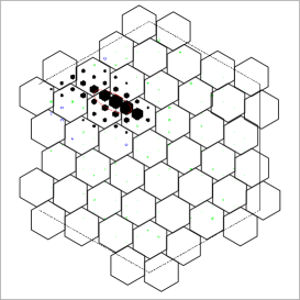
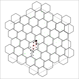
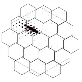
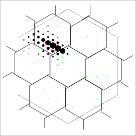
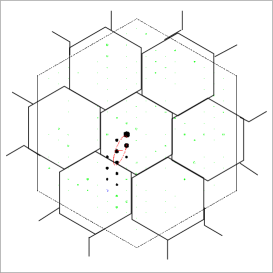
Figure 1: Definition of the cells of pixels for $\ell=2$ (top row), $\ell=3$ (middle row) and $\ell=4$ (bottom row), superimposed to a shower image containing about 2000 photoelectrons (left column) and about 100 photoelectrons (right column). The cells corresponding to $\ell=1$ are the individual pixels. The ampitude in a given pixel is indicated by the block area. The thin line indicates the border of the camera.

Another complication arises from the noise contributions. There is a finite probability to have a very small signal in a pixel, which would make moments with negative index $q$ diverge. Since the amplitude distribution is more or less continuous - the peaks corresponding to 0, 1, 2, … photoelectrons are not resolved individually - such pixels could only be removed by a more or less arbitrary cut. Instead, it was decided to limit the analysis to positive values of $q$, in the range from 2 to 8. The values $q=0$ and $q=1$ yield trivial results; $q=0$ simply counts the numbers of cells and the moment for $q=1$ simply reflects the normalization of the amplitudes.

3 Results

The analysis methods described above were applied to a subset of the data resulting from the observation of the active galaxy Mkn 501 in a high state of activity in the course of the year 1997 ([4], [5]). The data were taken at zenith angles between $10^{\circ}$ and $26^{\circ}$. During these observations, the source was displaced by $0.5^{\circ}$ in declination with respect to the optical axis of the telescopes; a region displaced by the same amount in the opposite region served to evaluate backgrounds under the signal. The sign of the displacement varied between 20-minute runs, in order minimize systematic effects. The distance of $1^{\circ}$ between the signal region and the background region is large enough that events reconstructed stereoscopically can be assigned unambiguosly.

After a preselection keeping only events with shower axes within $0.5^{\circ}$ from the source or from the center of the background region, the data set contained approximately 29.000 events originating from the region centered on the source position opposed to 25.000 hadronic background events. Images showing a total amplitude of more than 40 photoelectrons were included in the analysis.

3.1 Distributions

Figure 2 shows the distributions of the multifractal parameters $\tau_{2}$ and $\alpha_{2}$ for $\gamma$-rays as well as for cosmic rays. The distribution is very well described by a Gaussian function. The multifractal parameter $\tau$ indicates how fast the number of cells of pixels that carry a significant amount of the total amplitude increases, if the size of the cell is decreased. Images originating from a $\gamma$-ray yield smaller values for $\tau$, because these images are well contained in a narrow region of the camera in contrast to the fuzzy images produced by hadronic showers. For these hadronic images, one observes a fast increase in the number of cells with decreasing cell size, and therefore the $\tau$-distribution peaks at larger values.

Figure 2: The distributions of the mass exponent $\tau_{2}$ (left) and the singularity exponent $\alpha_{2}$ (right) for $\gamma$-rays (open circles) und hadrons (filled circles).

The parameter $\alpha$ indicates how fast $\tau$ changes with increasing order $q$. Considering the images of a hadronic shower, they are spread out over a large region of the camera and thus the different cells of pixels carry only small amplitudes, i.e. numbers close to zero in contrast to a $\gamma$-induced shower, which generates amplitudes that are relatively large in the various cells of pixels. With increasing q the moments $Z_{q}(\ell)$ decrease rapidly in the case of images produced by hadrons, resulting in a fast increase in the slope $\tau(q)$ with growing order $q$.

The distribution of the wavelet parameter $\beta_{2}$ is shown in Figure 3. Images of hadronic origin show larger fluctuations on the short length scales compared to an image produced by $\gamma$-rays, that may in fact be described by a smooth gaussian distribution. This results in an increase of the wavelet moments $W_{q}(\ell)$ with decreasing length scale. Therefore, the parameter $\beta$ assumes larger values for hadronic events compared to $\gamma$-rays.

Figure 3: The distribution of the wavelet parameter $\beta_{2}$ for $\gamma$-rays (open circles) and hadrons (filled circles).

3.2 Separation Properties Compared with the Hillas-Parameters

In order to describe the effectiveness of the different parameters with respect to distinguishing between $\gamma$-rays and the hadronic background, cuts on these parameters were applied. From that, efficiencies $\kappa$ and $Q$-values were derived: $\kappa_{\gamma}=N_{\gamma}^{\mbox{\it\scriptsize(cut)}}/N_{\gamma}$, $\kappa_{\mbox{\scriptsize{Hadron}}}=N_{\mbox{\scriptsize{Hadron}}}^{\mbox{\it\scriptsize(cut)}}/N_{\mbox{\scriptsize{Hadron}}}$ and $Q=\kappa_{\gamma}/\sqrt{\kappa_{\mbox{\scriptsize{Hadron}}}}$. The number $N_{\gamma}$ was determined by statistically subtracting the numbers of the events in the source region and in the background region. The $Q$-value describes by how much the significance of a weak signal, calculated as in [15], is enhanced by the cuts. The analysis was first applied to all telescopes individually.

Table 1 lists mean values and standard deviations of the distribution for conventional and multifractal image parameters for the $\gamma$-rays as well as for the hadron-distributions, the $\gamma$-efficiencies $\kappa_{\gamma}$, hadron-efficiencies $\kappa_{\mbox{\scriptsize{Hadron}}}$ and $Q$-values for a cut that yields the largest $Q$-value in descending order with respect to the $Q$-value they archieve. As already evident from Figure 2, multifractal parameters can be employed to enhance the significance of $\gamma$-ray signals, but seem not to be competitive with the conventional parameter scaled width.

	scaled width	$\tau_{2}$	$\alpha_{2}$	scaled length	$\beta_{2}$
$\langle x^{\gamma}\rangle$	1.04	1.18	1.12	0.99	1.45
$\sigma^{\gamma}_{x}$	0.18	0.24	0.24	1.26	0.50
$\langle x^{\mbox{\scriptsize{Hadron}}}\rangle$	1.58	1.47	1.40	0.19	1.81
$\sigma^{\mbox{\scriptsize{Hadron}}}_{x}$	0.38	0.24	0.26	0.29	0.56
$\mbox{{\it cut}}^{\mbox{\it{\scriptsize{(opt)}}}}$	$sw\leq 1.1$	$\tau_{2}\leq 1.25$	$\alpha_{2}\leq 1.25$	$sl\leq 1.2$	$\beta_{2}\leq 1.9$
$\kappa_{\gamma}$	$0.663\pm 0.044$	$0.722\pm 0.050$	$0.797\pm 0.056$	$0.710\pm 0.006$	$0.879\pm 0.067$
$\kappa_{\mbox{\scriptsize{Hadron}}}$	$0.113\pm 0.004$	$0.241\pm 0.005$	$0.338\pm 0.006$	$0.404\pm 0.054$	$0.635\pm 0.008$
Q-value	$1.82\pm 0.12$	$1.47\pm 0.19$	$1.37\pm 0.09$	$1.12\pm 0.08$	$1.10\pm 0.08$

Table 1: Description of the distributions of the various parameters, including efficiencies and the $Q$-value for an optimal cut, i.e. for maximum enhancement of significance. The values quoted refer to events detected with the telescope $\mbox{CT}_{3}$; values resulting from the analysis of images in the other telescopes are consistent within statistics.

3.3 Dependence on $q$

An interesting point is the dependence of the parameters on the index $q$, especially how the separation performance of the parameters is influenced by different weighting exponents. Figure 4 illustrates how the parameters $\tau$ and $\alpha$ change with $q$. Depicted are the mean values for the $\gamma$-ray and hadron distributions a well as their widths resulting from a Gaussian fit.

Figure 4: Mean values and standard deviations of the multifractal parameters $\tau$ (left) and $\alpha$ (right) as a function of the index $q$ for $\gamma$-rays (open circles) and hadrons (filled circles).

The parameters show the expected dependence on $q$. However, their separation performance is virtually unaffected by a particular choice of $q$ – in all cases, the separation between $\gamma$-rays and hadrons corresponds roughly to the width of the distributions. The reason is that parameters of different order $q$ turn out to be strongly correlated.

Furthermore, the values of the multifractal parameters are affected by the position of the shower image relative to the pixel cells, clearly an effect of the relatively large cells. The value of the moment $Z_{q}(\ell)$ depends on the position of the image relative cells of pixels especially for the largest cell. Also the points in the double-logarithmic plot of $Z_{q}(\ell)$ against $\ell$ do not lie on a line as expected from equation 2, but rather on a concave curve. For that reason the slope $\tau$ of a line through these points gets steeper if one includes only the moments $Z_{q}(\ell)$ on the short length scales.

3.4 Correlations

An interesting question is to which extent the multifractal parameters and the Hillas parameters are correlated. If multifractal parameters are genuinely sensitive to fluctations within the image, a weak correlation would be expected. If, on the other hand, the multifractal parameters merely provide a different parametrization of the global shape of the image, one would expect strong correlations.

In Figure 5 the correlation between the multifractal parameter $\tau$ and the Hillas-parameters scaled width and concentration is depicted for the hadronic background. The mean value and the standard deviation of the Hillas parameter is plotted as a function of the value of a multifractal parameter.

Figure 5: Correlation of the multifractal parameter $\tau$ with the Hillas-parameters scaled width (left) and concentration (right).

Clearly, the parameters are not independent of each other. The correlation of the multifractal parameter $\tau$ with scaled width directly follows from the arguments outlined in section 3.1. Furthermore, the correlation of $\tau$ with concentration shows an accumulation of $\gamma$-candidates at small values for $\tau$ and large values for concentration, whereas hadron-candidates amass at large values for $\tau$ and small values for concentration.

3.5 Averaging over Multiple Telescopes

In the conventional analysis using the (scaled) Hillas parameters, separation properties are enhanced by averaging over the images taken from the same shower by the different telescopes. The same is true for the multifractal parameters. Averaging values of the multifractal parameters $\tau$ or $\alpha$ over all telescopes that have been triggered by a given event results in a significant improvement of its separation properties, as can be seen in Table 2. Still, however, are the multifractal parameters inferior in their performance.

	cut	$\kappa_{\gamma}$	$\kappa_{\mbox{\scriptsize{Hadron}}}$	$Q$-value
$\tau_{2}$	$\tau_{2}\leq 1.17$	$0.555\pm 0.035$	$0.076\pm 0.003$	$2.02\pm 0.13$
$\beta_{2}$	$\beta_{2}\leq 1.60$	$0.650\pm 0.046$	$0.318\pm 0.005$	$1.15\pm 0.08$
mean scaled width	$\mbox{\it msw}\leq 1.10$	$0.718\pm 0.043$	$0.074\pm 0.003$	$2.64\pm 0.16$
mean scaled length	$\mbox{\it msl}\leq 1.10$	$0.724\pm 0.039$	$0.326\pm 0.005$	$1.27\pm 0.09$

Table 2: Efficiencies and $Q$-values for an optimal cut for the averaged parameters.

4 Neural Networks

In order to investigate how the $\gamma$/hadron-separation may be improved in spite of the close correlation of the parameters, a neural network was employed. A detailed introduction to the functionality and theory of neural nets may be found in [16]. The analysis was applied to data from individual telescopes. Neural networks of the type ‘feed-forward perceptron’ having

1. the Hillas-parameters width, length, concentration and $\log(\mbox{\it size})$;

2. multifractal and wavelet parameter $\tau_{2}$, $\tau_{4}$, $\tau_{8}$, $\beta_{2}$, $\beta_{4}$, $\beta_{8}$ and $\log(\mbox{\it size})$;

3. all of the above parameters

as input values were implemented and their classification performance was examined. The adjustment of the net’s weights and thresholds was done using a data sample consisting of 1200 events with a reconstructed shower direction within a circle of $0.2^{\circ}$ around the source-position as $\gamma$-rays and 1200 events of background data as hadrons. The events were requested to have an image-size of at least 40 photoelectrons. The network was adjusted in such a way that it produced an output value of $z=0$ for the $\gamma$-candidates and $z=1$ for the hadron-candidates, respectively.

The neural nets were implemented using the JetNet-programme ([17]), that provides a number of interesting features for optimizing the adjusting process such as adding momentum or introducing artificial noise, in order to prevent the system from being trapped in a local minimum. The topology of the network was chosen in such a way that the networks consisted of three layers in all three cases, but the number of nodes within a layer was altered until the net yielded the best result on the training data.

Figure 6 illustrates the distribution of the output $z$ of the neural network, clearly showing an excess of events with low values for $z$ corresponding to $\gamma$-rays.

Figure 6: The distribution of the output $z$ of the neural net using Hillas- as well as multifractal parameters; filled circles correspond to the hadronic background, open circles to $\gamma$-rays. Both distributions have been normalized to unit area.

	cut	$\kappa_{\gamma}$	$\kappa_{\mbox{\scriptsize Hadron}}$	$Q$-value
1.	$z\leq 0.38$	$0.70\pm 0.05$	$0.15\pm 0.004$	$1.79\pm 0.12$
2.	$z\leq 0.34$	$0.54\pm 0.04$	$0.12\pm 0.003$	$1.59\pm 0.11$
3.	$z\leq 0.26$	$0.54\pm 0.05$	$0.07\pm 0.003$	$2.01\pm 0.14$

Table 3: Efficiencies and Q-values for optimal cuts on the neural net output $z$, comparing the various approaches.

The network based on Hillas-parameters was able to reach the performance of the parameter scaled width, that attains a $Q$-value of $1.82\pm 0.12$. The network using all available parameters slightly surpasses the performance of the network that relied on Hillas-parameters. The network based on multifractal and wavelet parameters falls behind, as can be seen from Table 3.

5 Concluding Remarks

Image analysis techniques based on multifractals and wavelets were applied to images recorded by the HEGRA-Čerenkov-telescopes. A $\gamma$/hadron-separation by cuts on these parameters is feasible, yielding a performance similar to the Hillas-parameter concentration, but falling behind that of the parameter scaled width. Combining Hillas parameters and multifractal parameters using a neural network, a slight improvement in performance could be achieved compared to the Hillas parameters alone. The gain is, however, limited by the strong correlation between the Hillas parameters and the multifractal parameters.

A general – and not too surprising – conclusion is certainly that the pixel size of the HEGRA cameras is much too coarse to effectively characterize the fractal nature of showers images; rather than exploring the fine structure of the image, the multifractal parameters determine its overall shape, explaining the good correlation with the Hillas parameter concentration.

Our overall assessment concerning the use of multifractal parameters to identifiy the primary particle of an air shower is less optimistic than the view given in ([9]), in which the analysis method is applied to Monte-Carlo data from a simulation of the TACTIC-experiment. While the pixel size of HEGRA ($0.25^{\circ}$) and TACTIC ($0.31^{\circ}$) are similar, some basic differences between the two analysis should be emphasized:

• The square-grid pixel arrangement of TACTIC simplifies the subdivision into pixel cells.

• The analysis of [9] is applied to images containing at least 1800 photoelectrons, whereas the HEGRA analysis was applied to images with as little as 40 photoelectrons. For such small numbers of photoelectrons, fluctuations in the image are dominated by photoelectron statistics, rather than the shower substructures. For gamma-hadron separation, algorithms which work only for very large images are of limited interest. The situation differs if one applies the technique to separate primary nuclei, which is the main emphasis of [9].

• The analysis of [9] also included multifractal moments for negative exponents $q$. This was possible since in the simulation Poisson-distributed background photoelectrons were added and there is a clear distinction between 0 and 1 photoelectron in a pixel. In HEGRA, with a Gaussian noise of about 1 photoelectron rms, an ad-hoc cut would have to be used to exclude low amplitudes; to avoid this, only positive values of $q$ were allowed.

In order to really judge if one can detected the fractal structure of air showers in their Čerenkov images, one should probably employ a simulation with very fine pixels – such that the first set of length scales is well contained within the image – and a photoelectron yield such that Poisson fluctuations are small compared to the shower fluctuations. The first condition implies a pixel size around $0.002^{\circ}$ to $0.01^{\circ}$, the second an image size of 10000 to 100000 photoelectrons.

References

- [1] T.C. Weekes, Space Science Rev. 75 (1996) 1
- [2] M.F. Cawley and T.C. Weekes, Experimental Astronomy 6 (1996) 7
- [3] A. Konopelko et al., Astroparticle Physics 10 (1999) 275
- [4] F.A. Aharonian et al., Astronomy and Astrophysics 342, 69 (1999)
- [5] F.A. Aharonian et al., Astronomy and Astrophysics 349, 11 (1999)
- [6] A.M. Hillas, Proc. 19th ICRC (La Jolla) 3 445
- [7] D.J. Fegan, J.Phys.G 23 (1997) 1013-1060
- [8] F.A. Aharonian et al., Astronomy and Astrophysics 327, L5 (1997)
- [9] A. Haungs et al., Astroparticle Physics 11 (1999) 145
- [10] J. Feder, Fractals, Plenum Press, New York, 1988
- [11] E. Bacry et al., J. Stat. Phys. 70 (1993) 635
- [12] J.W. Kantelhardt et al., Physica A 220 (1995) 219-238
- [13] F.A. Aharonian, Proceedings of the Int. Workshop “Towards a Major Atmospheric Čerenkov Detector II”, Calgary, (1993), R.C. Lamb (Ed.), p. 81.
- [14] G. Hermann, Proceedings of the Int. Workshop “Towards a Major Atmospheric Čerenkov Detector IV”, Padua, (1995), M. Cresti (Ed.), p. 396
- [15] T.P. Li, Y.Q. Ma, Astrophysical Journal, 272: 317-324, 1983
- [16] R. Beale, T. Jackson, Neural Computing, IOP, London, 1992
- [17] L. Lönnblad et al., Comp. Phys. Comm. 70 (1992) 167-182