The spatial distribution of O-B5 stars in the solar neighborhood as measured by Hipparcos

Abstract

We have developed a method to calculate the fundamental parameters of the vertical structure of the Galaxy in the solar neighborhood from trigonometric parallaxes alone. The method takes into account Lutz-Kelker-type biases in a self-consistent way and has been applied to a sample of O-B5 stars obtained from the Hipparcos catalog. We find that the Sun is located 24.2 $\pm$ 1.7 (random) $\pm$ 0.4 (systematic) pc above the galactic plane and that the disk O-B5 stellar population is distributed with a scale height of 34.2 $\pm$ 0.8 (random) $\pm$ 2.5 (systematic) pc and an integrated surface density of (1.62 $\pm$ 0.04 (random) $\pm$ 0.14 (systematic)$)\cdot 10^{-3}$ stars pc^-2. A halo component is also detected in the distribution and constitutes at least $\approx 5$% of the total O-B5 population. The O-B5 stellar population within $\sim 100$ pc of the Sun has an anomalous spatial distribution, with a less-than-average number density. This local disturbance is probably associated with the expansion of Gould’s belt.

1 INTRODUCTION

Studies based on the spatial distribution of massive stars (Blaauw, 1960) and interstellar hydrogen (Gum et al., 1960) established some time ago that the Sun is located above the galactic plane. This has been confirmed using a variety of tracers (see Humphreys & Larsen 1995 for a review) with somewhat incompatible values of $z_{\sun}$, the Sun’s distance above the galactic plane, ranging from 9.5 pc to 42 pc. Some of the discrepancies may be due to real differences in the vertical distribution of different stellar or gaseous components but others must be due to observational errors, since they appear among studies of the same type of objects. This is seen in Table 1, where the results on early-type stars are shown. The use of early-type stars to determine $z_{\sun}$ has the advantage that their scale height with respect to the galactic plane, $h$, is of the same order of magnitude as $z_{\sun}$, which makes the determination simpler than for objects with larger scale heights (e.g. late-type stars). However, early-type stars are scarce and to obtain a statistically-reliable sample previous studies had to resort to objects close to the galactic plane, where extinction can introduce severe biases.

The measurement of $z_{\sun}$ using early-type stars is closely related to the vertical distribution of the number density of those stars, $\rho(z)$. We consider here two scenarios. First, if the analyzed sample consists of a single population which is responsible for the gravity field in which the stars are moving we have a a single component, self-gravitating, isothermal disk (e.g. King 1996), which can be described by:

$$\rho(z)=\mbox{$\rho_{\rm o}$}\,{\rm sech}^{2}\left(\frac{z+\mbox{$z_{\sun}$}}{2h_{s}}\right),$$ (1)

where $z$ is the vertical coordinate (with its origin at the Sun’s position), $h_{s}$ is the corresponding scale height, and $\rho_{\rm o}$ is the density at the galactic plane. The factor of 2 is introduced in order to have $\rho\propto\exp(-|z+\mbox{$z_{\sun}$}|/h_{s})$ for $|z+\mbox{$z_{\sun}$}|\gg h_{s}$. A second possible scenario can be introduced by assuming the same conditions as before but now establishing that the gravity field is caused by a different population (e.g. low-mass stars or dark matter) with constant density. In that case we have a Gaussian vertical distribution:

$$\rho(z)=\mbox{$\rho_{\rm o}$}\,\exp\left(-\frac{1}{2}\left(\frac{z+\mbox{$z_{\sun}$}}{h_{g}}\right)^{2}\right),$$ (2)

where $h_{g}$ is the Gaussian half-width.

The stellar surface density, $\sigma_{\star}$, can be obtained by integrating $\rho(z)$ from $-\infty$ to $+\infty$ and for the models described by Eqs. 1 and 2 the results are $4h_{s}\mbox{$\rho_{\rm o}$}$ and $\sqrt{2\pi}h_{g}\mbox{$\rho_{\rm o}$}$, respectively. Measured values of $h$ and $\sigma_{\star}$ have been included in Table 1. In each case it is indicated whether the model used is that of Eq. 1 or an exponential one: $\rho(z)=\mbox{$\rho_{\rm o}$}\,\exp(-|z+\mbox{$z_{\sun}$}|/h_{e})$, in which case $\sigma_{\star}=2h_{e}\mbox{$\rho_{\rm o}$}$.

Table 1: Previous determinations of parameters associated with the vertical distribution of the early-type stellar population. The last column was calculated by multiplying the measured surface density by a factor derived from an unbiased O+B sample.

Source	$h$	$z_{\sun}$	Range	Model	$\sigma_{\star,\,\rm meas}$	Range	$\sigma_{\star,\,\rm equiv}$
	(pc)	(pc)			(stars pc-2)		(stars pc-2)
Allen (1973)	60	—–	O+B	exponential	$1.2\cdot 10^{-2}$	O+B	$2.6\cdot 10^{-3}$
Stothers & Frogel (1974)	$46\pm 7$	$\;24\pm 3$	O-B5	exponential	$5.3\cdot 10^{-4}$	O-B3.5	$0.85\cdot 10^{-3}$
	$70\pm 3$
Conti & Vacca (1990)	$45\pm 5$	$\;15\pm 3$	WR	self-gravitating	—–	—–	—–
Reed (1997, 2000)	$45\pm 20$	$9.5\pm 3.5$	O-B2	exponential	$(0.6-8.0)\cdot 10^{-4}$	O-B2	$(0.15-1.95)\cdot 10^{-3}$

The profiles defined by Eqs. 1 or 2 are actually not extremely different from one another and either one of them is expected to be a reasonably good approximation to the vertical profile of the disk population of early-type stars. However, we must bear in mind that there are also early-type stars in the halo (see, e.g. Rolleston et al. 1999 and references therein) which are expected to dominate the O-B5 population at distances larger than several hundred pc from the galactic plane and, thus, add another component to the observed disk population. Most of these objects are runaway stars (Rolleston et al., 1999; Hoogerwerf et al., 2000) but some appear to have been formed in situ (Conlon et al., 1992).

The availability of the Hipparcos catalog (ESA, 1997) has revolutionized the quality of astrometric data and has produced for the first time good-quality trigonometric parallaxes for a large sample of early-type stars. However, even with these data one has to take into account a fundamental problem in the use of trigonometric parallaxes for the determination of distances discovered by Lutz & Kelker (1973). Assuming a uniform spatial distribution of stars and a Gaussian distribution of observed parallaxes $\pi_{\rm o}$ about the true parallax $\pi$ with a width $\sigma_{\pi}$, they discovered that the distribution of true distances $r=1/\pi$ about the observed one $\mbox{$r_{\rm o}$}=1/\mbox{$\pi_{\rm o}$}$ was asymmetrical and even divergent for $r\rightarrow\infty$. The effect is caused by the inverse relationship between $\pi$ and $r$ and by the fact that the available volume between $r$ and $r+dr$ is proportional to $r^{2}$. The effect is unimportant for parallaxes with small relative errors ($\varepsilon_{\pi}\equiv\sigma_{\pi}/\mbox{$\pi_{\rm o}$}\lesssim 0.05$) and can be corrected for cases with $\varepsilon_{\pi}\approx 0.10-0.15$ but for values with $\varepsilon_{\pi}\gtrsim 0.175$ it becomes so large that an individual trigonometric parallax by itself provides little information about the distance to the object unless it is combined with additional information (e.g. the spectroscopic parallax). Lutz & Kelker (1973) provided a table to correct the effect of the bias for $\varepsilon_{\pi}<0.175$ (see Smith (1987); Kovalevsky (1998) for updated analyses) but for larger values no simple meaningful correction exists.

A large fraction of the Hipparcos trigonometric parallaxes have $\varepsilon_{\pi}>0.175$ and a non-negligible number have negative parallaxes. Those values cannot be discarded when statistical studies of distances are undertaken without introducing severe biases. One approach to the problem is that of Ratnatunga & Casertano (1991), who use spectroscopic parallaxes to constrain the possible range of distances without discarding any stars with large values of $\varepsilon_{\pi}$ or negative ones of $\pi_{\rm o}$. Another approach is that followed by Feast & Catchpole (1997) to evaluate the zero-point of the Cepheid period-luminosity relation. Those authors combine trigonometric parallaxes with $\varepsilon_{\pi}$ up to $\approx 1.0$ with the apparent magnitude and period of the stars to reduce all Cepheids to a single distance and produce an equivalent parallax with $\varepsilon_{\pi}\approx 0.05$.

In this paper we introduce a new method to correct for Lutz-Kelker-type biases (section 2) and apply it to a sample of stars obtained from the Hipparcos catalog (section 3) in order to derive the parameters which determine the vertical distribution of O-B5 stars in the solar neighborhood (section 4).

2 DESCRIPTION OF THE METHOD

The number of stars per unit distance $n_{\star,r}$ between $r$ and $r+dr$ inside a solid angle $\Omega$, $n_{\star,r}dr$, is given by:

$$n_{\star,r}dr=\rho(r)\,\Omega\,r^{2}\,dr,$$ (3)

where $\rho(r)$ is the star number density. The equivalent expression per unit parallax is:

$$n_{\star,\pi}d\pi=\rho(1/\pi)\,\Omega\,\pi\mbox{${}^{-4}$}\,d\pi.$$ (4)

If we assume that the distribution of $\pi_{\rm o}$ about $\pi$ is Gaussian with a width $\sigma_{\pi}$, then the distribution of observed parallaxes will be the convolution of the two functions:

$$f(\mbox{$\pi_{\rm o}$})=\int_{0}^{\infty}A\,e^{-\frac{1}{2}\left(\frac{\pi-\pi_{\rm o}}{\sigma_{\pi}}\right)^{2}}\rho(1/\pi)\,\Omega\,\pi\mbox{${}^{-4}$}\,d\pi,$$ (5)

where $A$ is a normalizing factor. Note that Eq. 4 may be singular at $\pi=0$ for some choices of $\rho(r)$ and that this may cause Eq. 5 to be non-normalizable. This is the reason why no simple correction can be obtained for the standard case of Lutz-Kelker bias (which has $\rho(r)=\mbox{$\rho_{\rm o}$}$) when $\varepsilon_{\pi}\gtrsim 0.175$. A generalization of that standard case can be achieved by allowing for non-constant density profiles, as previously suggested by Hanson (1979). This is motivated by the finite size of the Galaxy, which forces the introduction of a cutoff in any choice of $\rho(r)$ based on a realistic model. Such a cutoff would eliminate any convergence problems in Eq. 5 and allow for finite Lutz-Kelker-type corrections.

We consider one such model based on a self-gravitating isothermal vertical distribution (Eq. 1) and which for early-type stars should be valid for large absolute values of the galactic latitude $b$, where the main limitation imposed on sample completeness is distance (as opposed to extinction):

$$\rho(1/\pi)=\mbox{$\rho_{\rm o}$}\,{\rm sech}^{2}\left(\frac{\sin b/\pi+\mbox{$z_{\sun}$}}{2h_{s}}\right)=\mbox{$\rho_{\rm o}$}\,{\rm sech}^{2}\left(\frac{1/\pi\pm\mbox{$z_{\sun}$}^{\prime}}{2h_{s}^{\prime}}\right),$$ (6)

where $h_{s}^{\prime}=h_{s}\,|\csc b|$ and $z_{\sun}$${}^{\prime}=\mbox{$z_{\sun}$}\,|\csc b|$, and the sign in the last expression is positive for $b>0$ and negative for $b<0$. A least-squares fit to the observed distribution of parallaxes using Eqs. 5 and 6 should then yield the three free parameters $h_{s}$, $z_{\sun}$, and $\sigma_{\star}$ (which is a function of the constants in the two equations). Unfortunately, two problems exist when this is attempted. First, a large range in $b$ needs to be used in order to have a large enough sample, which implies that a mean value of $|\csc b|$ will have to be obtained in order to derive $h_{s}$ and $z_{\sun}$ from $h_{s}^{\prime}$ and $z_{\sun}$^′. However, for $|b|\lesssim 25\arcdeg$ and reasonable values of $h_{s}$ and $z_{\sun}$, $|\csc b|$ becomes so large that we are forced to go to distances larger than 1 kpc in order to have reasonably complete samples, and this is beyond the volume well-sampled by Hipparcos. Therefore, this method cannot be applied to the data currently available. The second problem is more subtle: Suppose we analyze all the stars contained within a double cone defined by $|b|>b_{\rm min}$ and that the vertical spatial distribution of early-type stars is given by the sum of either Eq. 1 or Eq. 2 and a halo component which is unimportant near the galactic plane but dominates at high $|z|$. Then, since the sampled volume is proportional to $z^{2}$, the halo component will be overrepresented in our sample and a strong bias could be introduced in our measurements of $h_{s}$ and $z_{\sun}$ unless the proper linear combination of $\rho_{\rm disk}$ and $\rho_{\rm halo}$ is used.

An alternative method which avoids these two problems can be designed in the following way. Suppose we can make an educated guess for the parameters that describe the O-B5 disk population (using either Eq. 1 or Eq. 2) and that we also have a reasonably good approximation for the halo population (which is expected to be only a small contaminant in our sample if we avoid the bias mentioned in the previous paragraph). Then, for a single star with measured $\pi_{\rm o}$, $\sigma_{\pi}$, and $b$ we can calculate the probability distribution as a function of distance as:

$$p(r)=A\,r^{2}\,e^{-\frac{1}{2}\left(\frac{1-r\pi_{\rm o}}{r\sigma_{\pi}}\right)^{2}}\rho(r),$$ (7)

where $A$ is a normalizing factor and the latitude dependence is embedded in $\rho(r)=\rho_{\rm disk}(r)+\rho_{\rm halo}(r)$. We can now project $p(r)$ into the vertical coordinate to obtain $p(z)$ and sum over all observed stars to obtain $f(z)$, the distribution of stars as a function of the vertical coordinate. Doing a least-squares fit of $f(z)$ with a vertical profile leads to a new estimate of the parameters. The process is then repeated until convergence is achieved.

Several precautions have to be taken to insure the correctness of this iterative process. First, a maximum distance to the Sun vertical line, $\varpi_{\rm max}$, has to be specified in order to insure completeness and to avoid the halo-disk bias previuosly discussed. This can be achieved by truncating each individual $f(z)$ at $z_{\rm max}=\varpi_{\rm max}\tan b$. Second, stars at very low galactic latitudes ($|b|<b_{\rm min}$) have to be excluded from the sample since for lines of sight close to the galactic equator the spatial structure is dominated by radial (not vertical) variations and extinction. In order not to induce any biases due to this exclusion, the fit to the vertical profile should not include the range $(-\varpi_{\rm max}\tan b_{\rm min},\varpi_{\rm max}\tan b_{\rm min})$. As shown in Fig. 1, the resulting volume which will be used for our fit to the vertical profile is a double semi-infinite cylinder. For any given star with $|b|>b_{\rm min}$, three regions are then defined: $0<|z|<\varpi_{\rm max}\tan b_{\rm min}$, $\varpi_{\rm max}\tan b_{\rm min}\leq|z|\leq\varpi_{\rm max}\tan|b|$, and $\varpi_{\rm max}\tan|b|<|z|<\infty$, and only the second one is used for our calculation. A star with a large value of $\varepsilon_{\pi}$ will have non-negligible values of $f(z)$ in the three regions while the probability distribution for one with a small value of $\varepsilon_{\pi}$ will be concentrated in one of the three (unless its value of $\pi_{\rm o}$ is close to one of the two critical values which correspond to the two boundaries between regions). In any case, each of those stars will have an integrated probability in the second region between 0 and 1, leading to a non-integral estimated number of stars in the double semi-infinite cylinder. A third precaution to be considered is the introduction of biases in the obtained parameters by the fitting procedure. This problem can be solved using a twofold strategy: First, biases can be minimized using a variable bin size determined by the criteria specified by D’Agostino & Stephens (1986). Second, a population with the same parameters as those derived in the fitting process can be generated numerically and fitted using the same procedure. Repeating this a large number of times allows us to measure the numerical biases by obtaining the mean displacements between the real and the derived parameters and to correct our results accordingly.

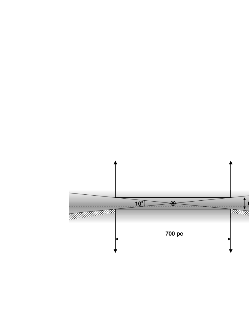
Figure 1: The double semi-infinite cylinder used in this paper to study the vertical distribution of O-B5 stars is represented by the two regions contained inside the thick lines. The values of the parameters used are $\varpi_{\rm max}=350$ pc and $b_{\rm min}=5\arcdeg$. The shaded area represents the galactic disk with the dashed line being the galactic plane and the Sun symbol marking the position of our star. The hatched regions mark the area excluded to estimate the bias induced by extinction (see the text for details).

3 THE SAMPLE

We have extracted from the Hipparcos catalog the data for all stars classified therein as O-B5 and with $|b|>b_{\rm min}=5\arcdeg$ (3 531 objects). That value of $b_{\rm min}$ was chosen in order to eliminate the highly obscured regions near the galactic plane while at the same time retaining most of the O-B5 stars in the immediate solar neighborhood. Also, for $h\approx 45$ pc (a typical value chosen from Table 1), a vertical distance of three scale heights corresponds to $\approx 1.5$ kpc in $\varpi$ for $|b|=5\arcdeg$, so we would not expect to sample regions with large variations in the early-type star population due to radial galactic gradients. From that sample we have selected a subsample (3 382 objects) with good astrometric solutions by eliminating those stars with more than 5% or data points rejected (column 29, ESA 1997) and with a goodness-of-fit statistic $g$ for $\nu$ degrees of freedom:

$$g=\left(\frac{9\nu}{2}\right)^{1/2}\left[\left(\frac{\chi^{2}}{\nu}\right)^{1/3}+\frac{2}{9\nu}-1\right],$$ (8)

less than 3.0 (column 30)

Since we expect most stars in our subsample to be located at distances $>100$ pc and that for Hipparcos data, typically, $\sigma_{\pi}\approx 1$ mas, Lutz-Kelker-type biases should be important. Indeed, that is what can be deduced from Table 2, where the distribution of $\varepsilon_{\pi}$ values is shown.

Table 2: Frequency of Hipparcos relative parallax errors for the selected subsample of 3  382 O-B5 stars used in this work. The last row refers to stars with negative parallaxes.

$\varepsilon_{\pi}$ range	Number
$0.00-0.05$	6
$0.05-0.15$	237
$0.15-0.25$	380
$0.25-0.50$	848
$>0.50$	1 444
negative	467

The other parameter which has to be selected to define the double semi-infinite cylinder which will be used in this work is $\varpi_{\rm max}$. To do that, we have to consider that the Hipparcos completeness limit for early-type stars is determined by $m_{V}=7.9+1.1|\sin b|$, which corresponds to $m_{V}=8.0$ for $|b|=5\arcdeg$. A very small fraction ($\ll 1\%$) of stars below the limit is actually not included and the catalog is partially complete between that limit and $m_{V}\approx 12-13$ (ESA, 1997). A B5 V star has $M_{V}\approx-1.2$; at a distance of 350 pc such a star with $A_{V}=1.0$ mag (obtained from a very conservative estimate of 3.0 mag/kpc in $V$) would have $m_{V}=7.5$, still within the completeness limit. If such a star was located at 135 pc (approximately 3 scale heights) from the galactic plane and with $\varpi=350$ pc, its apparent magnitude would also be $\approx 7.5$ if we estimate $A_{V}$ as $\approx 0.5$ (again, a very conservative estimate at that latitude). We can then conclude that a choice of $\varpi_{\rm max}=350$ pc leads to a nearly complete sample for the O-B5 disk stellar population.

4 RESULTS

We have carried out least-squares fits to the data described in section 3 using either a self-gravitating isothermal or a Gaussian disk model and applying the method described in section 2. Since the halo population in our sample is clearly incomplete due to the Hipparcos magnitude limits, we used a simple reasonable model to describe it, a parabola. That choice allows us to discriminate between the disk and halo contributions within a few hundred parsecs of the Sun but can only produce a lower limit for $\sigma_{\star,{\rm halo}}$. The data and fits are displayed in Figs. 2 and 3 and the obtained parameters are shown in Table 3.

Figure 2: Observed (histogram) and model fit frequency distributions as a function of the vertical coordinate for O-B5 stars using a self-gravitating isothermal disk + parabolic halo distribution. The dotted lines represent each individual component and the continuous one the sum of the two. The displayed bin size is uniform and equal to 50 pc, but is not used for the fit (see text). The region immediately surrounding $z=0$ is not considered for the fit, as it corresponds to the space between the two semi-infinite cylinders. Note that the observed distribution shows “fractional stars” due to the procedure used to derive the histogram.

Figure 3: Same as Fig. 2 but using a Gaussian disk model instead of a self-gravitating isothermal one.

Table 3: Results of the least-squares fits using either a self-gravitating isothermal (first row) or a Gaussian (second row) disk + parabolic halo distribution. The values have been bias-corrected, and both the random (first) and systematic (second) uncertainties are shown in each case. The $h$ column refers to the scale height ($h_{s}$) in the first row and to the half-width ($h_{g}$) in the second row. No uncertainties are given for $\mbox{$\sigma_{\star,{\rm halo}}$}/\mbox{$\sigma_{\star,{\rm disk}}$}$ because the fitted values are only lower-limits to the real distributions.

Model	$h$	$z_{\sun}$	$\sigma_{\star,{\rm disk}}$	$\mbox{$\sigma_{\star,{\rm halo}}$}/\mbox{$\sigma_{\star,{\rm disk}}$}$	$\chi^{2}/\nu$	$\nu$	$g$
	(pc)	(pc)	(10-3 O-B5 stars pc-2)
1	$34.2\pm 0.8\pm 2.5$	$24.2\pm 1.7\pm 0.4$	$1.62\pm 0.04\pm 0.14$	0.058	0.88	41	$-0.50$
2	$62.8\pm 1.7\pm 4.7$	$25.2\pm 1.5\pm 0.5$	$1.67\pm 0.04\pm 0.24$	0.037	0.87	41	$-0.56$

As previously discussed, a variable bin size was used in order to minimize numerical biases. For each of the two models we generated 50 populations with the same parameters derived from the real population and we estimated the biases by calculating the difference between the mean values of the derived parameters and the real ones. As expected, those biases where very small, typically 0.5 pc for $h$ and $z_{\sun}$. However, one possible bias due to extinction still remains. Suppose we are observing a star with $b=-5\arcdeg$ located inside the double semi-infinite cylinder but with a high value of $\varepsilon_{\pi}$: This star will be counted only as a “fractional star” (i.e. its integrated probability inside the volume of interest will not be close to one). If the sample were complete both inside and outside the double semi-infinite cylinder this would not be a problem, since the lost probability would be compensated by that contributed by stars located outside the cylinder. However, we expect that extinction (and, to a lesser degree, distance) will remove from our sample some of the stars outside the cylinder, especially those closer to the galactic plane. To simulate this effect we consider an extreme case by placing a wall of infinite extinction at $\varpi=\varpi_{\rm max}$ which extends one scale height (for the self-gravitating isothermal case) or one half-width (for the Gaussian case) north and south of the galactic plane. The volume excluded by this wall is represented by the hatched area in Fig. 1 for the self-gravitating isothermal case. Note that only stars in the southern galactic hemisphere are eliminated by this wall since the position of the Sun above the galactic plane locates any star with $b=5\arcdeg$ above the wall. Under these conditions, we eliminated the stars in the hatched volume from our generated 50 populations and calculated the corresponding biases by calculating new least-squares fits. As expected, the new biases turned out to be more relevant than the ones obtained before, but even then they never induced changes larger than 15% in the values of the parameters. Since the real situation must be in between the two extreme cases discussed here ((a) all stars in the possibly excluded area partially contributing to the probability inside the cylinder and (b) none of them doing so), we considered the real bias to be the average of the two and we indicated the two extremes as a systematic error.

The results in Table 3 indicate that both the self-gravitating isothermal and the Gaussian models are very good descriptions of the disk population, since $g$ is close to 0 in both cases and the fitted distribution near the galactic plane closely resembles the observed one, as shown in Figs. 2 and 3. The parabolic fit to the halo population is of worse quality, as expected from the much smaller number of stars in our sample belonging to it and from its incompleteness. Nevertheless, the existence of a halo population in our sample is beyond doubt, as is clearly shown in Figs. 2 and 3. It is also well known that this halo population extends farther than the distance-induced limits in our sample, even beyond a few kpc (Rolleston et al., 1999). Thus, the values of $\mbox{$\sigma_{\star,{\rm halo}}$}/\mbox{$\sigma_{\star,{\rm disk}}$}$ which appear there have to be understood only as lower limits to the real ones.

The values of $z_{\sun}$ and $\sigma_{\star,{\rm disk}}$ obtained using the two different models are clearly compatible. Since we are unable to determine which of the two models provides a better fit to the disk population, either result can be used. Probably the ones obtained with the self-gravitating isothermal profile are preferred due to the better quality of the parabolic fit to the halo population, which should introduce less numerical noise into the result than in the Gaussian case.

Our value for $h_{s}$ is somewhat lower than the ones obtained by other authors. The discrepancies are only at the $2\sigma$ level with the values obtained by Conti & Vacca (1990) and by Stothers & Frogel (1974) (within 200 pc of the Sun) and even lower in comparison with the Reed (2000) result. Allen (1973) does not quote an uncertainty while the value of Stothers & Frogel (1974) within 800 pc of the Sun is quite probably affected by heavy extinction. Some of the discrepancies may be attributed to contamination by halo stars (a non-negligible effect, as we have seen) and others to the use of a purely exponential model instead of a self-gravitating isothermal one. Our value of $z_{\sun}$ is clearly compatible with the one obtained by Stothers & Frogel (1974) but is higher than the ones obtained by Conti & Vacca (1990) and Reed (1997), in this last case by a large amount. We believe that the differences may be caused by the difficulty in accounting for complex extinction variations at low galactic latitudes, especially when one has to rely on spectroscopic parallaxes, a problem which does not affect our results since they are based on unbiased trigonometric distances. This can be seen in the fact that the result more similar to ours is the one which is obtained from the nearest population. Finally, our value for $\sigma_{\star}$ is within the range obtained by Reed (2000) but is clearly higher than the one obtained by Stothers & Frogel (1974) and lower than the one obtained by Allen (1973). Once again, we believe that extinction may be responsible for some of the discrepancies but we must also take into account that $\sigma_{\star}$ is expected to suffer significant variations depending on the maximum radius used, since different regions of the disk (close or far from spiral arms) are expected to be sampled.

One last point to discuss is the existence of spatial variations within the region discussed in this paper. Stothers & Frogel (1974) discovered that a 100 pc radius hole exists in the distribution of O-B5 stars at low galactic latitudes. Also, it has been known for a long time that a large fraction of the early-type stars in the solar neighborhood belong to Gould’s belt, a structure inclined $15-20\arcdeg$ with respect to the galactic plane and which is expanding with respect to a point located close to the Sun’s position (see Torra et al. 2000 for a recent analysis). Is this expected minimum in the number density of early-type stars detected in the Hipparcos data? It indeed is. The parameters derived from our self-gravitating isothermal model predict that there should be 11.6 O-B5 stars within 66.67 pc of the Sun (i.e., with $\pi\geq 15$ mas). However, only three O-B5 stars are found in that volume: $\eta$ UMa, $\alpha$ Eri, and $\alpha$ Pav. The difference between the expected and the measured number appears to be too large to be explained as a statistical fluctuation, so we conclude that the existence of a local “hole” in the distribution of early-type stars is indeed real.

We conclude that our method provides a solid measurement of the vertical distribution of O-B5 stars in the solar neighborhood by using trigonometric parallaxes alone and by taking into account all relevant biases.

References

- Allen (1973) Allen, C. W. 1973, Astrophysical Quantities (Athlone Press)
- Blaauw (1960) Blaauw, A. 1960, MNRAS, 121, 164
- Conlon et al. (1992) Conlon, E. S., Dufton, P. L., Keenan, F. P., McCausland, R. J. H., & Holmgren, D. 1992, ApJ, 400, 273
- Conti & Vacca (1990) Conti, P. S., & Vacca, W. D. 1990, AJ, 100, 431
- D’Agostino & Stephens (1986) D’Agostino, R. B., & Stephens, M. A. 1986, Goodness-of-fit techniques (Marcel-Dekker)
- ESA (1997) ESA. 1997, The Hipparcos and Tycho Catalogues (ESA SP-1200)
- Feast & Catchpole (1997) Feast, M. W., & Catchpole, R. M. 1997, MNRAS, 286, L1
- Gum et al. (1960) Gum, C. S., Kerr, F. J., & Westerhout, G. 1960, MNRAS, 121, 132
- Hanson (1979) Hanson, R. B. 1979, MNRAS, 186, 875
- Hoogerwerf et al. (2000) Hoogerwerf, R., de Bruijne, J. H. J., & de Zeeuw, P. T. 2000, ApJ, 544, 133L
- Humphreys & Larsen (1995) Humphreys, R. M., & Larsen, J. A. 1995, AJ, 110, 2183
- King (1996) King, I. R. 1996, Stellar Dynamics (University Science Books)
- Kovalevsky (1998) Kovalevsky, J. 1998, A&A, 340, L35
- Lutz & Kelker (1973) Lutz, T. E., & Kelker, D. H. 1973, PASP, 85, 573
- Ratnatunga & Casertano (1991) Ratnatunga, K. U., & Casertano, S. 1991, AJ, 101, 1075
- Reed (1997) Reed, B. C. 1997, PASP, 109, 1145
- Reed (2000) Reed, B. C. 2000, AJ, 120, 314
- Rolleston et al. (1999) Rolleston, W. R. J., Hambly, N. C., Keenan, F. P., Dufton, P. L., & Saffer, R. A. 1999, A&A, 347, 69
- Smith (1987) Smith, H., Jr. 1987, A&A, 188, 233
- Stothers & Frogel (1974) Stothers, R., & Frogel, J. A. 1974, AJ, 79, 456
- Torra et al. (2000) Torra, J., Fernández, D., & Figueras, F. 2000, A&A, 359, 82