X-Ray Line Profiles from Parameterized Emission within an Accelerating Stellar Wind

Abstract

Motivated by recent detections by the XMM and Chandra satellites of X-ray line emission from hot, luminous stars, we present synthetic line profiles for X-rays emitted within parameterized models of a hot-star wind. The X-ray line emission is taken to occur at a sharply defined co-moving-frame resonance wavelength, which is Doppler-shifted by a stellar wind outflow parameterized by a ‘beta’ velocity law, $v(r)=v_{\infty}(1-{{R_{\mathchar 8707\relax}}}/r)^{\beta}$. Above some initial onset radius $R_{o}$ for X-ray emission, the radial variation of the emission filling factor is assumed to decline as a power-law in radius, $f(r)\sim r^{-q}$. The computed emission profiles also account for continuum absorption within the wind, with the overall strength characterized by a cumulative optical depth $\tau_{\mathchar 8707\relax}$. In terms of a wavelength shift from line-center scaled in units of the wind terminal speed $v_{\infty}$, we present normalized X-ray line profiles for various combinations of the parameters $\beta$, $\tau_{\mathchar 8707\relax}$, $q$ and $R_{o}$, and including also the effect of instrumental and/or macroturbulent broadening as characterized by a Gaussian with a parameterized width $\sigma$. We discuss the implications for interpreting observed hot-star X-ray spectra, with emphasis on signatures for discriminating between “coronal” and “wind-shock” scenarios. In particular, we note that in profiles observed so far the substantial amount of emission longward of line center will be difficult to reconcile with the expected attenuation by the wind and stellar core in either a wind-shock or coronal model.

1 Introduction

Over the past two decades, orbiting X-ray observatories from Einstein to ASCA have shown that both hot and cool stars are moderately strong sources of soft X-rays at energies betweenm 0.1 and 2 keV. For cooler, late-type stars, the scaling of X-ray luminosity with, e.g., stellar rotation, suggests a solar-type origin, with surface magnetic loops confining hot, X-ray-emitting material within nearly static circumstellar coronae. For hotter, early-type stars, the X-ray luminosity has no discernible dependence on rotation, but instead scales nearly linearly with bolometric luminosity, $L_{\rm x}\approx 10^{-7}L_{\rm Bol}$ (Long & White, 1980; Pallavicini et al., 1981; Chlebowski, Harnden, & Sciortino, 1989), suggesting a different emission mechanism, perhaps related to the high-density, radiatively driven stellar wind observed from such stars.

Nonetheless, an ongoing question has remained whether such hot-star X-ray emission originates from coronal-like processes occuring in nearly static regions near the stellar surface (Cassinelli & Olson, 1979; Waldron, 1984; Cohen, Cassinelli, & MacFarlane, 1997), or rather in the highly supersonic wind outflow, perhaps from shocks arising from intrinsic instabilities in the radiative driving mechanism (Lucy & White, 1980; Lucy, 1982; Owocki, Castor, & Rybicki, 1988; Feldmeier et al., 1997; Feldmeier, Puls, & Pauldrach, 1997; Owocki & Cohen, 1999). Based on the observed strong winds in hot stars (e.g., Snow & Morton, 1976), a key discriminant has been the apparent general lack of soft X-ray absorption, which, along with optical and UV spectral constraints, implies limits to the extent, temperature, and fractional contribution of the total X-ray output from a base corona (Cassinelli, Olson, & Stalio, 1978; Nordsieck, Cassinelli, & Anderson, 1981; Cassinelli & Swank, 1983; Baade & Lucy, 1987; MacFarlane et al., 1993; Cohen et al., 1996). This limited inferred absorption is thus generally seen as evidence for emission arising from lower-density regions at large radii, in general agreement with a wind-shock model.

In the context of extreme ultraviolet spectroscopy, MacFarlane et al. (1991) presented models of emission line profiles, from both a coronal source and from an expanding shell, affected by transfer through a stellar wind. These authors demonstrated that emission line profiles are a key discriminant of the source location. However, due to the small throughput and modest resolution of the Extreme Ultraviolet Explorer (EUVE) spectrometers, combined with the extreme opacity of the interstellar medium in this bandpass, emission lines from only one hot star ($\epsilon$ CMa) were observed with EUVE. The only high signal-to-noise line seen in this EUV spectrum was the He II Ly$\alpha$ line, which was observed to be broadened by several hundred km s^-1, lending credence to models that postulate a wind-origin for the hot plasma in OB stars (Cassinelli et al., 1995).

It is only recently, however, that orbiting X-ray observatories like XMM and Chandra have been able to provide the first detections of spectrally resolved X-ray emission lines from hot, luminous stars (Kahn et al., 2001; Schulz et al., 2001; Waldron & Cassinelli, 2001; Cassinelli et al., 2001). Through the broadened profiles of these resolved X-ray emission lines, these data provide a new, key diagnostic for inferring whether the X-ray emission originates from a nearly static corona, or from an expanding stellar wind outflow. A key goal of the present paper is to provide a firm basis for interpreting such X-ray emission line spectra.

Specifically, we describe below the method (§2) and results (§3) for computations of synthetic line profiles arising from parameterized forms of X-ray emission in an expanding stellar wind. In comparison to recent work by Ignace (2001), who derived analytic forms for X-ray emission profiles for the case of constant expansion velocity, our analysis takes into account a variation of velocity $v(r)$ in radius $r$, as parameterized by the so-called ‘beta-law’ form $v(r)=v_{\infty}(1-{{R_{\mathchar 8707\relax}}}/r)^{\beta}$, where ${{R_{\mathchar 8707\relax}}}$ is the stellar radius and $v_{\infty}$ is the wind terminal speed. As in Ignace (2001), the overall level of attenuation is characterized by an integral optical depth $\tau_{\mathchar 8707\relax}$, and the X-ray emission filling factor is assumed to decline outward as a power law in radius, $f(r)\sim r^{-q}$. However, we also allow for this emission to begin at a specified onset radius $R_{o}$ that can be set at or above the surface radius ${{R_{\mathchar 8707\relax}}}$. We first present scaled emission profiles for various combinations of the four parameters $\beta$, $\tau_{\mathchar 8707\relax}$, $q$, and $R_{o}/R_{\mathchar 8707\relax}$ (§3.1). For selected cases intended to represent roughly the competing models of a “base coronal” emission vs. instability-generated “wind-shock” emission, we next compute synthetic profiles that are broadened by the estimated instrumental resolution for emission lines observed by XMM and Chandra (§3.2). Finally, we discuss (§4) how various features of the synthetic profiles are influenced by properties of the emitting material, and outline prospects for future work in interpreting hot-star X-ray spectra.

2 Computing X-Ray Line Emission from a Spherical Stellar Wind

Extended monitoring observations by X-ray missions like ROSAT  (Berghöfer & Schmitt, 1994) have shown that for most early-type stars the X-ray emission is remarkably constant, with little or no evidence of rotational modulation, and with overall variations at or below the 1% level. This suggests that the hot, X-ray emitting material must be well-distributed within the circumstellar volume, whether in a narrow, near-surface corona, or as numerous ($n>(1/0.01)^{2}=10^{4}$), small elements of shock-heated gas embedded in the much cooler, UV-line-driven, ambient stellar wind. Here we model any such complex structure in terms of a spherically symmetric, smooth distribution of X-ray line emission, with emissivity $\eta_{\lambda}(r,\mu)$ at an observer’s wavelength $\lambda$ along direction cosine $\mu$ from a radius $r$. The resulting X-ray luminosity spectrum $L_{\lambda}$ is given by integrals of the emission over direction and radius, attenuated by continuum absorption within the medium,

$$L_{\lambda}=8\pi^{2}\int_{-1}^{1}\,d\mu\,\int_{{{R_{\mathchar 8707\relax}}}}^{\infty}\,dr\,r^{2}\eta_{\lambda}(\mu,r){e}^{-\tau[\mu,r]}.$$ (1)

2.1 Optical Depth Integration

The absorption optical depth $\tau[\mu,r]$ can be most easily evaluated by converting to ray coordinates $z\equiv\mu r$ and $p\equiv r\sqrt{1-\mu^{2}}$, and then integrating over distance $z$ for each ray with impact parameter $p$,

$$t[p,z]=\int_{z}^{\infty}\kappa\rho[{r^{\prime}}]\,d{z^{\prime}},$$ (2)

where $\rho[{r^{\prime}}]$ is the mass density at radius ${r^{\prime}}\equiv\sqrt{p^{2}+{z^{\prime}}^{2}}$. We assume here that the X-ray absorption cross-section-per-unit-mass, $\kappa$, is a fixed constant that is independent of wavelength $\lambda$ within the line and radius $r$ within the wind. For emission at a given $r$ along direction cosine $\mu$, the optical depth attenuation in eqn. (1) can then be obtained through the simple substitution,

$$\tau[\mu,r]=t\left[\sqrt{1-\mu^{2}}\,r,\,\mu r\right].$$ (3)

For simplicity, we consider here a steady-state wind with velocity given by the ‘beta-law’ form $w(r)\equiv v(r)/v_{\infty}=(1-{{R_{\mathchar 8707\relax}}}/r)^{\beta}$. Taking account also of the occultation by the stellar core of radius ${{R_{\mathchar 8707\relax}}}$, we then write

$$t[p,z] = \infty~{}~{}~{}~{}~{}~{}~{}~{}~{}~{}~{}~{}~{}~{}~{}~{}~{}~{};~{}~{}~{}p\leq{{R_{\mathchar 8707\relax}}}~{}~{}\&~{}~{}z\leq\sqrt{{{R_{\mathchar 8707\relax}}}^{2}-p^{2}}$$ (4)

$$= \tau_{\mathchar 8707\relax}\int_{z}^{\infty}{{{R_{\mathchar 8707\relax}}}dz^{\prime}\over r^{\prime 2}(1-{{R_{\mathchar 8707\relax}}}/r^{\prime})^{\beta}}~{}~{}~{}~{};~{}~{}~{}{\rm otherwise}.$$

Here we have used the mass loss rate, $\dot{M}\equiv 4\pi\rho vr^{2}$, to define a characteristic wind optical depth, $\tau_{\mathchar 8707\relax}\equiv\kappa\dot{M}/4\pi v_{\infty}{{R_{\mathchar 8707\relax}}}$. Note that in a wind with $\beta=0$ and thus a constant velocity $v=v_{\infty}$, the radial ($p=0$) optical depth at radius $r$ would be given simply by $t[0,r]=\tau_{\mathchar 8707\relax}{{R_{\mathchar 8707\relax}}}/r$. Thus in such a contant-velocity wind, $\tau_{\mathchar 8707\relax}$ would be the radial optical depth at the surface radius ${{R_{\mathchar 8707\relax}}}$, while $R_{1}=\tau_{\mathchar 8707\relax}{{R_{\mathchar 8707\relax}}}$ would be the radius of unit radial optical depth.

For non-integer $\beta$, the optical depth integral (4) must generally be done by numerical quadrature. But for general integer values, e.g. $\beta=$ 0, 1, 2, or 3, it is still possible to obtain closed-form analytic expressions for this optical depth, though the expressions can be quite cumbersome to write down explicitly (see also Ignace (2001)). In the present work, these analytic forms are derived and evaluated using the mathematical analysis software, Mathematica. To provide a specific example, we cite here the analytic result for the canonical case of $\beta=1$, for which the integral in eqn. (4) becomes

$${t[p,z]\over\tau_{\mathchar 8707\relax}}=\left[{\arctan\left({z^{\prime}/r^{\prime}\over\sqrt{p^{2}-1}}\right)+\arctan\left({z\over\sqrt{p^{2}-1}}\right)\over\sqrt{p^{2}-1}}\right]^{z^{\prime}\rightarrow\infty}_{z^{\prime}=z}.$$ (5)

This expression actually applies under the full general conditions cited in eqn. (4), though some care must be taken in its evaluation for the cases with $p\leq 1$.

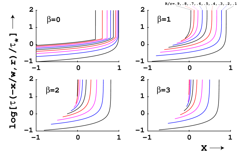
Figure 1: Log of the scaled optical depth $\tau[-x/w(r),r]/\tau_{\mathchar 8707\relax}$ vs. the scaled wavelength $x$, at selected radii $r$ in models with $\beta=$ 0, 1, 2, and 3. These contours effectively show the degree of wind attenuation as a function of wavelength for a source at a given radius.

2.2 Line-Emission Integration

Let us next consider the line emissivity, which we take here to be of the form

$$\eta_{\lambda}(r,\mu)=C\rho^{2}(r)f(r)\,\delta\left[\lambda-\lambda_{o}(1-\mu v(r)/c)\right],$$ (6)

where $C$ is an emission normalization constant, $\lambda_{o}$ is the rest wavelength for the line-emission, and $f(r)$ represents a volume filling-factor for X-ray emission. Note that the radial dependence of this filling factor may reflect variations in the temperature distribution of the plasma, as well as variations in the total emission measure.

The form (6) simply assumes the emission is an arbitrarily sharp function centered on the local, Doppler-shifted, comoving-frame wavelength $\lambda_{o}(1-\mu v(r)/c)$, and so ignores all broadening (e.g., natural, Stark, thermal, turbulent). For Doppler shifts associated with either thermal or small-scale “micro-turbulent” motions, the delta-function should be replaced with a finite-width emission profile. But generally, such microscopic motions can be expected to be no greater than the gas sound speed, which for X-ray emitting plasma of temperature $T_{x}\sim 10^{7}$ K is of order a few times 100 km ${\rm s}^{-1}$. As such, the associated broadening should be relatively small compared to that expected from the directed motion of the wind outflow, which has a much larger characteristic speed $v_{\infty}>1000$ km ${\rm s}^{-1}$. Moreover, as discussed in §3.2, for larger-scale, “macro-turbulent” motions, the effects can be taken into account a postori by incorporating them with the general smearing of the observed line profiles expected from the limited spectral resolution of the X-ray detector.

For convenience, let us define a scaled wavelength measured from line center in units of the wind terminal speed $v_{\infty}$, i.e. $x\equiv(\lambda/\lambda_{o}-1)c/v_{\infty}$. In terms of this scaled wavelength, the integrals (1) for the luminosity spectrum then become

$$L_{x}=8\pi^{2}C\int_{-1}^{1}\,d\mu\,\int_{{R_{\mathchar 8707\relax}}}^{\infty}\,dr\,r^{2}\,f(r)\rho^{2}(r){e}^{-\tau[\mu,r]}\,\delta(x+\mu w(r))\,,$$ (7)

where we have used the convention $L_{x}dx=L_{\lambda}d\lambda$. Integrating the Dirac $\delta$-function over direction cosine $\mu$, we then find that the wavelength-dependent X-ray luminosity can be evaluated from the single radial integral,

$$L_{x}={C\dot{M}^{2}\over 2v_{\infty}^{2}}\int_{{R_{\mathchar 8707\relax}}}^{\infty}\,dr\,H\left[w(r)-|x|\right]\,{f(r)\over r^{2}w^{3}(r)}\,{e}^{-\tau\left[-x/w(r),r\right]}\,,$$ (8)

where $H$ is the Heaviside (a.k.a. unit-step) function, with $H(s)=1$ if $s\geq 0$, and zero otherwise.

Figure 1 plots the optical depth $\tau[-x/w(r),r]$ versus scaled wavelength $x$ at selected radii $r$ in models with various $\beta$. For each radius, there is a critical, positive wavelength $x$ where the optical depth increases steeply, representing the strong attenuation of the red-wing emission by the dense inner wind and stellar core. Such core occultation makes the integrand in eqn. (9) effectively zero for all $u$ where $(1-u)^{\beta}\sqrt{1-u^{2}}<x$. For blue-wing wavelengths $x<0$, the termination of the curves indicates the maximum blue-shift allowed by the velocity at the relevant radius.

Ignace (2001) has recently derived completely analytic results for the X-ray profiles assuming a power-law emission factor $f(r)\sim r^{-q}$ and constant outflow velocity, $\beta=0$ (implying $w(r)=1$). As noted above, for the somewhat more general case of nonzero, but integer values of $\beta$, the optical depth integral (4) can still be done analytically; but in general the radial integral (8) must be evaluated by numerical quadrature. For this numerical integration, it is convenient (following Ignace (2001)) to define an inverse radius coordinate $u\equiv{{R_{\mathchar 8707\relax}}}/r$, yielding

$$L_{x}={C\dot{M}^{2}\over 2v_{\infty}^{2}{{R_{\mathchar 8707\relax}}}}\int_{0}^{u_{x}}\,du{f(R_{\mathchar 8707\relax}/u)\over(1-u)^{3\beta}}\,{e}^{-\tau\left[-x/(1-u)^{\beta},{{R_{\mathchar 8707\relax}}}/u\right]}\,,$$ (9)

where $u_{x}\equiv 1-|x|^{1/\beta}$.

3 Results for Normalized Line Profiles from Power Law X-ray Emission

For any chosen model for the spatial variation of emission $f(r)$, eqn. (9) can be readily evaluated through a single numerical integration. As a specific illustration, we now present results for the example case of an emission factor with the power-law form $f(r)=f_{\mathchar 8707\relax}u^{q}$ for radii $r\equiv{{R_{\mathchar 8707\relax}}}/u>R_{o}\equiv{{R_{\mathchar 8707\relax}}}/u_{o}$, and zero otherwise. This cutoff implies a slight redefinition to the upper integral bound in eqn.(9),

$$u_{x}\equiv\min\left[u_{o},1-|x|^{1/\beta}\right]\,.$$ (10)

To focus on the general form of X-ray line emission, let us define a normalized emission profile,

$$l_{x}\equiv{L_{x}\over\max_{x}[L_{x}]},$$ (11)

which simply sets the profile maximum to have a value of unity. This effectively removes the dependence on the several free parameters (e.g. $f_{\mathchar 8707\relax}$, $\dot{M}$, $v_{\infty}$, etc.) that affect the overall emission normalization. The form of the resulting X-ray line-profile $l_{x}$ versus scaled wavelength $x$ thus depends on four free parameters, viz. $\beta$, $\tau_{\mathchar 8707\relax}$, $q$, and $R_{o}/{{R_{\mathchar 8707\relax}}}$. The effects of wind attenuation and other model parameters on the overall X-ray emission level have been addressed in a broad-band context by Owocki & Cohen (1999), but in focussing here on line profile shapes, we defer to future work any analysis of the overall emission line strength.

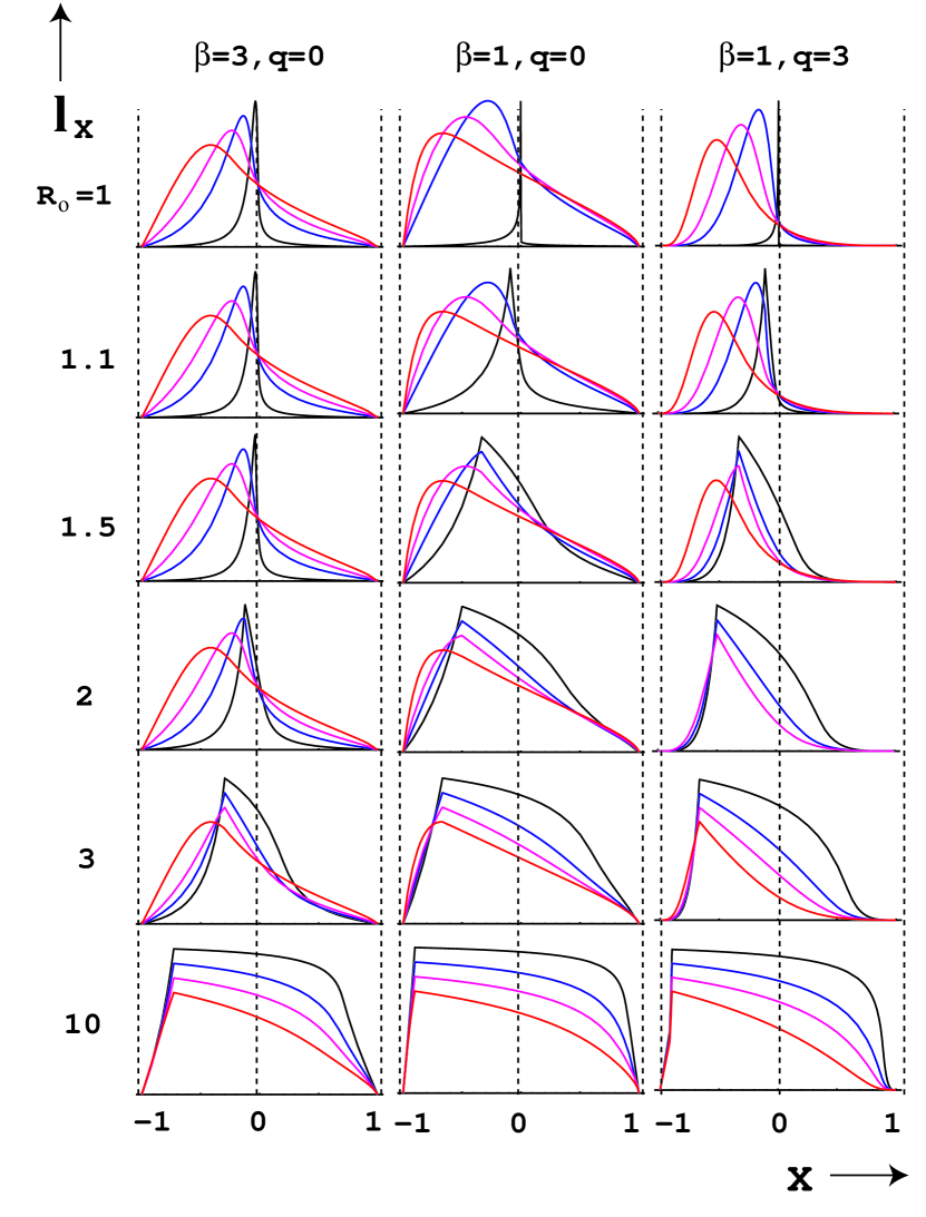
Figure 2: Scaled emission profile $l_{x}$ vs. the scaled wavelength $x$, plotted for various parameter combinations. In each box, profiles for optical depths $\tau_{\mathchar 8707\relax}=$ 1, 3, 5, and 10 are overplotted, with the various curves distinguished by having their peak values scaled respectively by factors of 1, 0.9, 0.8, and 0.7. The six rows represent, from the top to bottom, cases with initial emission radii of $R_{o}/{{R_{\mathchar 8707\relax}}}=$ 1, 1.1, 1.5, 2, 3, and 10. The central of the three columns represents a ‘standard’ case with $\beta=1$ and $q=0$, while the columns to each side illustrate cases which differ from this standard by setting $\beta=3$ (left) or $q=3$ (right).

3.1 Synthetic Emission Line Profiles for Various Model Parameters

Figure 2 presents synthetic emission profiles for various combinations of these parameters, all plotted vs. the scaled wavelength $x$ over the range $-1<x<1$. For comparison, figure 3 shows the flat-topped profiles for corresponding cases with optically thin emission, $\tau_{\mathchar 8707\relax}=0.01$. Some notable general properties and trends are as follows:

• The profiles seem most sensitive to $\tau_{\mathchar 8707\relax}$ and $R_{o}$, with $\beta$ and $q$ having a comparatively modest influence.

• The emission peaks are always blueward of line center (i.e., at $x<0$), with increasing blueshift for increasing $\tau_{\mathchar 8707\relax}$ and/or increasing $R_{o}$.

• The overall line-width likewise increases with increasing $\tau_{\mathchar 8707\relax}$ and/or $R_{o}$. The narrowest lines occur when both $\tau_{\mathchar 8707\relax}$ and $R_{o}$ are near unity. Large $\tau_{\mathchar 8707\relax}$ with low $R_{o}$ tend to give blue-shifted “peaked” forms, while large $R_{o}$ tend to be blue-tilted “flat-top” forms.

• The blue-to-red slope near line center is always negative. For low $\tau_{\mathchar 8707\relax}$ it varies from very steep for low $R_{o}$ to nearly flat for large $R_{o}$. For large $\tau_{\mathchar 8707\relax}$ it has a more intermediate steepness for all $R_{o}$.

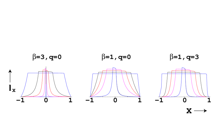
Figure 3: Flat-topped emission profiles for the optically thin case $\tau_{\mathchar 8707\relax}=0.01$. The left, center, and right box correspond to the same wind parameters as in figure 2, but the five overplots in each box now represent cases with initial emission radii at $R_{o}/{{R_{\mathchar 8707\relax}}}=$ 1.1, 1.5, 2, 3, and 10, with the various curves now distinguished by having their peak values scaled respectively by factors of 1, 0.95, 0.9, 0.85, and 0.8.

3.2 Broadened Profiles for Coronal vs. Wind-Shock Scenarios

For this simple parameterized model, the profiles presented above represent the expected intrinsic line emission, with the only broadening associated with the directed, large-scale wind outflow. In practice, observed line profiles can be further broadened, both by the limited spectral resolution of the detector, as well as by Doppler shifting from additional, random motions of the emitting gas. As already noted in §2.2, for small-scale thermal or “micro-turbulent” motions, the associated broadening can be expected to be no larger than the gas sound speed, which for $T_{x}\sim 10^{7}$ K plasma is order a few 100 km ${\rm s}^{-1}$. Since this is much less than the $v_{\infty}>1000$ km ${\rm s}^{-1}$ characteristic of the directed wind outflow, it should have comparitatively minor effect on line-profiles arising from the outer wind. For the inner wind or a more static “coronal” models, larger-scale turbulent broadening, which might in principle have a larger characeristic speed, can still be accounted for a postori, together with instrumental broadening arising from the limited spectral resolution of the detectors used in the XMM and Chandra satellites. For simplicity, we assume here that both macro-turbulent and instrumental broadening can be characterized by convolving a simple Gaussian kernel function over the intrinsic line-profile. As such, a single parameterized width $\sigma$, defined here in units of the wind terminal speed $v_{\infty}$, represents the combined effects of both any macroturbulent motion and intrumental broadening, with $\sigma\equiv\sqrt{\sigma_{turb}^{2}+\sigma_{instr}^{2}}$.

Let us now consider examples of such broadened line-profiles. To keep the parameter range tractable, we identify specific parameter subsets to represent general conditions in the two distinct scenarios that have often been invoked in modeling hot-star X-ray emission, namely the “coronal” (e.g., Waldron, 1984) vs. “wind-shock” scenarios (e.g., Feldmeier, Puls, & Pauldrach, 1997; Owocki & Cohen, 1999). The coronal scenario envisions X-ray emission as coming mostly from a relatively narrow, nearly static layer near the stellar surface; we represent this here with the parameter values $q=5$, $\beta=3$, and $R_{o}={{R_{\mathchar 8707\relax}}}$. The wind-shock scenario generally envisions X-ray production arising from instability-generated shocks that form in the acceleration region $r=1-3{{R_{\mathchar 8707\relax}}}$ of the star’s line-driven wind, with eventual slow decay of the shocks in the outer wind; we represent this here with the parameter values $R_{o}=1.5{{R_{\mathchar 8707\relax}}}$, $\beta=1$, and $q=0.5$. For both scenarios we again consider the effect of various optical depth parameters, $\tau_{\mathchar 8707\relax}$.

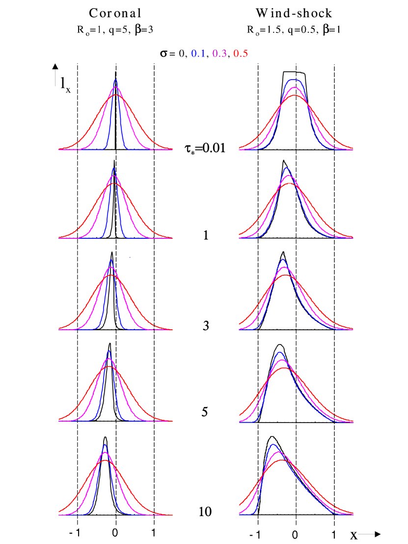
Figure 4: As in figure 2, scaled emission profile $l_{x}$ vs. the scaled wavelength $x$, but now comparing results for a coronal (left) vs. wind-shock (right) scenario. The four overplots now represent profiles with broadening parameters set to $\sigma=$ 0, 0.1, 0.3 and 0.5, again with the overall emission scaled respectively by factor of 1, 0.9, 0.8, and 0.7. The five rows now represent (from the top) cases with optical depth parameters set respectively to $\tau_{\mathchar 8707\relax}=$ 0.01, 1, 3, 5, and 10.

Figure 4 compares results for the coronal (left) vs. wind-shock (right) scenario. In characterizing results, we shall refer to profiles with small vs. large $\sigma$ as representing good/high vs. coarse/low resolution. Here some notable general properties and trends include:

• At the best resolution ($\sigma=0.1$), the coronal models are, as expected, notably narrower than the wind models.

• The wind-shock models are generally more blue-shifted than the coronal models.

• At the coarsest resolution, ($\sigma=0.5$), all profiles have similar width, but still generally differ in overall blue-shift.

• For the optically thin case, the emission is nearly symmetric about line center. For other cases, the emission peaks become more blue-shifted with increasing optical depth $\tau_{\mathchar 8707\relax}$. (The coronal models with larger $\tau_{\mathchar 8707\relax}$ may not be relevant, however, since wind absorption would greatly reduce the overall strength of any observable emission.)

The typical spectral resolution for Chandra is around $\lambda/\Delta\lambda\sim 1000-1500$. For characteristic wind terminal speed of $v_{\infty}\sim 2000-3000$, this implies a typical broadening parameter of $\sigma\sim 0.1$. For XMM, the spectral broadening is comparable, though slightly larger. Clearly, at such high resolutions, it should be possible to place strong constraints on the site of X-ray emission and the degree of wind attenuation, as well as on the characteristic speeds of directed vs. turbulent motions of the emitting plasma.

4 Discussion

The parameterized emission models here provide a good basis for interpreting X-ray line-profile observations made possible by the new generation of orbiting X-ray telescopes. While detailed, quantitative analyses must await the general availability of specific datasets, it is already clear from the few hot-star X-ray spectra published thus far that there are some noteworthy challenges for modeling the associated X-ray emission.

For example, temperature-sensitive line-ratio diagnostics provide constraints on the magnitude of shocks in dynamical models. Generally instability generated wind-shock models tend to be dominated by moderate shock-strengths $\Delta v\sim 100-400$ km ${\rm s}^{-1}$ that can only heat material up to a maximum of $\sim 10^{7}$ K (Feldmeier et al., 1997). In those stars with much higher inferred temperatures, for example $\theta^{1}$ Ori C with $T>5\times 10^{7}$ K (Schulz et al., 2001), there is a need to produce stronger shocks. One possibilty is for wind outflow to be channeled by magnetic loops (Babel & Montmerle, 1997). In this case, wind material accelerated up opposite footpoints of a closed loop can be forced to collide near the loop top, in principle yielding shocks with velocity jumps of order $\Delta v\sim 1000$ km ${\rm s}^{-1}$, a substantial fraction of the wind terminal speed.

Another key diagnostic stems from the forbidden-to-intercombination (f/i) ratios of helium-like emission lines, which can provide a strong constraint on the location of the X-ray emission. In the case of the solar corona, such ratios are nominally interpreted as density diagnostics (Gabriel & Jordan, 1969). But because the strong UV radiation of hot-stars can generally dominate over electron collisions in the destruction of forbidden line upper levels, in such stars the f/i provides instead a constraint on the strength of the UV intensity (Blumenthal, Drake, & Tucker, 1972; Mewe & Schrijver, 1978). With appropriate atmospheric modeling of the relevant part of UV continuum, any inferred dilution of the radiation thus provides a diagnostic of the proximity of the X-ray emission to the stellar surface. For XMM observations of $\zeta$ Pup (Kahn et al., 2001), initial interpretations suggest formation well away from the stellar surface ($r>2{{R_{\mathchar 8707\relax}}}$), consistent with a wind-shock origin, with moreover a general trend toward larger radii for lower-energy lines, as would be expected from the larger optical depths and thus larger unit-optical-depth radii for such lines. For Chandra observations of $\zeta$ Ori Waldron & Cassinelli (2001), the inferred formation radii are also generally away from the star ($r\approx 2-10{{R_{\mathchar 8707\relax}}}$), but with one stage (Si XIII) suggesting a formation very close to the surface ($r<1.1{{R_{\mathchar 8707\relax}}}$). However, in this latter case, the relevant UV flux for destruction of the forbidden upper levels lies at energies above the Lyman-edge, and so any error in atmospheric modeling of the Lyman jump could still alter this inferred formation radius. Chandra observations of $\zeta$ Pup (Cassinelli et al., 2001) show similar results, with most inferred formation radii in the range $r\approx 1.5-10{{R_{\mathchar 8707\relax}}}$, with trends again consistent with inferred unit-optical-depth radii, but again with one stage (in this case S XV) implying formation quite close to the surface ($r<1.25{{R_{\mathchar 8707\relax}}}$). Of course, such fir constraints on source location must eventually be considered in conjunction with additional constraints, such as those provided by analysis of line profiles.

Indeed, in the context of this paper, the most notable new diagnostic provided by recent X-ray observations lies in the form of the line profiles. For some initial results, these have some quite puzzling characteristics. For example, in the XMM spectrum of $\zeta$ Pup (Kahn et al., 2001), the lines all exhibit a similar, significant broadening, but with half-widths $\sim 1000-1500$ km s^-1 that are still somewhat lower than the inferred wind terminal speed $v_{\infty}\mathrel{\hbox to0.0pt{\lower 3.0pt\hbox{$\mathchar 536\relax$}\hss}\raise 2.0pt\hbox{$\mathchar 318\relax$}}2000$ km s^-1. The typical profiles have a rounded, Gaussian form that is quite distinct from, e.g., the flat-topped profiles expected for optically thin emission from a nearly constant velocity expansion. Moreover, the profiles show only modest asymmetry, with the peak intensity only slightly blue-shifted, by $\sim 0-400$ km s^-1 relative to line-center, and the red-wing only slightly flatter and more extended than the blue-wing. Recent somewhat higher spectral resolution observations by Chandra do show the greater shift and asymmetry expected from optically thick wind emission for $\zeta$ Pup (Cassinelli et al., 2001). But in Chandra observations of the O9.7 Ib star $\zeta$ Ori, the profiles are again very broad (half-widths of $\sim$ 1000 km ${\rm s}^{-1}$), but nearly symmetric (Waldron & Cassinelli, 2001).

Such profiles with substantial broadening, but little asymmetry and blueshift are difficult to reconcile with a simple wind-outflow model that includes attenuation by the wind and stellar core, both of which should preferentially attenuate X-rays from the back-side hemisphere, and thus in a wind or a corona with some outflow, preferentially reduce the red-side emission. In fact, from detailed modeling constrained by ROSAT  observations, Hillier et al. (1993) have argued that that the wind of $\zeta$ Pup should be optically thick to 1 keV X-rays at 10 $R_{\mathchar 8707\relax}$, with the radius of optical depth unity being even greater for softer X-rays (20 $R_{\mathchar 8707\relax}$ at 0.6 keV; and still 2 $R_{\mathchar 8707\relax}$ at 2 keV).

Even for a base corona with some overall outflow velocity and no overlying wind attenuation, occultation by the stellar core should still produce line profiles that are skewed toward the blue. A coronal model with little or no net outflow could explain the observed profile symmetry, but matching the observed line-widths would then require the coronal material to have extremely large “turbulent” motions. For example, line widths in the Chandra observations of $\zeta$ Ori (Waldron & Cassinelli, 2001) require velocity dispersions of order 1000 km ${\rm s}^{-1}$, and some of the lines observed by Chandra in $\theta^{1}$ Ori C (Schulz et al., 2001) are even broader than this, yet apparently still nearly symmetric. If the lack of red-wing attenuation is interpreted to mean that red-shifted emission does not arise from wind outflow from the backside hemisphere, then this suggest that material in front of the star must be flowing downward at velocities of 1000 km ${\rm s}^{-1}$. Since this is greater than the surface escape speed, it cannot be the result of gravitational infall, but instead would imply that some mechanism, e.g., perhaps magnetic reconnection (Waldron & Cassinelli, 2001), must actively accelerate roughly equally strong upflow and downflow with speeds of 1000 km ${\rm s}^{-1}$! Moreover, such random motions should inevitably lead to high-speed gas collisions and their associated shock heating. For shocks with velocity jumps of order 1000 km ${\rm s}^{-1}$ the associated post-shock temperature should be of order $10^{8}$ K, implying generally harder X-rays and higher ionization stages than are typically observed. In this context, these broad but symmetric profiles would indeed seem to represent a strong challenge for theoretical models.

On the other hand, our synthesized line profiles from wind models do seem capable of producing relatively broad, yet symmetric and unshifted profiles, but only in the nearly complete absence of wind attenuation, and with emission originating far from the occultation of the stellar core. To test the viabilty of this alternative, observed line-profiles should be interpreted in conjunction with other diagnostics, like the f/i ratio, that can constrain the radii of X-ray emission, and with an accurate account of wind absorption, as computed through opacity calculations for the observationally inferred wind mass loss rate.

Any wind shock model with significant wind attenuation is expected to be strongly blueshifted and quite asymmetric (see figure 4). Of all the line profiles discussed in the first group of XMM and Chandra papers, the observations of $\zeta$ Pup provide the best evidence for the blue-shifts and asymmetry expected for optically thick wind emission (Kahn et al., 2001; Cassinelli et al., 2001). For example, figure 3 of Cassinelli et al. (2001) shows 5 out of 6 lines with blueward shifts and asymmetry similar to profiles calculated here for wind-shock models with substantial optical depth, e.g. $\tau_{\mathchar 8707\relax}\sim 5$. At least for this canonical O-type star, these profiles seems to provide strong evidence of a wind origin for most of the observed X-rays.

In summary, systematic fitting of the line-profiles will be necessary to place more quantitative constraints on the spatial distribution of hot plasma and the degree of wind attenuation in the observed O stars; but some initial qualitative inferences are already possible. For some cases, the implied minimal wind attenuation combined with some significant bulk motion are puzzling, both in the context of coronal X-ray emission and in the context of the strong radiation-driven winds that are known to exist on these stars from UV, optical, IR, and radio observations. One possible solution to the wind attenuation problem might be found in clumping. A “porous” wind might allow many of the X-rays to stream through unattenuated, yet also lead to significant UV absorption if the interclump wind medium still has sufficient column density to produce optically thick UV lines. (The UV line transition probabilities are significantly larger than the bound-free X-ray cross sections.) An alternative is that the mass-loss rates of O stars may have been overestimated. It does not seem likely, however, that the winds are dense and smooth but transparent to X-rays, as that would require levels of ionization in the wind that would not allow for efficient radiation-driving. And, if the winds are indeed optically thin, then to discriminate between coronal and wind models will require a careful analysis of the shifts and asymmetries observed in the X-ray line profiles.

Finally, although we developed our analysis with hot stars in mind, it could be extended to other X-ray sources in which lines are emitted within a nearly symmetric expanding medium that may also have substantial continuum opacity. This could include nova winds, planetary nebulae, active galactic nuclei, and X-ray binaries.

References

- Baade & Lucy (1987) Baade, D., & Lucy, L. 1987, A&A, 178, 213
- Babel & Montmerle (1997) Babel, J. & Montmerle, T. 1997, ApJ, 485, L29
- Berghöfer & Schmitt (1994) Berghöfer, T. W., & Schmitt, J. H. M. M. 1994, Ap&SS, 221, 309
- Blumenthal, Drake, & Tucker (1972) Blumenthal, G. R., Drake, G. W. F., & Tucker, W. H. 1972, ApJ, 172, 205
- Cassinelli et al. (1995) Cassinelli, J. P., Cohen, D. H., Macfarlane, J. J., Drew, J. E., Lynas-Gray, A. E., Hoare, M. G., Vallerga, J. V., Welsh, B. Y., Vedder, P. W., Hubeny, I., & Lanz, T. 1995, ApJ, 438, 932
- Cassinelli et al. (2001) Cassinelli, J. P., Miller, N. A., Waldron, W. L., MacFarlane, J. J., & Cohen, D. H. 2001, ApJ, in press
- Cassinelli & Olson (1979) Cassinelli, J. P., & Olson, G. L. 1979, ApJ, 229, 304
- Cassinelli, Olson, & Stalio (1978) Cassinelli, J. P., Olson, G. L., & Stalio, R. 1978, ApJ, 220
- Cassinelli & Swank (1983) Cassinelli, J. P., & Swank, J. H. 1983, ApJ, 271, 681
- Chlebowski, Harnden, & Sciortino (1989) Chlebowski, T., Harnden, F. R., Jr., & Sciortino, S. 1989, ApJ, 341, 427
- Cohen et al. (1996) Cohen, D. H., Cooper, R. G., MacFarlane, J. J., Owocki, S. P., Cassinelli, J. P., & Wang, P. 1996, ApJ, 460, 506
- Cohen, Cassinelli, & MacFarlane (1997) Cohen, D. H., Cassinelli, J. P., & MacFarlane, J. J. 1997, ApJ, 487, 867
- Feldmeier et al. (1997) Feldmeier, A., Kudritzki, R.-P., Palsa, R., Pauldrach, A. W. A., & Puls, J. 1997, A&A, 320, 899
- Feldmeier, Puls, & Pauldrach (1997) Feldmeier, A., Puls, J., & Pauldrach, A. W. A. 1997, A&A, 322, 878
- Gabriel & Jordan (1969) Gabriel, A. H., & Jordan, C. 1969, MNRAS, 145, 241
- Hillier et al. (1993) Hillier, D. J., Kudritzki, R. P., Pauldrach, A. W., Baade, D., Cassinelli, J. P., Puls, J., & Schmitt, J. H. M. M. 1993, A&A, 276, 117
- Ignace (2001) Ignace, R. 2001, ApJ, in press
- Kahn et al. (2001) Kahn, S. M., Leutenegger, M. A., Cotam, J., Rauw, G., Vreux, J.-M., den Boggende, A. J. F., Mewe, R., & Güdel, M. 2001, A&A, in press
- Long & White (1980) Long, K. S., & White, R. L. 1980, ApJ, 239, L65
- Lucy (1982) Lucy, L. 1982, ApJ, 255, 286
- Lucy & White (1980) Lucy, L. B., & White, R. L. 1980, ApJ, 241, 300
- MacFarlane et al. (1991) Macfarlane, J. J., Cassinelli, J. P., Welsh, B. Y., Vedder, P. W., Vallerga, J. V., & Waldron, W. L. 1991, ApJ, 380, 564
- MacFarlane et al. (1993) MacFarlane, J. J., Waldron, W. L., Corcoran, M. F., Wolff, M. J., Wang, P., & Cassinelli, J. P. 1993, ApJ, 419, 813
- Mewe & Schrijver (1978) Mewe R., & Schrijver, J. 1978, A&A, 65, 99
- Nordsieck, Cassinelli, & Anderson (1981) Nordsieck, K. H., Cassinelli, J. P., & Anderson, C. M. 1981, ApJ, 248, 678
- Owocki, Castor, & Rybicki (1988) Owocki, S. P., Castor, J. I., & Rybicki, G. B. 1988, ApJ, 335, 914
- Owocki & Cohen (1999) Owocki, S. P., & Cohen, D. H. 1999, ApJ, 520, 833
- Pallavicini et al. (1981) Pallavicini, R., Golub, L., Rosner, R., Vaiana, G. S., Ayres, T., & Linsky, J. L. 1981, ApJ, 248, 279
- Schulz et al. (2001) Schulz, N. S., Canizares, C. R., Huenemoerder, D., & Lee, J. C. 2001, ApJ, in press
- Snow & Morton (1976) Snow, T. P., Jr., & Morton, D. C. 1976, ApJS, 32, 429
- Waldron (1984) Waldron, W. L. 1984, ApJ, 282, 256
- Waldron & Cassinelli (2001) Waldron, W. L., & Cassinelli, J. P. 2001, ApJ, in press