Methods of Determination of the
Energy and Mass of Primary Cosmic Ray Particles
at Extensive Air Shower Energies

Abstract

Measurements of cosmic ray particles at energies above $E\mathrel{\mathchoice{\vbox{\offinterlineskip\halign{\hfil$\displaystyle#$\hfil\cr>\cr\sim\cr}}}{\vbox{\offinterlineskip\halign{\hfil$\textstyle#$\hfil\cr>\cr\sim\cr}}}{\vbox{\offinterlineskip\halign{\hfil$\scriptstyle#$\hfil\cr>\cr\sim\cr}}}{\vbox{\offinterlineskip\halign{\hfil$\scriptscriptstyle#$\hfil\cr>\cr\sim\cr}}}}5\cdot 10^{14}$ eV are performed by large area ground based air shower experiments. Only they provide the collection power required for obtaining sufficient statistics at the low flux levels involved. In this review we briefly outline the physics and astrophysics interests of such measurements and discuss in more detail various experimental techniques applied for reconstructing the energy and mass of the primary particles. These include surface arrays of particle detectors as well as observations of Cherenkov- and of fluorescence light. A large variety of air shower observables is then reconstructed from such data and used to infer the properties of the primary particles via comparisons to air shower simulations. Advantages, limitations, and systematic uncertainties of different approaches will be critically discussed.

1 Introduction

The cosmic ray (cr) energy spectrum extends from about 1 GeV to above $10^{20}$ eV. Over this wide range of energies the intensity drops by more than 30 orders of magnitude. Despite the enormous dynamic range covered, the spectrum appears rather structureless and can be well approximated by broken power-laws $dN/dE\propto E^{-\gamma}$. Up to energies of some $10^{14}$ eV the flux of particles is sufficiently high allowing measurements of their elemental distributions by high flying balloon or satellite experiments. Such studies have provided important implications for the origin and transport properties of cr’s in the interstellar medium. Two prominent examples are ratios of secondary to primary elements, such as the B/C-ratio, which are used to extract the average amount of matter cr-particles have traversed from their sources to the solar system, or are radioactive isotopes, e.g. ¹⁰Be or ²⁶Al, which carry information about the average ‘age’ of cosmic rays. With many new complex experiments taking data or starting up in the near future and with a possibly new generation of balloons, this is a vital field of research and has been subject to separate talks presented at this Symposium.

Above a few times $10^{15}$ eV the flux drops to only one particle per m² per year. This excludes any type of ‘direct observation’ even in the near future, at least if high statistics is required. Ironically, one of the most prominent features of the cr energy spectrum is the steepening of the slope from $\gamma\cong 2.7$ to $\gamma\cong 3.1$ at an energy just above some $10^{15}$ eV. This is known as the ‘knee’ of the spectrum. It was first deduced from observations of the shower size spectrum made by Kulikov and Khristianson et alin 1956 [1] but it still remains unclear as to what is the cause of this spectral steepening. At an energy above $10^{18}$ eV the spectrum flattens again at what is called the ‘ankle’. Data currently exist, though with very poor statistics, up to $3\cdot 10^{20}$ eV and there seems to be no end to the energy spectrum [2, 3].

The origin and acceleration mechanism of these, so called, ultra- and extremely high energy cosmic rays have been subject to debate for several decades. Mainly for reasons of the required power the dominant acceleration sites are generally believed to be shocks associated with supernova remnants. Naturally, this leads to a power law spectrum as is observed experimentally. Detailed examination suggests that this process is limited to $E/Z\mathrel{\mathchoice{\vbox{\offinterlineskip\halign{\hfil$\displaystyle#$\hfil\cr<\cr\sim\cr}}}{\vbox{\offinterlineskip\halign{\hfil$\textstyle#$\hfil\cr<\cr\sim\cr}}}{\vbox{\offinterlineskip\halign{\hfil$\scriptstyle#$\hfil\cr<\cr\sim\cr}}}{\vbox{\offinterlineskip\halign{\hfil$\scriptscriptstyle#$\hfil\cr<\cr\sim\cr}}}}10^{15}$ eV. Curiously, this coincides well with the knee at $E_{\rm knee}\cong 4\cdot 10^{15}$ eV, indicating that the feature may be related to the upper limit of acceleration. The underlying picture of particle acceleration in magnetic field irregularities in the vicinity of strong shocks suggests the maximum energies of different elements to scale with their rigidity $R=pc/Ze$. This naturally would lead to an overabundance of heavy elements above the knee, a prediction to be proven by experiments. A change in the cr propagation with decreasing galactic containment at higher energies has also been considered. This rising leakage results in a steepening of the cr energy spectrum and again would lead to a similar scaling with the rigidity of particles but would in addition predict anisotropies in the arrival direction of cr’s with respect to the galactic plane. Besides such kind of ‘conventional’ source and propagation models [4, 5] several other hypotheses have been discussed in the recent literature. These include the astrophysically motivated single source model of Erlykin and Wolfendale [6] trying to explain possible structures around the knee, as well as several particle physics motivated scenarios which try to explain the knee due to different kinds of cr-interactions. For example, photodisintegration at the source [7], interactions with gravitationally bound massive neutrinos [8], or sudden changes in the character of high-energy hadronic interactions during the development of extensive air shower (eas) [9] have been considered.

To constrain the SN acceleration model from the other proposed mechanisms precise measurements of the primary energy spectrum and particularly of the mass composition as a function of energy are needed. Significant progress has been made on these problems in recent years, but the situation is far from being clear.

The other target of great interest is the energy range around the Greisen-Zatsepin-Kuzmin (gzk) cut-off at $E\simeq 5\cdot 10^{19}$ eV. Explanation of these particles requires the existence of extreme powerful sources within a distance of approximately 100 Mpc. Hot spots of radio galaxy lobes – if close enough – or topological defects from early epochs of the universe would be potential candidates. This topic has been addressed at this Symposium in some detail by Ostrowski, Zavrtanik, and others. Therefore, I will be very brief on experimental aspects relevant to measurements in this energy range.

2 Extensive Air Showers and Experimental Observables

An air shower is a cascade of particles generated by the interaction of a single high energy primary cosmic ray particle with the atmosphere. The secondary particles produced in each collision - in case of a primary hadron mostly charged and neutral pions - may either decay or interact with another nucleus, thereby multiplying the particles within an eas. After reaching a maximum ($X_{max}$) in the number of secondary photons, electrons, muons, and hadrons, the shower attenuates as more and more particles fall below the threshold for further particle production. A disk of relativistic particles extended over an area with a diameter of some tens of meters at $10^{14}$ eV to several kilometre at $10^{20}$ eV can then be observed at ground. This magnifying effect of the earth atmosphere allows to instrument only a very small portion of the eas area and to still reconstruct the major properties of the primary particles. It is a lucky coincidence that at the energy where direct detection of crs rays becomes impractical, the resulting air showers become big enough to be easily detectable at ground level.

Due to the nature of the involved hadronic and electromagnetic interactions and the different decay properties of particles, an eas has three components, electromagnetic, muonic, and hadronic. On average, a 1 PeV primary proton will produce about $10^{6}$ particles at sea-level, 80 % of which are photons, 18 % electrons, 1.7 % muons, and about 0.3 % hadrons. Neutrinos will also be produced by weak decays of particles, but they remain unseen by ordinary eas experiments. During their propagation through the atmosphere, relativistic charged particles will also produce Cherenkov light and, finally, excitations of the $2P$ and $1N$-band of N₂ and N${}_{2}^{+}$, respectively, will give rise to emission of fluorescence light.

Extracting the primary energy and mass from such measurements is not straightforward and a model must be adopted to relate the observed eas parameters to the properties of the primary particle. As shall be discussed below, the analysis is complicated by large fluctuations of eas observables and by the fact, that virtually all of the eas observables are sensitive to changes in the mass and energy of the primary particle so that a careful reconstruction of the energy spectrum requires knowledge of the chemical composition.

Ignoring these complications for a moment, some basic characteristics of eas, as observed in Fig. 1, can be deduced from very simple considerations. On average, the first interaction of the primary particle with a nucleus in the atmosphere - mostly nitrogen - will occur within its characteristic interaction length, $\lambda_{I}\propto 1/\sigma$. Due to the larger hadronic cross section of a Fe+N system as compared to p+N, the iron nucleus will - on average - interact higher in the atmosphere. Because of the strong absorption of the electromagnetic and hadronic shower components in the atmosphere, one expects

Figure 1: CORSIKA [10] simulations of the longitudinal shower development using the QGJSET [11] hadronic interaction model. The two thick lines represent averages of the individual p and Fe showers.

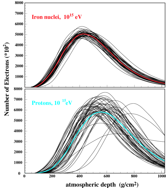
to detect fewer electrons and hadrons at ground in case of primary heavy nuclei. In a simplified picture, we furtheron may consider the primary iron nucleus as 56 nucleons each having 1/56^th of the primary energy. This has two important consequences: i) the energy of produced particles within a single collision will be lower by about the same number, so that more pions and kaons have a chance to decay into muons before reinteracting with another air nucleus, ii) the multiplicity of produced particles within a single high energy collision roughly scales with the logarithm of the energy, so that 56 nucleons each with 1/56^th of the energy, will produce a higher number of secondary particles, which again may decay into muons. As a result of the two effects one expects to observe more muons at ground in case of heavy primaries. Also, fluctuations in the number of particles will be smaller in case of heavy primary nuclei. Major experiments performing particle measurements at ground in the energy range of the knee include CASA-MIA [12], EAS-TOP [13], HEGRA [14], KASCADE [15, 16], and Tibet-AS$\gamma$ [17], only the latter two of which currently take data. Most of the data in the gzk energy range are based on the Akeno Giant-Air-Shower-Experiment (AGASA) [18]. Their primary observables are lateral particle density distributions at ground, $\rho_{e,\mu,h}(r)$, and their integrals $N_{e,\mu,h}=\int_{r_{1}}^{r_{2}}2\pi r\rho_{e,\mu,h}(r)dr$, yielding total (for extrapolations $r_{1}\to 0$ and $r_{2}\to\infty$) or truncated particle shower sizes. Truncated muon-sizes, $N_{\mu}^{\rm tr}$, have been introduced by the KASCADE collaboration in order to avoid systematic uncertainties resulting from extrapolations of $\rho_{\mu}(r)$ to large distances not covered by the experiment.

Table 1: Compilation of experimental eas observables and operating experiments. References are given in the text.

Measurement of	Observables	Energy Ranges	Operating Expts.
charged particles	shower size	$\mathrel{\mathchoice{\vbox{\offinterlineskip\halign{\hfil$\displaystyle#$\hfil\cr>\cr\sim\cr}}}{\vbox{\offinterlineskip\halign{\hfil$\textstyle#$\hfil\cr>\cr\sim\cr}}}{\vbox{\offinterlineskip\halign{\hfil$\scriptstyle#$\hfil\cr>\cr\sim\cr}}}{\vbox{\offinterlineskip\halign{\hfil$\scriptscriptstyle#$\hfil\cr>\cr\sim\cr}}}}5\cdot 10^{13}$ eV	GRAPES,
	lateral density distr.		KASCADE,
	arrival time distr.		Maket ANI, SPACE
muons	muon size	$\mathrel{\mathchoice{\vbox{\offinterlineskip\halign{\hfil$\displaystyle#$\hfil\cr>\cr\sim\cr}}}{\vbox{\offinterlineskip\halign{\hfil$\textstyle#$\hfil\cr>\cr\sim\cr}}}{\vbox{\offinterlineskip\halign{\hfil$\scriptstyle#$\hfil\cr>\cr\sim\cr}}}{\vbox{\offinterlineskip\halign{\hfil$\scriptscriptstyle#$\hfil\cr>\cr\sim\cr}}}}5\cdot 10^{13}$ eV	KASCADE,
	lateral muon distr.		AGASA ($>10^{18}$ eV)
	arrival time distr.
	$\mu$-production height	$\mathrel{\mathchoice{\vbox{\offinterlineskip\halign{\hfil$\displaystyle#$\hfil\cr>\cr\sim\cr}}}{\vbox{\offinterlineskip\halign{\hfil$\textstyle#$\hfil\cr>\cr\sim\cr}}}{\vbox{\offinterlineskip\halign{\hfil$\scriptstyle#$\hfil\cr>\cr\sim\cr}}}{\vbox{\offinterlineskip\halign{\hfil$\scriptscriptstyle#$\hfil\cr>\cr\sim\cr}}}}10^{15}$ eV
hadrons	hadron size	$5\cdot 10^{13}$ - $10^{17}$	KASCADE
	lateral hadron distr.	(practical limit
	energy distribution	by detector
	spatial correlations	area)
Cherenkov light	Cherenkov size	$5\cdot 10^{13}$ - $10^{17}$	BLANCA, HEGRA
	lateral Ch. distr.	(practical limit	DICE, TUNKA
	shower shape	by area of Ch.-cone)
Fluorescence light	total light yield	$\mathrel{\mathchoice{\vbox{\offinterlineskip\halign{\hfil$\displaystyle#$\hfil\cr>\cr\sim\cr}}}{\vbox{\offinterlineskip\halign{\hfil$\textstyle#$\hfil\cr>\cr\sim\cr}}}{\vbox{\offinterlineskip\halign{\hfil$\scriptstyle#$\hfil\cr>\cr\sim\cr}}}{\vbox{\offinterlineskip\halign{\hfil$\scriptscriptstyle#$\hfil\cr>\cr\sim\cr}}}}10^{17}$ eV	HIRes
	longitudinal profile	(limited by
	time profile	signal/noise)

Table 2: Compilation of eas observables and their sensitivity to primary energy and mass. (^(∗): energy estimates dependent also on primary mass)

Energy determination	Mass determination
$a\cdot\lg N_{\mu}+b\cdot\lg N_{e}$	$\lg N_{e}/\lg N_{\mu}$
	shape of electron lateral distribution; age-parameter
	mean muon production height
	muon arrival time distributions
	$\lg N_{h}/\lg N_{\mu}$, $\lg\sum E_{h}/\lg N_{\mu}$, spatial distr. of hadrons
	fluctuations of eas parameters, e.g. $\lg(N_{\mu})/\lg(\overline{N}_{\mu})$
$\rho_{Ch}(120)$ (∗)	non-imaging counters: inner Cherenkov slope
total Ch. light (∗)	Ch. telescopes: shape of shower image
	(the Ch. observables are often considered a measure of $X_{max}$)
total fluorescence light	position of shower maximum

Besides measuring particles at ground, experiments also aim at observing traces of the longitudinal shower development. A basic parameter here is the position of the shower maximum, $X_{max}$, which penetrates deeper into the atmosphere with increasing primary energy and decreasing primary mass. Experimentally, $X_{max}$ is often inferred from the lateral density distribution of Cherenkov photons, $\rho_{Ch}$. Experiments following this approach include CASA-BLANCA [19] and the HEGRA AIROBICC detectors [20]. Also, air Cherenkov telescopes have been employed for sampling the shower maximum (HEGRA [14], DICE [21]), and more recently, $X_{max}$ has been reconstructed from muon tracks at ground by means of triangulation (HEGRA [22] and KASCADE (talk presented by C. Büttner at this Symposium)). A very elegant approach is the detection of air fluorescence light at large distances from the shower axis giving true information about the longitudinal development of the eas. The major drawback is the low light yield limiting its application to energies $E\mathrel{\mathchoice{\vbox{\offinterlineskip\halign{\hfil$\displaystyle#$\hfil\cr>\cr\sim\cr}}}{\vbox{\offinterlineskip\halign{\hfil$\textstyle#$\hfil\cr>\cr\sim\cr}}}{\vbox{\offinterlineskip\halign{\hfil$\scriptstyle#$\hfil\cr>\cr\sim\cr}}}{\vbox{\offinterlineskip\halign{\hfil$\scriptscriptstyle#$\hfil\cr>\cr\sim\cr}}}}10^{17}$ eV. This technique pioneered by Fly’s Eye [23], is being employed by HIRes [24] and the Pierre Auger Observatory [25]. A summary of the different experimental observables is given in table 2. Deep underground muon detectors are omitted here because of limited space and because of their only indirect relation to eas observations.

3 Techniques of Data Analysis and Selected Results

3.1 Single parameter methods

Until recently, most experiments have performed single parameter analyses using only one of the eas observables discussed above. The composition has then been inferred by comparing the mean value of the experimental observable to either different trial composition models or to mean values of simulated proton and iron primaries and interpolations to a hypothetical ‘mean mass’. Obviously, a significant piece of information available from the full distribution of shower observables is ignored in such analyses. The problems here are manifold, most importantly: i) the extracted mean mass is ambiguous, i.e. the mean values of the experimental distribution can be described by a single ‘mean mass’ component, by a mix of pure protons and iron, or by any other combination. Clearly, a ‘composition’ in a strict sense is not obtained. ii) There is no clue of how well the simulations describe the experimental data. Only if the mean value of the experimental observable falls outside the window spanned by

Figure 2: The mean depth of shower maximum $X_{max}$ as a function of energy deduced from CASA-BLANCA [26]. The lines represent the values for pure proton and pure iron samples as predicted by different hadronic interaction models.

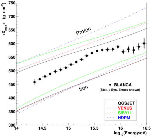
proton and iron simulations, doubts can be raised about the quality of the simulations (or apparatus). Furthermore, publications discussing single parameter results often do another simplification by comparing measured and simulated observables not at the level of the detector, but instead comparing quantities which are inferred from experimental data by means of eas simulations. A very prominent example of such kind of analyses are plots of $X_{max}$ as a function of energy as shown in Fig. 2. In this and many other cases, $X_{max}$ is based on measurements of the slope of the Cherenkov lateral distribution within about 120 m from the shower core. eas simulations using different primary particles are then performed to convert this experimental slope parameter to $X_{max}$. Finally, this biased and model dependent $X_{max}$-value is presented in such graphs and compared to $X_{max}$-values obtained directly from CORSIKA simulations. Clearly, comparing experimental and simulated slope parameters directly instead of introducing secondary quantities appears much more appropriate and avoids sources of systematic biases. Determination of $E_{prim}$ in experiments using open Cherenkov counters is mostly based on the Cherenkov light intensity observed at about 120 m from the shower core where influences of the unknown primary mass are minimal. However, a careful analysis of this procedure exhibits a residual mass dependence on the order of $\pm 10$ % in the knee energy range [27]. Also, uncertainties to the energy scale by at least the same amount are caused by hadronic interaction models [26] but, again, are not considered in plots of the type of Fig. 2. Finally, the figure also nicely demonstrates the aforementioned inabilities to judge the quality of the different hadronic interactions models or to infer a true composition. Despite this criticism, the qualitative feature of the data – a somewhat lighter ‘mean mass’ towards the knee and a heavier one above – appears common to all interaction models.

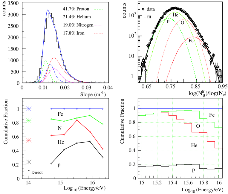
With increasing computer power, eas simulations have advanced in quality and quantity, i.e. both the complexity to which details of hadronic interactions and propagation effects in the atmosphere are taken into account has been improved as well as the number of simulated events available for comparison. Therefore, analyses of eas data could progress from comparing only mean values to full distributions of observables, the benefits of which have been discussed already. Two examples are presented in Fig. 3. The left hand side of the top panel presents the event-by-event distribution of the inner Cherenkov-slope (previously used as a measure for $X_{max}$, see above) in an energy range $8\cdot 10^{14}\leq E\leq 2\cdot 10^{15}$ eV [26] and the right hand side the distribution of $\log N_{\mu}^{\rm tr}/\log N_{e}$ obtained from KASCADE for zenith angles $18^{\circ}$ - $25^{\circ}$ and similar energies [28]. Both data sets are compared to CORSIKA simulations of different primary particles using the QGSJET model. Note, that the left hand tails of the distributions are well accounted for by proton simulations while the right hand tails are accounted for by iron simulations. The KASCADE distributions cover more than three orders of magnitude and thus provide some level of confidence in the results of the simulations. Both data sets also require at least 3 different primary masses to account for the full shape of the experimental distributions. However, it is also observed that the Cherenkov data alone do not provide sufficient discrimination power to distinguish the nitrogen from the iron distribution. The bottom panel shows the extracted mass fractions as a function of energy. Clearly, a heavier composition is observed at energies above the knee. Also, the relative abundance of iron is fairly similar in both data sets but the major difference is a reversed proton and Helium abundance resulting in a somewhat lighter composition from KASCADE data. To resolve this differences, several cross checks of the two data sets appear expedient, e.g. tests of the zenith angle dependence, still higher statistics in simulations to verify the tails of the distributions, etc. Such work is in progress now.

Figure 3: Event-by-event distributions of the inner Cherenkov slope (l.h.s.) [26] and of the muon/electron ratio (r.h.s.) [28]. The lower panel shows the cumulative fractions of different primary particles as a function of their energy.

3.2 Multi-component methods and non-parametric approaches

Multi-component detector installations can measure several eas parameters simultaneously on an event-by-event basis. Proper combinations can then be identified to provide an estimate of the primary energy and mass (see Table 1,2). The analysis of multivariate parameter distributions also needs to account for influences of fluctuations which may be different in different observables. Non-parametric Bayesian methods and neural network approaches are well suited for these purposes and they also specify the uncertainty of the results in a quantitative way [29]. Simpler approaches, like the knn-method have also been employed [30], but they suffer from various deficiencies like dependencies of the results on the density and thereby on the statistics of simulated data points.

First comprehensive non-parametric approaches with promising results have been presented at this Symposium by M. Roth et al. In these techniques, each event is represented by an observation vector $x=(N_{\mu}^{\rm tr}$, $N_{e}$, $N_{h}\ldots)^{T}$ of $n$ suitable eas observables. This vector serves as input to a procedure based on Bayesian or neural network decision rules by which the observed event is assigned to a given class of elemental groups, say p, O, and Fe. The first step in such an analysis is a calculation of likelihood (probability density) distributions $p(x|\omega_{i})$ by means of Monte Carlo simulations using different primary particles. Here, $p(x|\omega_{i})$ describes the probability to observe the multi-dimensional observation vector $x$ in an event belonging to a given class $\omega_{i}\in\{$p, O, Fe$\}$. The term ‘non-parametric’ indicates that the representations of the distributions (like probability density functions of Bayes classifiers or weights of neural networks) are no more specified by a-priori chosen functional forms, but are constructed through the analysis process by the given (simulated) data distributions themselves. Using the Bayes theorem one can then translate the likelihood $p(x|\omega_{i})$ for finding an event $x$ in a given class $\omega_{i}$ to the actually required distribution $p(\omega_{i}|x)$ representing the probability of class $\omega_{i}$ being associated to a measured event $x$. In this step, an assumption is made about an a priori knowledge of the relative abundance of each class, a subject being handled by Bayesian inference procedures. If there is no further knowledge, the prior probabilities should be assumed to be equal (Bayes’ Postulate).

Analysing an experimentally measured event, a statistical decision on the primary particle type/energy is then to be made. The applied Bayesian approach of the statistical inference provides the Bayes optimal way of combining prior and experimental knowledge and the Bayes theorem specifies how such modification should be made [31]. In simplest case, the Bayes optimal decision rule is to classify $x$ into class $\omega_{i}$, if $p(\omega_{i}|x)>p(\omega_{j}|x)$ for all classes $\omega_{j}\neq\omega_{i}$. In this way one is also able to specify the actual quality of the decision by classification and misclassification matrices of the results. Unfortunately, because of limited computer time, analyses making use of all these pieces of important information have not yet been performed for high statistics data. However, good agreement to faster neural network approaches was reported in Ref. [32].

It is important to realize that the composition extracted that way yields a somewhat heavier composition as compared to the results from Fig. 3. This effect may possibly be caused by different treatments of correlations among the fluctuating eas observables. Furthermore, detailed investigations also show that within a given interaction model, different sets of eas observables lead to different mass compositions [32]. Generally, inclusion of hadronic observables tends to shift the composition to a heavier one, a result already suggested by earlier studies of the KASCADE collaboration [33]. These inconsistencies appear to be caused by deficiencies of the employed hadronic interaction models. Both kinds of effects are subject to further studies and, at present, any quantitative result on chemical composition may be subject to further changes.

Results on chemical composition are often presented in terms of the mean logarithmic mass. However, this quantity has some severe drawbacks as any information about individual abundances is lost. Furthermore, in absence of an unique prescription on how to calculate the average from abundances of different mass groups, uncertainties in $\langle\ln A\rangle$ may be on the order of 0.2 and more. This has been source for some confusion in the past and can best be avoided by providing tables of reconstructed abundances of

Figure 4: Primary energy spectrum as obtained from different experiments [34]. (See text for references.)

mass groups (including correlated uncertainties).

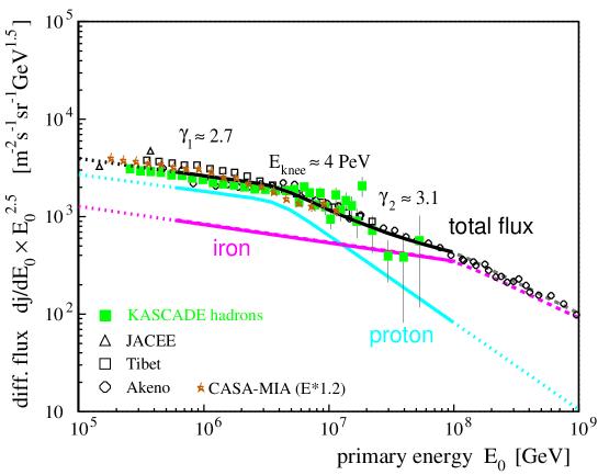
A compilation of the all-particle energy spectrum reconstructed from various experiments is presented in figure 4. The agreement appears reasonable and deviations are mostly explained by uncertainties in the energy scale by up to 25 %, e.g. CASA MIA data [35] were shifted upwards in energy by 20 % to yield a better agreement to the other data sets. This is likely to be explained by the interaction model SIBYLL 1.6 [36] employed by the authors of Ref. [35] but which has been proven to provide only a poor description of the experimental data [33]. The lines correspond to a simultaneous fit of the electron and muon size spectra of KASCADE, assuming the all-particle spectrum to be described by a sum of proton and iron primaries [34]. Interestingly, a knee is only reconstructed for the light component and no indication of a break is seen in the heavy component up to about $10^{17}$ eV. This important finding giving direct support to the picture of acceleration in magnetic fields (see above) will be target of future studies with improved experimental capabilities. For example, KASCADE and EAS-TOP have just started a common effort to install the EAS-TOP scintillators at the site of Forschungszentrum Karlsruhe providing a 12 times larger acceptance as compared to the original KASCADE experiment and still taking advantage of the multi-detector capabilities.

4 Summary and Outlook

Much progress has been made in reconstructing the parameters of primary cr-particles from eas observables. The advent of multiparameter measurements and realistic eas simulations now allow for much more detailed investigations taking account for eas fluctuations and detector effects. Different experiments agree fairly well on the all-particle energy spectrum but there is still some uncertainty in extracting the chemical composition. This may partly be explained by uncertainties of hadronic interaction models employed in eas simulations and there appears a demand for more tests of hadronic interaction models by means of accelerator and/or eas data. Other sources of systematic uncertainties appear to be caused by incomplete data analysis techniques and biases affecting mostly single parameter measurements. As discussions and presentations at this Symposium have shown, there is well founded hope to solve these imperfections thereby answering the question about the sources of crs and the origin of the knee already in the very near future.

Acknowledgement

I would like to express my gratitude to the organizing committee for their hospitality and inviting me to give this talk. During the preparation I greatly benefited from fruitful discussions with my colleagues from the KASCADE collaboration, with C. Pryke, J. Matthews, S. Swordy, and many others. I would also like to thank M. Giller for valuable comments to this manuscript.

References

- [1] G.V. Kulikov and G.B. Khristiansen, Zh. Eksp. Teor. Fiz. 35 (1958) 635.
- [2] N. Hayashida et al, AGASA Collaboration, astro-ph/0008102, 2000.
- [3] M. Nagano and A.A. Watson, Rev. Mod. Phys. 72 (2000) 689.
- [4] L. O’C. Drury, Contemp. Phys. 35, 1994.
- [5] E.G. Berezhko and L.T. Ksenofontov, J. Exp. Theor. Phys. 89, (1999) 391.
- [6] A.D. Erlykin and A.W. Wolfendale, J. Phys. G23 (1997) 979.
- [7] J. Candia, L.N. Epele, and E. Roulet, astro-ph/0011010, 2000.
- [8] R. Wigmans, Nucl. Phys. B (Proc. Suppl.) 85 (2000) 305.
- [9] S.I. Nikolsky, Nucl. Phys. (Proc. Suppl.) 39A (1995) 157.
- [10] D. Heck et al, Report FZKA6019, ForschungszentrumKarlsruhe, 1998.
- [11] N.N. Kalmykov and S.S. Ostapchenko, Yad. Fiz. 56 (1993) 105.
- [12] A. Borione et al, Nucl. Instr. Meth. A346 (1994) 329.
- [13] M. Aglietta et al, EAS-TOP Collaboration, Astropart. Phys. 10 (1999) 1.
- [14] F. Arqueros et al, HEGRA Collaboration, Astron. Astrophys. 359 (2000) 682.
- [15] P. Doll et al, Kernforschungszentrum Karlsruhe, Report KfK 4648, 1990.
- [16] H. Klages et al, KASCADE Collaboration, Nucl. Phys. (Proc. Suppl.) 52B (1997) 92.
- [17] M. Amenomori et al, Tibet-AS Collaboration, Astrophys. J. 461 (1996) 408.
- [18] M. Teshima et al, Nucl. Instr. Meth. A311 (1992) 338.
- [19] L.F. Fortson et al, 26th ICRC Salt Lake City, Vol. 3, p. 125, 1999.
- [20] A. Karle et al, Astropart. Phys. 3 (1995) 321.
- [21] D. Kieda et al, 26th ICRC Salt Lake City, Vol. 3, p. 191, 1999.
- [22] K. Bernlöhr, Astropart. Phys. 5 (1996) 139.
- [23] D.J. Bird et al, Astrophys. J. 424 (1994) 491.
- [24] T. Abu-Zayyad et al, astro-ph/0010652, 2000, and L. Wiencke, Highlight talk at this Symposium.
- [25] Pierre Auger Collaboration, www.auger.org.
- [26] J.W. Fowler et al, astro-ph/0005190, 2000.
- [27] C, Pryke, private communication, J.W. Fowler, Dissertation Univ. Chicago, 2000.
- [28] J. Weber et al, KASCADE Coll. 26th ICRC Salt Lake City, Vol. 1, p. 347, 1999.
- [29] A.A. Chilingarian, Comput. Phys. Commun. 54 (1989) 381.
- [30] M.A.K. Glasmacher et al, CASA-MIA Coll., Astropart. Phys. 12 (1999) 1.
- [31] H. Raifa and R.Schlaifer, Applied Statistical Decision Theory, Harvard Univ., Boston. (1961).
- [32] T. Antoni et al, KASCADE Collaboration, Submitted to Astropart. Phys., 2001.
- [33] T. Antoni et al, KASCADE Collaboration, J. Phys. G25 (1999) 2161.
- [34] R. Glasstetter et al, KASCADE Coll. 26th ICRC Salt Lake City, Vol. 1, p. 222, 1999.
- [35] M.A.K. Glasmacher et al, CASA-MIA Coll., Astropart. Phys. 10 (1999) 291.
- [36] R.S. Fletcher, T.K. Gaisser, P. Lipari, T. Stanev, Phys. Rev. D50 (1994) 5710.