A New ASCA and ROSAT Study of the Supernova Remnant: G272.2$-$3.2

Abstract

G272.2$-$3.2 is a supernova remnant (SNR) characterized by an apparent centrally brightened X-ray morphology and thermally dominated X-ray emission. Because of this combination of Sedov-type (thermal emission) and non-Sedov type (non-shell like morphology) features, the remnant is classified as a “thermal composite” SNR. This class of remnant is still poorly understood due in part to the difficulties in modeling accurately all the physical conditions which shape the emission morphology.
In this paper we present a combined analysis of data from the ASCA and ROSAT satellites coupled with previous results at other wavelengths. We find that the X-ray emission from G272.2$-$3.2 is best described by a non-equilibrium ionization (NEI) model with a temperature around 0.70 keV, an ionization timescale of 3200 cm^-3 yr and a relatively high column density ($N_{\rm H}\sim 10^{\rm 22}$ atoms cm^-2). We look into the possible explanations for the apparent morphology of G272.2$-$3.2 using several models (among which both cloud evaporation and thermal conduction models). For each of the models considered we examine all the implications on the evolution of G272.2$-$3.2.

1 Introduction

Supernova remnants are potentially powerful tracers of the complete history of their progenitor star. Their study may provide information not only on the amount of material ejected by the star during the course of its life, but also on the composition of the interstellar medium (ISM) in which the supernova-explosion blast wave propagates.
In a simplified model of supernova evolution, this blast wave propagates through a homogeneous ISM. When the amount of ISM material swept-up by the wave becomes comparable to the mass contribution due to the ejecta, the remnant enters the adiabatic, also called Sedov-Taylor, phase of its evolution (Taylor, 1950; Sedov, 1959). During this phase, the radiative cooling is negligible and the overall energy of the SNR remains roughly constant. For an SNR evolving according to this model, and in absence of any compact object created during the supernova explosion, the expected X-ray profile is a shell, and its spectrum is characteristic of collisional excitations in a plasma with a temperature around 1 keV. Indeed, a large number of SNRs present this kind of morphology (for example the Cygnus Loop).
However, most of the SNRs do not conform to this simple picture and they present characteristics which substantially differ from this ideal model. One of the many subgroups consists of SNRs which appear centrally bright in X-rays and present spectra dominated by thermal emission. It is widely believed that this peculiar morphology is linked to inhomogeneities in the ISM (one model we use later favors small cold clouds) but few models can account for the measured temperature profiles across remnants in this class. We present here an analysis of recent X-ray observations of G272.2$-$3.2, including an attempt to reproduce both the morphology and the temperature profile of the remnant. We first examine the existing data on G272.2$-$3.2, in particular radio and optical observations, and summarize the results obtained from these data. We then describe briefly the X-ray observations used in our analysis. Our image and spectral analysis are presented in § 3, along with a study of the temperature profile and the theoretical modeling of the X-ray morphology. § 4 examines the consequences of the results presented in the previous paragraph. There we discuss and summarize the main points of the paper.

2 From Radio to X-Ray: Pre-ASCA knowledge on G272.2$-$3.2

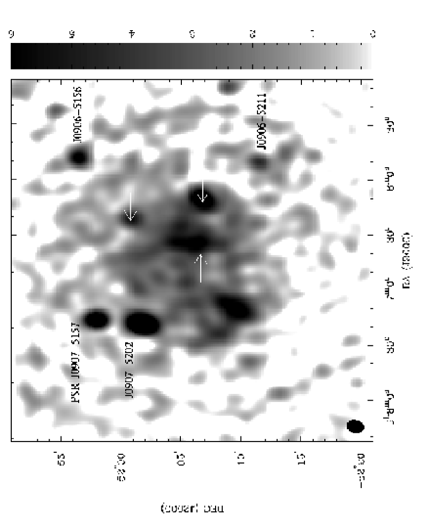
Figure 1: Radio image of G272.2$-$3.2 taken with the Australian Telescope Compact Array (ATCA) at 1.4 GHz. The optical filaments are indicated with by arrows. The positions of nearby pulsars are also indicated (Duncan et al. 1997).

G272.2$-$3.2 was discovered in the ROSAT All-Sky Survey (Greiner and Egger, 1993). It presents a centrally filled X-ray morphology and a thermally dominated X-ray spectrum. The temperature, as determined by the ROSAT PSPC observation is relatively high (between 1.0 and 1.5 keV for a 1$\sigma$ confidence level). No significant variation of the temperature could be measured with the X-ray data available from the ROSAT PSPC (Greiner, Egger, and Aschenbach, 1994).
Optical observations (Winkler and Hanson, 1993), made soon after the announcement of the discovery, confirm the nature of the nebulosity as a supernova remnant and the shock-heated nature of the emission. In particular, both the measured [Sii]/H$\alpha$ ratio and the detected emission from [Nii] 658.3-nm and [Oii] 732.5-nm are typical of SNRs. One of the fainter filaments is located at 09^h06^m40${}^{\rm s}\!.$4, -52^∘06^′42^′′ (J2000), about 1^′ north-west of the X-ray emission center. Brighter filaments with a similar [Sii]/H$\alpha$ are detected at 09^h06^m12${}^{\rm s}\!.$4, -52^∘06^′52^′′. There is no evidence for diffuse emission in the continuum images of the field.
Detailed radio observations (Duncan et al., 1997) have introduced a wealth of new data about this SNR. The radio observations were conducted at multiple frequencies and baselines using the Parkes radio telescope, the Australia Telescope Compact Array (ATCA) and the Molonglo Observatory Synthesis Telescope (MOST). G272.2$-$3.2 is of such low surface brightness ($\sim$ 1 mJy at 843 MHz) that even the sub-arcminute MOST observations could only map the brightest parts of the remnant. G272.2$-$3.2 presents an incoherent filamentary structure with diffuse, non-thermal emission of very low surface brightness as well as bright “blobs” which correlate well with the brightest optical filaments. This is a good indication that optical and radio emission emanate from the same regions. These regions are likely to be the ones where the shock interaction with the ISM is the strongest. We show in Fig. 1 a MOST radio image extracted from Duncan et al. (1997) on which the authors show the position of the optical filaments. There is no evidence for a clean “shell-like” morphology although the remnant is roughly circular with a 20^′ diameter and has a steep non-thermal radio spectral index (0.55$\pm$0.15), which is more typical of shell-like remnants than plerions. This implies that the diffuse emission detected within G272.2$-$3.2 is most probably due to shock-accelerated electrons. The spectral index varies relatively little across the remnant. There is no evidence of polarized emission from the remnant and Duncan et al. (1997) argue that this depolarization may be the result of turbulence occurring on angular scales of the order of 1^′. There is no evidence of pulsar-driven nebula.
There are data from the Infrared Astronomical Satellite (IRAS) survey at 12, 25, 60 and 100 $\mu$m. Infrared observations are unique in that they provide direct information on the dust present in the ISM and so they can serve as a powerful tool for temperature diagnostics. We have extracted the IRAS data at all four wavelengths and present our findings in the next section.
There are CO maps of the G272.2$-$3.2 sky region at a resolution of 18^′ (larger than the remnant). In this direction in the sky, velocity changes very little along the line of sight adding to the difficulty of constraining the distance to the remnant. The only significant CO emission is measured at velocities between -20 km s^-1 and 20 km s^-1 (T. Dame - private communication).
At a distance greater than 2 kpc, the large galactic latitude of G272.2$-$3.2 implies a distance below the plane larger than 110 pc. Using the distance distribution of SNRs in the Galaxy (Mihalas and Binney, 1981) and their galactic latitude (Green, 1998), we estimate that less than 10% of galactic SNRs are located at a greater distance from the plane. This results is in agreement with 100 pc upper limit given by Allen (1985) for the distance distribution of stars above the plane of the Galaxy and suggests a distance of about 2 kpc to G272.2$-$3.2.
This estimate, although solely based on a statistical analysis, turns out to be in good agreement with a value of $1.8^{\rm+1.4}_{\rm-0.8}$ kpc based on the measured X-ray column density of $N_{\rm H}=4.6\pm 3\times 10^{\rm 21}$atoms cm^-2 (Greiner, Egger, and Aschenbach, 1994). We also derive an estimate of an upper limit for the distance to the remnant. Using stars within a distance of 2 kpc, Lucke (1978) finds an optical color excess with distance of roughly 0.2 mag kpc^-1 in the direction of G272.2$-$3.2. Using the relation between color excess and column density ($N_{\rm H}=5.9\times 10^{\rm 21}\times E_{\rm{B-V}}$ atoms cm^-2) of Predehl and Schmitt (1995), one gets an upper limit of about 10 kpc for the distance to G272.2$-$3.2.
In view of all the uncertainties on the distance measurement, we adopt an “intermediate” distance scale of 5 kpc in the following computation and will examine the consequences of this estimate on the different dynamical states of the remnant. One must keep in mind that this value is mainly used as a scaling factor; we will keep the distance variation explicit in all our computations to allow easy computations at other distances of the physical quantities derived.

3 ASCA observations

3.1 Spatial Analysis

3.1.1 Images

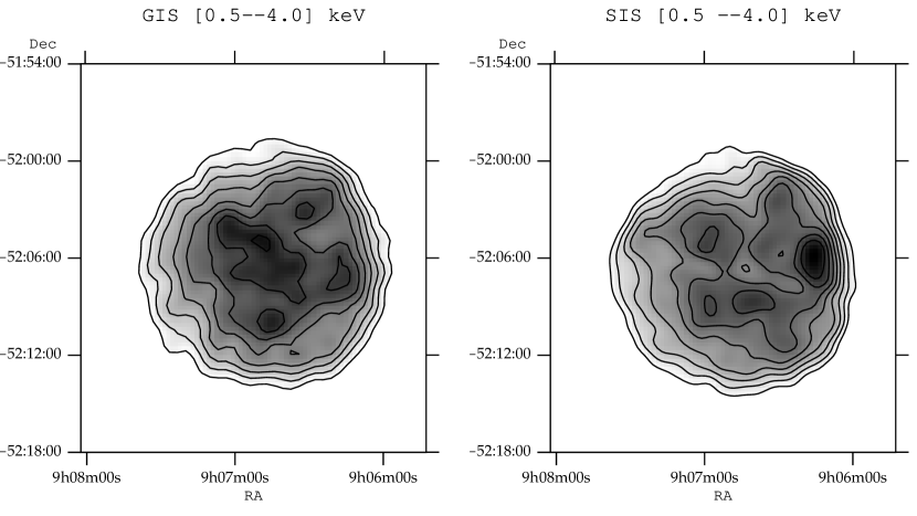
Figure 2: ASCA GIS(left) and SIS(right) images of G272.2$-$3.2 between 0.5 and 4.0 keV. Contour values are linearly spaced from 30% to 90% of the peak surface brightness in each map. Peak/Background values are (2.47/0.12) for the GIS and (3.20/0.19) for the SIS. All numbers are expressed in units of $10^{-3}$ counts s^-1 arcmin^-2.

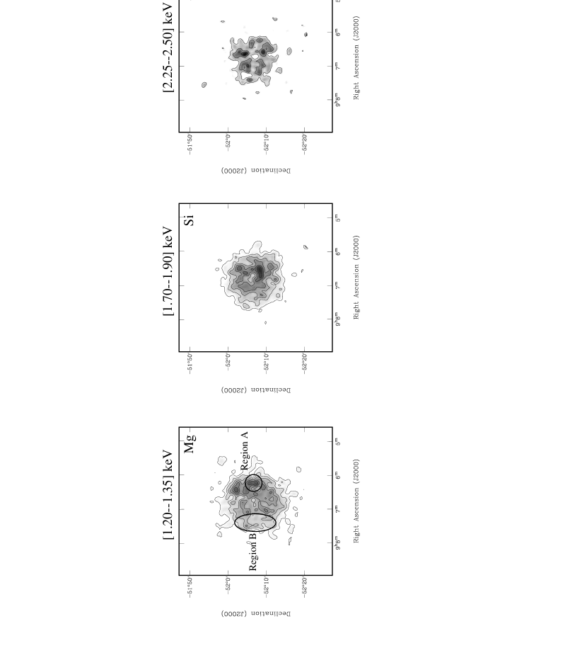
Figure 3: ASCA SIS images of G272.2$-$3.2 in three narrow band of energy. The energy band were chosen to isolate emission from Mg XI, Si XIII and S XV. We have indicated by a circle and an ellipse what is referred to as “region A” and “region B” in the analysis.

ASCA carried out one observation of G272.2$-$3.2 on 1995 January 20 at a nominal pointing direction of 09^h06^m43${}^{\rm s}\!.$2, -52^∘06^′14${}^{\prime\prime}\!.$4 (J2000). After applying the standard cuts on the data, we generated exposure-corrected, background-subtracted merged images of the GIS and SIS data in selected spectral bands. Background was determined from the weighted average of several nominally blank fields from high-galactic latitude observations with data selection criteria matched to those used for the SNR data. Exposure maps were generated from the off-axis effective-area calibrations, weighted by the appropriate observation time. Events from regions of the merged exposure map with less than 10% of the maximum exposure were ignored. Merged images of the source data, background, and exposure were smoothed with a Gaussian of $\sigma$= 30^′′ for both the low-energy band (0.5–4.0 keV) and the high-energy band (4.0–10.0 keV). We subtracted smoothed background maps from the data maps and divided by the corresponding exposure map. Fig. 2 shows the results obtained for the two detectors in the low energy band. The SNR is not detected above 4.0 keV and confirms the result from radio data that there is no sign of a pulsar-driven nebula. To examine the morphology of the remnant in more detail, we have generated SIS images in narrow energy bands in an attempt to isolate contributions from separate elements. We have minimized the continuum component by subtracting the average contribution from a small range of energy around each line imaged. In Fig. 3 we show SIS images of G272.2$-$3.2 in the three narrow energy bands [1.20 keV–1.35 keV], [1.70 keV–1.90 keV] and [2.25 keV–2.50 keV] corresponding to Mg XI, Si XIII, S XV lines respectively. The minimum visible in the center of all the images is due to an instrumental effect and corresponds to the location of the wide gap between CCDs in the SIS detector. There is a strong correlation between the Mg XI energy band map and the broad energy image. In the next section (spectral analysis) we will examine how this effect translates to a higher value of magnesium abundance inside the region of maximum emission.

3.1.2 Comparison with existing data

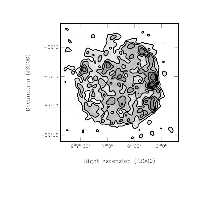
Figure 4: ROSAT HRI image of G272.2$-$3.2 after standard processing (Snowden et al. 1994).

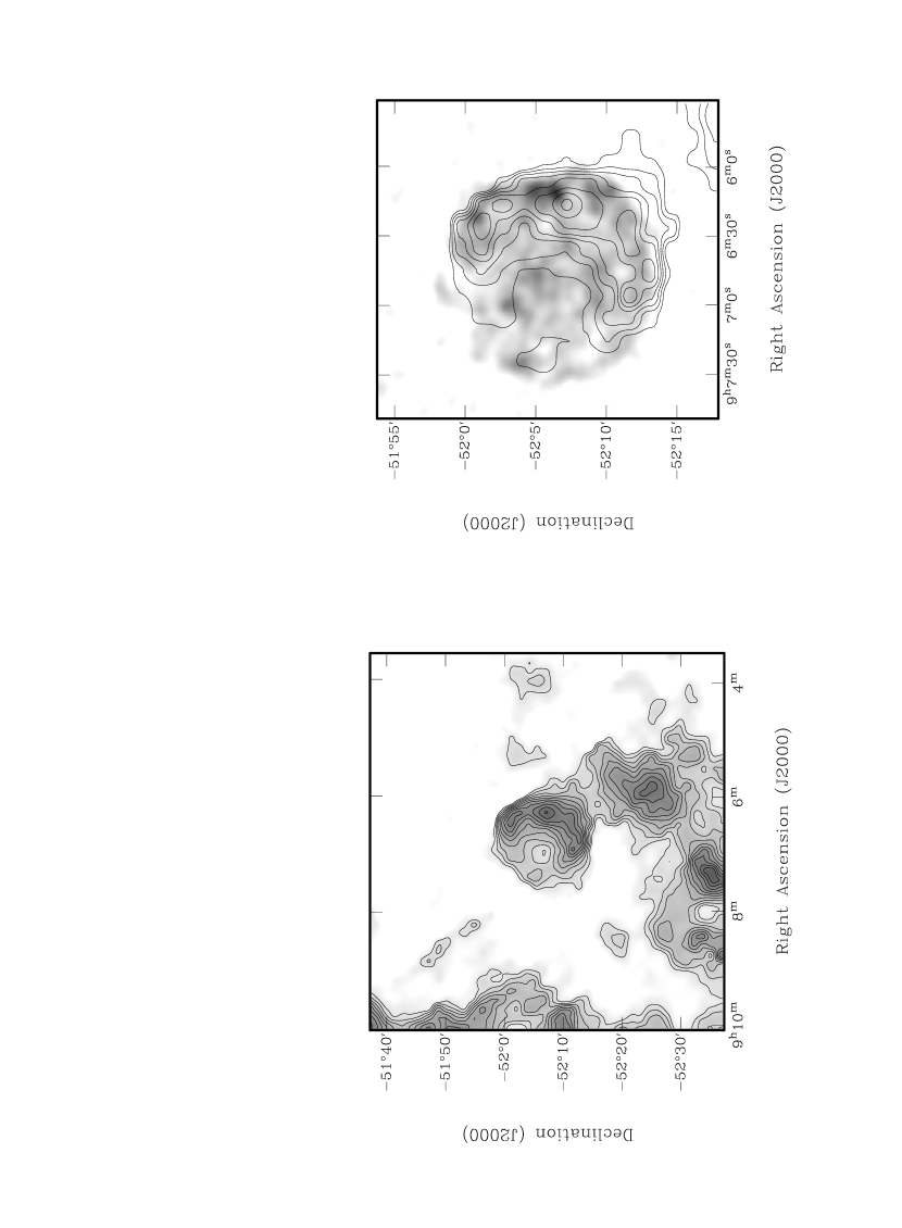
Figure 5: IRAS image of the 60$\mu$m/100$\mu$m emission for G272.2$-$3.2. (right) ROSAT HRI image superposed with contours from a close-up of the previous image.

To get yet a better estimate of the morphology of this remnant, we have analyzed ROSAT data from both the High Resolution Imager (HRI) and the Position Sensitive Proportional Counter (PSPC). Both sets of data were cleaned according to the standard prescription to study extended sources (Snowden et al., 1994). The software computes the contributions from the different backgrounds (solar scattered X-rays, high-energy particles, long and short term enhancements) and subtracts them from the data. Similar corrections are made for the HRI although contamination from those backgrounds is known with less accuracy. Fig. 4 shows the result of this procedure for the ROSAT HRI (the result is similar for the PSPC). A bright spot at the western edge of G272.2$-$3.2 is seen with a flattening of the shell at this location which coincides with the bright optical filament detected by Winkler and Hanson (1993). One explanation for this bright spot is that the expanding shock is encountering a density gradient in the local ISM. It could also well be that the shock has engulfed a cloud, slowed down, and that the cloud is being evaporated. At a distance of 5 kpc, the angular size of about 2^′25^′′ implies a cloud 3.5 pc in size. Using the results from the spectral analysis (see next section) we deduce a density between 0.42 and 0.70 cm^-3 for the clouds. The soft emission of that region is compatible with both explanations.
One useful indicator of the presence of dust in the galaxy is in the infrared energy band. Using data from the IRAS survey, Saken, Fesen and Shull (1992) studied the infrared emission from 161 galactic SNRs. They argue that young remnants tend to have strongest fluxes at 12$\mu$m and 25$\mu$m while somewhat older remnants have their strongest emission at longer wavelengths. G272.2$-$3.2 was not part of this study although its IRAS data show strong emission at 60 and 100$\mu$m (15 and 70 MJy str^-1 respectively) probably associated with the shock heated dust in the ISM. There is no significant emission at the two smallest wavelengths, a possible indication of a low dust temperature. One of the techniques commonly used to distinguish legitimate SNR emission from Hii regions and eliminate potential calibration or normalization problems, consists of studying the ratio of maps (60$\mu$m/100$\mu$m; 12$\mu$m/25$\mu$m) as an indicator of the respective contributions. This technique, applied with success for the Cygnus Loop (Saken, Fesen and Shull, 1992) has the advantage of being both simple and free from a lot of theoretical assumptions (about grain emissivities for example) that would otherwise complicate the interpretation.
We computed the ratio $F_{\rm 60}$/$F_{\rm 100}$ from the remnant (using the X-ray image to define its extent). We find that $F_{\rm 60}$/$F_{\rm 100}$ $\sim$ 0.2 which is comparable with what was measured for Vela XYZ (Saken, Fesen and Shull, 1992) but still lower than almost all the other ratios quoted (the highest being 2.45 for Kepler’s SNR). This low value of the $F_{\rm 60}$/$F_{\rm 100}$ emission is consistent with the low dust temperature hinted at by the lack of emission at 12$\mu$m and 25$\mu$m. Fig. 5 shows the smoothed (with a Gaussian of 3^′ ) image of the 60$\mu$m/100$\mu$m ratio and contours from a close-up of this image shown with the ROSAT HRI image superposed. The correlation with the brightest part of the SNR (the western part of the remnant) is obvious and in complete agreement with the optical, radio and X-ray data. It is remarkable not only that the SNR is so obviously detected in the IRAS data (and its very high background level), but that the agreement with the HRI image is so good. In the next section, we analyze spectra extracted from the brightest region and the rest of the remnant. The results from both spectral and spatial analysis are then used to form the global picture of the remnant.

3.2 Spectral Analysis

Depending on the age of G272.2$-$3.2 and on the pre-shock medium density, non-equilibrium ionization effects can become important (Itoh, 1979). In this case, a simple equilibrium collisional plasma emission model (Raymond & Smith 1977 – CEI model) can no longer be applied to reproduce the expected X-ray spectra. One has to take into account the fact that the ions are not instantaneously ionized to their equilibrium configuration at the temperature of the shock front. This model has, in addition to the temperature, an additional parameter which describes the state of the plasma ionization. This ionization state depends on the product of electron density and age and we define the ionization timescale as $\tau_{i}\equiv n_{e}t$. We have used an NEI model (Hughes and Helfand, 1985) keeping all the elemental abundances at their value given in Anders and Grevesse (1989) except when explicitly mentioned. In order to check the possibility of weak non-equilibrium ionization effects (for the dynamically older parts of the remnant), we have run both models (CEI and NEI) and compared the results from our spectral analysis.

3.2.1 Results from the Spectral Analysis

We have carried out several spectral analyses using the different data sets available and then combined them in order to obtain a general picture of the remnant. We have already seen that the remnant is undetected above 4 keV; all channels above that energy are ignored in the following analysis. After a first fit using only the ASCA data, we added data from the ROSAT PSPC to constrain $N_{\rm H}$, the value of absorption along the line of sight, using the cross-sections and abundances from Morrison & McCammon (1983). In all the analyses, the data were extracted from the ROSAT PSPC observation and then spatially matched to that of ASCA. We added a gain shift to both GIS 2 and GIS 3 (the same value for both detectors) according to the prescriptions from the calibration data analysis done by the ASCA-GIS team. An initial ASCA analysis was done on the complete remnant. We extracted a total of 25000 GIS events from a circular region encompassing the total emission region. The SIS was not used for the full SNR spectrum because the remnant covers more than one chip. We found that although it was impossible to describe accurately the complete SNR using a single model (CEI or NEI), the quality of the fit improves dramatically (from a $\chi^{2}$ of 870 to 514, for 325 degrees of freedom) in going from a CEI to an NEI model. We found a common gain shift (for both GIS 2 and 3) of -3.3% , consistent with the results found by the GIS calibration team.
The spectrum shown in Fig. 6 shows strong residuals at the silicon and sulfur energy lines. Neither the NEI nor the CEI can accurately model these two strong emission features.
In the next step of the analysis, we included data from the ROSAT PSPC data in the fit. In this case the column density is $N_{\rm H}=1.12\pm 0.02\times 10^{\rm 22}$ atoms cm^-2, the ionization timescale is $2150^{\rm+320}_{\rm-360}$ cm^-3 years, while the temperature is $kT=0.73^{\rm+0.03}_{\rm-0.04}$ keV (associated with a $\chi^{2}$/$\nu$ of 691.95/354). Both ionization timescale and the temperature of the plasma are compatible with the results found in the previous analysis but the column density is smaller. The total unabsorbed flux between 0.2 and 3.0 keV is $2.35\pm 0.15\times 10^{\rm-10}$ ergs cm^-2 s^-1. The fit for the complete remnant is shown in Fig. 6 and all the results are given in Table. 1. We note that the errors quoted for the measured parameters are underestimates in that they correspond to a fit with a large $\chi^{2}$/$\nu$.
In order to get a more quantitative picture of the remnant, we have separated it into “A” and “B”, two non-overlapping regions of emission. The “A” region is chosen to encompass the bright western part of the remnant (see Fig. 2 –left panel– or the following paragraph for a definition of the region) while the “B” spot is taken from the other region of the SNR, where no optical filaments have been observed.

3.2.2 Study of the “A” Region

We have extracted events from the “A” region defined in the ROSAT PSPC as a $\sim$ 2 ${}^{\prime}\mskip-5.0mu$ radius circle centered at 09^h06^m11${}^{\rm s}\!.$4, -52^∘05^′34${}^{\prime\prime}\!.$4 (J2000).
The same region is then selected for the ASCA SIS and GIS. Unfortunately the region is at the edge of the ASCA SIS and the circular region of extraction is truncated to take this into account. After background subtraction, the count rate is $0.084\pm 0.002$ cts s^-1, $0.024\pm 0.001$ cts s^-1, and $0.017\pm 0.001$ cts s^-1 in the ROSAT PSPC and ASCA SIS/GIS respectively (we have averaged the values for SIS 0 and SIS 1 as well as those for GIS 2 and GIS 3).
We model the five spectra using the NEI model mentioned above. As previously a gain shift is included in the analysis of GIS 2 and GIS 3 data.
The resulting $\chi^{2}$/$\nu$ is 248.35/133. All the results for region “A” are consistent with the ones found for the complete remnant when fit with a NEI thermal model. We find a column density of $N_{\rm H}=1.17^{\rm+0.02}_{\rm-0.06}\times 10^{\rm 22}$ atoms cm^-2, an ionization timescale of $760^{\rm+830}_{\rm-70}$ cm^-3 years and a temperature of $kT=0.86^{\rm+0.08}_{\rm-0.22}$ keV. We found a gain shift of -3% consistent with the results found previously (see results Table. 2a.). In comparison a fit using a CEI model (Mewe, Gronenschild and van den Oord, 1985; Mewe, Lemen and van den Oord, 1986; Kaastra, 1992), leads to a worse fit ($\chi^{2}_{\rm r}$ = 1.96). As we defined region “A” to be coincidental with the region of enhanced Mg X lines (see circle in Fig. 3), we added magnesium abundance as an extra parameter in the fit and check for any statistically significant drop in $\chi^{2}$. With this one extra parameter, the $\chi^{2}$/$\nu$ is now 176.07/129. The probability to exceed this value per chance is 0.003 compared to 5$\times 10^{\rm-9}$ for the previous fit. The column density is consistent with the previous result ($N_{\rm H}$ = $9.5^{\rm+0.7}_{\rm-1.0}\times 10^{\rm 21}$ atoms cm^-2), and so are the temperature ($kT=1.00^{\rm+0.35}_{\rm-0.08}$ keV) and the ionization timescale ($1385^{\rm+1860}_{\rm-550}$ cm^-3 years). The SIS detectors (the more sensitive instruments for measuring any abundance variation) do show a departure from the cosmic value (the smallest acceptable values range between 1.3 to 2 times solar abundance) but one has to keep in mind that the data were taken in a 4-CCD mode with degraded resolution and non-optimized calibration. All the other detectors yield spectra indistinguishable from models with cosmic values; the energy resolution of the ROSAT PSPC is too low to be sensitive to abundance variations, and both GIS spectra do show small indication of enhanced magnesium abundances, but the large $\chi^{2}$ resulting from the strong residuals at silicon and sulfur line energies renders it difficult to assess its significance (results are given in Table. 2b.).

3.2.3 Study of the “B” Region

We have carried out an identical analysis on the “B” region which, as mentioned above, designates the part of the remnant located at the other “edge” of G272.2$-$3.2. We extracted data from an ellipse of 2^′41^′′ and 5^′35^′′ minor and major axis, and located at 09^h07^m14${}^{\rm s}\!.$5, -52^∘06^′19${}^{\prime\prime}\!.$6 (J2000) (see Fig .3 – left panel).
This region selection allows us to study most of the emission within the remnant, but encompasses more than one CCD on the SIS detectors. The data from these detectors had to be combined prior to any analysis. As in the previous analysis, we used data from the ROSAT PSPC to constrain the value for the column density. After background subtraction, the count rates are $0.19\pm 0.003$ cts s^-1 for the ROSAT PSPC and $0.075\pm 0.001$ cts s^-1, and $0.066\pm 0.001$ cts s^-1 in ASCA SIS and GIS respectively.
We fit the data sets using an NEI model. Only the normalization varies from data set to data set. We applied a gain shift equal to that found in the previous analysis. We find ($\chi^{2}$/$\nu$= 635/317) a column density of $N_{\rm H}=1.30^{\rm+0.03}_{\rm-0.04}\times 10^{\rm 22}$ atoms cm^-2, associated with a temperature of $kT=0.65^{\rm+0.06}_{\rm-0.02}$ keV and an ionization timescale of $4180^{\rm+960}_{\rm-1290}$cm^-3 years (see Table. 3. for a summary).
From all the previous analysis, it seems possible to get a consistent description of the remnant. Both regions “A” and “B” have compatible temperature and ionization timescale. In the following section, we will examine what picture of the evolutionary state of the remnant these results imply.

3.3 Radial Temperature Gradient

One of the important goals of this work is to understand the origin of the centrally-peaked X-ray morphology of the remnant. The temperature profile is an important diagnostic tool to separate between models which can explain this kind of morphology. Some models, like a one-dimensional, spherically symmetric, hydrodynamic shock code (Hughes, Helfand, and Kahn, 1984), predict measurable variations of the observed temperature across the remnant, while others do not (White & Long 1991; hereafter WL). We have studied temperature variations across the remnant using data from the GIS 2. The remnant was separated in 5 annuli centered at 09^h06^m46^s, -52^∘06^′36${}^{\prime\prime}\!.$14 (J2000) chosen so as to contain the same number of events (around 3220 events) per annulus. We fixed the column density and the ionization timescale to the values found in the previous spectral analysis. All elemental abundances are kept linked to each other at their nominal ratio. This is only an approximation used to get an estimate of the possible temperature variation across the SNR. In the following section, we will examine both the temperature and surface brightness profile and consider two scenarios ( evaporation of cold clouds in the remnant interior and late-phase evolution incorporating the effects of thermal conduction) which have been applied to other remnants successfully to reproduce both the morphology and the temperature profile.

3.4 Radial profile of G272.2$-$3.2

3.4.1 Sedov-Taylor solution

In the soft X-ray band G272.2$-$3.2 is almost perfectly circular in appearance with a radius of $8^{\prime}$. As mentioned in the §2, the distance to G272.2$-$3.2 is not well known and its measured column density is large. In addition, there is no trace of any high-energy contribution from a central object. In this context, we have examined the possibility that G272.2$-$3.2 is a standard shell-like remnant which appears centrally peaked because of the large absorption along the line of sight or because of projection effects. If there were a density enhancement in the shell near the projected center of the remnant (due for example to the possible presence of metal-rich ejecta) that was similar to the density enhancement at the location of the shell toward the west, the remnant would have a centrally peaked morphology similar to the one observed. The fact that G272.2$-$3.2 presents both some limb brightening and centrally peaked emission could support this simple explanation. To quantify this model a little bit more we have studied the profile of G272.2$-$3.2 in the ROSAT HRI in 4 different quadrants of the remnant. We chose the quadrants so that the brightest part of the remnant (that we called region “A” in our spectral analysis ) belongs to one quadrant only. The profiles are shown in Fig. 7 and reveals the distinct enhancement on the west-side of the remnant. We have computed then the expected X-ray emission in the center for a simple shell model in which the inner radius is taken at 5 ${}^{\prime}\mskip-5.0mu$ (instead of the 7.4 ${}^{\prime}\mskip-5.0mu$ expected in the standard Sedov-Taylor solutions) to accommodate the measured west enhancement. We find that the central X-ray emission enhancement in the northern quadrant is a factor of 3 to 4 times brighter than expected from the shell at that position. This requires a density about a factor of two higher than in the shell, a factor not excluded by our analysis. In this case, the remnant evolution can simply be described by a set of Sedov-Taylor self-similar solutions.
The total X-ray emitting volume is $V=1.94\times 10^{59}\,f\,D_{\rm 5}^{\rm 3}$ $\theta_{\rm 8}^{\rm 3}$ cm³, where $f$ is the volume filling factor of the emitting gas within the SNR, $D_{\rm 5}$ is the distance to the remnant in units of 5 kpc, and $\theta_{\rm 8}$ the angular radius in units of 8${}^{\prime}\mskip-5.0mu$. In the following discussion, we have used the results of the NEI fit to the complete remnant (ASCA GIS and ROSAT-PSPC combined; see Table. 1.). Because of the relatively large value of the $\chi^{2}$ found in our best fit analysis, we have estimated physical parameters using a larger range of values than that found by the standard $\chi^{2}$ analysis and given in Table. 1 (we increased the errors by a factor 3). For an NEI normalization ranging from 3.2 to 4.1 $\times$ 10¹² cm^-5 and a ratio $n_{e}/n_{\rm H}$ between 1.039 and 1.084, we get a hydrogen number density $n_{\rm H}$ between 0.21 and 0.25 $\,D_{\rm 5}^{-1/2}\,\theta_{\rm 8}^{-3/2}\,f^{-1/2}$ cm^-3. The mass of X-ray emitting plasma $M_{X}$, in a Sedov-Taylor model, is between 35 and 184$\,D_{\rm 5}^{5/2}\,f^{1/2}\theta_{\rm 8}^{3/2}$ $M_{\odot}$. The estimated age of the remnant varies between 6250 and 15250 years and the initial supernova explosion ranges between 1.3 and 4.9 $\times 10^{\rm 50}\,D_{\rm 5}^{\rm 5/2}\,\theta_{\rm 8}^{\rm 3/2}\,f^{\rm-1/2}$ ergs. At a distance of 2 kpc (our lower limit on the distance), the emitting X-ray mass value is too small to allow for the remnant to have reached its Sedov-Taylor phase and the energy explosion is quite atypical of a supernova event.
As indicated in all the quantities derived, all these estimates have a strong dependence on the distance to the remnant. If the remnant is even further away than the distance derived by Greiner, Egger, and Aschenbach (1994), and this may well be the case, considering that the distance estimate used there is probably inaccurate by at least a factor 2, it is not impossible to reconcile the values deduced for both the emitting X-ray mass and the initial explosion energy with acceptable estimates for a standard SNR.

3.4.2 Cloudy ISM

Although it is possible that the centrally peaked X-ray morphology of G272.2$-$3.2 is due to the viewing effects mentioned in the previous section, we have examined other scenarios which could also explain it. In particular we have used a model (White and Long, 1991) based on cloud evaporation. This model invokes a multi-phase interstellar medium consisting of cool dense clouds embedded in a tenuous intercloud medium. The blast wave from the SN explosion propagates rapidly through the intercloud medium, engulfing the clouds in the process. In the model, these clouds are destroyed by gradually evaporating on a timescale set by the saturated conduction heating rate from the hot post-shock gas. Since this timescale can be long, it may be possible for cold clouds to survive until they are well behind the blast wave which, as they evaporate, can significantly enhance the X-ray emission from near the center of the remnant.
The timescale for cloud evaporation is one of the two extra parameters in the WL model added to the three of the standard Sedov solution: explosion energy $E_{0}$, ISM density $n$, and SNR age $t$. This timescale, which is expressed as a ratio of the evaporation timescale to the SNR age, $\tau_{e}\equiv t_{\rm evap}/t$, nominally depends on different factors, such as the composition of the clumps and the temperature behind the shock front, although such dependencies are not included explicitly in the model. The other extra parameter, $C$, represents the ratio of the mass in clouds to the mass in intercloud material. For appropriate choices of these parameters, the model can reproduce a centrally peaked X-ray emission morphology - see for example the application of this model to the centrally-peaked remnants W28 and 3C400.2 (Long et al., 1991). In the evaporating model atoms from the cold clouds enter the hot medium on timescales smaller than the ionization timescale. The line emission occurs after the ion has left the cloud and the ionization occurs in the hot phase. In this case, one would expect the highest ionized material to be near the center of the remnant or equivalently, to have the smallest range of ionization timescales further out. In all the following analysis, we have used emissivities derived from the NEI model with the ionization timescale fixed to the value from the complete remnant analysis.
We explored the parameter space of the two extra parameters and compare in Fig. 8 the results found for 3 representative sets of parameters with the HRI profile deduced for both the northern and western quadrants (as defined in Fig. 7). We also compared the expected temperature profile for the best value of $C$ and $\tau$ with the ASCA GIS measured temperature profile using an NEI model as described in Section 3.3. One can see that we can reproduce the emission weighted temperature variation across the remnant. The predicted profile agrees within the error bars with the emission profile from the most “centrally peaked” quadrant of the remnant but disagree with the profile extracted from the Western part of G272.2$-$3.2 (shown in dotted lines on Fig. 8). For comparison we have kept two other good trials for ($C$, $\tau$) equal to (50,20) and (35,10) respectively. The WL model allows for variations from the Sedov-Taylor in the physical quantities estimated from the spectral analysis but the differences stay small. For the values of ($C$=100,$\tau$=33) which provide an acceptable fit to the data, $M_{X}$ does not vary by more than 10% from the value derived in the Sedov-Taylor model.

3.4.3 Thermal conduction model

Thermal conduction is an alternative model to explain the morphology and emission from thermal composite remnants, and was used most notably for the SNR W44 [see Cox et al. (1999) for a detailed description of the model, and Shelton et al. (1999) for its application to W44]. It can be summarized as the first attempt to include classical thermal conduction in a fully-ionized plasma (Spitzer, 1956), moderated by saturation effects (Cowie and Mckee, 1977), to smooth the large temperature variations that are created in a Sedov-Taylor explosion. The result is a very flat temperature profile, dropping rapidly at the edge of the remnant.
We used odin, a one-dimensional hydrocode which includes the effects of non-equilibrium cooling and thermal conduction (Smith and Cox, 2000) to create models for a grid of explosion energies, ambient densities, and ages. SN explosion energies from $0.3-2\times 10^{\rm 51}$ ergs were considered along with ambient densities from 0.05-10 cm^-3, for ages in the range 2000-50,000 years. These give a range of remnant radii, X-ray spectra, and surface brightnesses that can be compared to the observed values for the remnant. As shown in Fig. 8, the best-fit temperature varies between 0.65-0.8 keV, and the surface brightness from $0.5-2.5\times 10^{\rm-3}$ cts s^-1 arcmin^-2 in the ASCA GIS. The average surface brightness is $\sim 10^{\rm-3}$ cts s^-1 arcmin^-2.
We found that low ($n_{0}\lesssim 0.5$ cm^-3) ambient densities were required in order to get a central temperature of 0.7 keV, just as was found in the Sedov-Taylor model. Higher densities led to lower temperatures (assuming a fixed surface brightness of $10^{\rm-3}$ cts s^-1 arcmin^-2), independent of the explosion energy. All other SNRs where the thermal composite model has been used successfully showed much higher ambient densities [4.72 cm^-3 for W44 (Shelton et al., 1999) and a best-fit density between 1-2 cm^-3 for MSH 11$-$61A (Slane et al., 2000)]. This low inferred density is a direct result of the high measured temperature, substantially larger than in those SNRs. In addition, the radial extent of the remnant on the sky is 8^′, so the physical radius is 11.6$D_{\rm 5}$ pc. The thermal conduction models we examined with the observed surface brightness and temperature require a minimum radius of 13.5 pc and age of 12,000 yr, suggesting a minimum distance of 5.8 kpc in the case of an explosion energy of $3\times 10^{\rm 50}$ ergs. A larger explosion energy will increase the radius and therefore the distance estimate.
We compared the observed GIS spectrum against solar-abundance NEI models from odin and the Raymond-Smith (Raymond and Smith, 1977) plasma model. Using the above-mentioned explosion parameters, the Sedov-Taylor swept-up mass is $\approx 120$M_⊙. The spectrum derived in this configuration leads to a reduced $\chi^{2}$ of 5.7 (assuming a column density of 1.3$\times 10^{\rm 22}$ atoms cm^-2). In addition, while the model matches the He-like magnesium lines at 1.4 keV, the model silicon emission at 1.8 keV is less than half the observed value, and the sulfur lines at 2.46 keV are far too weak. Using larger explosion energies only increases this trend in the models. This suggests that either the SNe that formed G272.2$-$3.2 had an atypically-small explosion energy, or that a thermal-conduction SNR model which does not include ejecta is not a good fit to the observations.

4 Discussion & Summary

G272.2$-$3.2 presents a couple of puzzles that we have addressed in this paper. First, the X-ray data point to a youngish remnant (its size – at the assumed distance of 5 kpc, its X-ray temperature, and the potential overabundance of Mg, Si and S) although its infrared emission resembles an older remnant profile. This lack of 12 $\mu$m and 25 $\mu$m emission could be due to a low dust density possible if the supernova explosion occurred in a cavity. Such a scenario would imply a massive progenitor (more than 8 to 10 M_⊙) with strong stellar winds, but is hard to combine with the model of a cloudy ISM put forward to explain the morphology. Note that according to nucleosynthesis models, a progenitor more massive than 15M_⊙ would yield more than 0.046, 0.071, and 0.023 M_⊙ of Mg, Si and S respectively (Thielemann, Nomoto and Hashimoto, 1996), which would require a swept-up mass of more than 100M_⊙ to lead to Mg and Si abundances less than twice that of cosmic abundances.
The radio morphology of G272.2$-$3.2 is difficult to characterize simply because of its low surface brightness which prevented a complete mapping of the remnant by the ACTA.
The X-ray peaked morphology can be explained by viewing effects or a cloud evaporation model. Both explanations provide reasonable estimates for the initial explosion energy and the total mass swept-up (depending here again on the distance estimate). A model involving thermal conduction, successfully applied to W44 (Shelton et al., 1999) requires the remnant to be around 5000 years old and associated with a low SN explosion energy. The model fails to reproduce the centrally peaked morphology of the remnant, consistent with G272.2$-$3.2 being too young for thermal conduction to have taken place.
The spectrum of the entire remnant presents evidence of strong lines (in the residuals of the ASCA GIS) which are not easily accounted for in the existing models (both CEI and NEI models). This could be a result of a a degraded response of the detectors, bad determination of the gain applied to the signal or the sign of something more fundamental, linked either to the simple models used or the properties of the remnant itself. We note that such strong lines are detected at the same energy range in at least two other remnants which present similar morphological characteristics: W44 (Harrus et al., 1997) and MSH 11$-$61A (Slane et al., 2000).
Because of the distance uncertainty, it is difficult to derive the initial parameters of the remnant (time and initial energy of the explosion). Low explosion energy supernovae do occur (see Mazzali et al. 1994 and Turatto et al. 1996 for the study of SN 1991bg) but this would be hard to reconcile with a massive progenitor scenario.
All these estimates are consistent with G272.2$-$3.2 being in the adiabatic phase of its expansion, but depend crucially upon the distance to the remnant. A better determination of this parameter would help characterize unambiguously the evolutionary state of G272.2$-$3.2 and will help further constrain the general picture of SNR’s evolution.

Figure 6: Spectra of the complete remnant for ROSAT PSPC and ASCA GIS. The two GIS detectors have been merged for display purposes only. The solid curves in the top panels show the best-fit NEI thermal plasma; the bottom panels plot the data/model residuals.

Figure 7: ROSAT HRI profile of the remnant extracted in 4 quadrants - We have chosen the cut so that region A , the region of bright optical filaments, fall into only one quadrant.

Figure 8: Radial temperature variation across the remnant (only up to the first five bins, representing the extent of the remnant) and the associated variation of the surface brightness. The temperature is measured using the ASCA GIS . The emission weighted temperature variation associated with the models is shown as well. The simulated profile is generated using ROSAT HRI. We have shown two extremes results: one obtained for the Northern quadrant (as defined in Fig. 7) shown in solid lines and one for the Western quadrant shown in dotted lines. We have shown the results from White & Long simulation using 3 different values of ($C$,$\tau$). Results for ($C$,$\tau$)=(100,33) are shown in solid lines. Dotted lines are for ($C$,$\tau$)=(50,20) and dashed lines are for ($C$,$\tau$)=(35,10). We have also indicated the range of normalization allowed by the error bars in the fit.

Table 1.

Results from the Spectral Analysis

Parameter Fit results Complete remnant (GIS and ROSAT PSPC), NEI thermal model^a $N_{\rm H}$ (atoms cm^-2) 1.12$\pm$0.02$\times$10²² $kT$ (keV) 0.73${}^{\rm+0.03}_{\rm-0.04}$ log($n_{e}t$) (cm^-3 s) 10.83${}^{\rm+0.06}_{\rm-0.08}$ Normalization(cm^-5)^b (3.5–3.8)$\times$10¹² Flux (ergs cm^-2 s^-1) ([ 0.2 – 3.0] keV) (2.2–2.5)$\times 10^{-10}$ Flux (ergs cm^-2 s^-1) ([ 3.0 – 10.0] keV) (4.3–4.6)$\times 10^{-13}$ Flux (ergs cm^-2 s^-1) ([ 0.4 – 2.4] keV) (2.0–2.3)$\times 10^{-10}$ $\chi^{2}$/$\nu$ 691.95/354 ^a Single-parameter 1 $\sigma$ errors ^b N=(${n_{\rm H}n_{e}V\over 4\pi D^{2}}$)

Table 2a. Region A, NEI thermal model Parameter Fit results $N_{\rm H}$ (atoms cm^-2) 1.17${}^{\rm+0.02}_{\rm-0.06}\times$10²² $kT$ (keV) 0.86${}^{\rm+0.08}_{\rm-0.22}$ log($n_{e}t$) (cm^-3 s) 10.38${}^{\rm+0.32}_{\rm-0.04}$ Normalization (cm^-5) (1.35–3.50)$\times$10¹¹ Flux (ergs cm^-2 s^-1) ([ 0.2 – 3.0] keV) (1.6–4.1)$\times 10^{-11}$ Flux (ergs cm^-2 s^-1) ([ 3.0 – 10.0] keV) (2.3–5.9)$\times 10^{-14}$ Flux (ergs cm^-2 s^-1) ([ 0.4 – 2.4] keV) (1.4–3.6)$\times 10^{-11}$ $\chi^{2}$/$\nu$ 248.35/133

Table 2b. Region A, NEI thermal model; Magnesium Abundance varies freely Parameter Fit results $N_{\rm H}$ (atoms cm^-2) 0.95${}^{\rm+0.07}_{\rm-0.10}\times$10²² $kT$ (keV) 1.00${}^{\rm+0.35}_{\rm-0.08}$ log($n_{e}t$) (cm^-3 s) 10.64${}^{\rm+0.37}_{\rm-0.22}$ Normalization (cm^-5) (0.6–1.9)$\times$10¹¹ [Mg]/[Mg]_⊙ (ROSAT; SIS 0&1; GIS 2&3) $0.5^{\rm+0.8}_{\rm-0.4}$ ;$2.2^{\rm+2.8}_{\rm-0.9}$; $2.7^{\rm+3.5}_{\rm-1.3}$; $1.4^{\rm+1.7}_{\rm-0.7}$; $1.2^{\rm+1.6}_{\rm-0.5}$ Flux (ergs cm^-2 s^-1) ([ 0.2 – 3.0] keV) (0.5–1.5)$\times 10^{-11}$ Flux (ergs cm^-2 s^-1) ([ 3.0 – 10.0] keV) (2.3–7.6)$\times 10^{-14}$ Flux (ergs cm^-2 s^-1) ([ 0.4 – 2.4] keV) (0.46–1.43)$\times 10^{-11}$ $\chi^{2}$/$\nu$ 176.1/129

Table 3. Region B, NEI thermal model Parameter Fit results $N_{\rm H}$ (atoms cm^-2) 1.30${}^{\rm+0.03}_{\rm-0.04}\times$10²² $kT$ (keV) $0.65^{\rm+0.06}_{\rm-0.02}$ log($n_{e}t$) (cm^-3 s) 11.11${}^{\rm+0.10}_{\rm-0.15}$ Normalization (cm^-5) (0.7–1.6)$\times$10¹² Flux (ergs cm^-2 s^-1) ([ 0.2 – 3.0] keV) (2.9–7.2)$\times 10^{-11}$ Flux (ergs cm^-2 s^-1) ([ 3.0 – 10.0] keV) (0.7–1.6)$\times 10^{-13}$ Flux (ergs cm^-2 s^-1) ([ 0.4 – 2.4] keV) (2.8–6.7)$\times 10^{-11}$ $\chi^{2}$/$\nu$ 635/317

References

- Allen (1985) Allen, C. W. 1985, Astrophysical Quantities, The Athlone Press, London
- Anders and Grevesse (1989) Anders, E., & Grevesse, N. 1989, Geochimica et Cosmochimica Acta, 53, 197
- Cowie and Mckee (1977) Cowie, L. L. & McKee, C. F. 1977, ApJ,211, 135
- Cox et al. (1999) Cox, D. P., Shelton, R. L., Maciejewski, W., Smith, R. K., Plewa, T., Pawl, A., and Rozyczka, M. 1999, ApJ, 524, 179
- Duncan et al. (1997) Duncan, A. R., Primas, F., Rebull, L. M., Boesgaard, A. M., Deliyannis, C. P., Hobbs, L. M., King, J. R., and Ryan, S. G. 1997, MNRAS, 289, 97
- Green (1998) Green, D. A. 1998, ‘A Catalogue of Galactic Supernova Remnants (1998 September version)’, Mullard Radio Astronomy Observatory, Cambridge, United Kingdom (available on the World-Wide-Web at “http://www.mrao.cam.ac.uk/surveys/snrs/”)
- Greiner and Egger (1993) Greiner, J. & Egger, R. 1993, IAU Circ No 5709
- Greiner, Egger, and Aschenbach (1994) Greiner, J., Egger, R., & Aschenbach, B. 1994, A & A, 286, L35
- Harrus et al. (1997) Harrus, I. M., Hughes, J. P., Singh, K. P., Koyama, K., & Asaoka, I. 1997, ApJ, 488, 781
- Hughes, Helfand, and Kahn (1984) Hughes, J. P., Helfand, D. J., & Kahn, S. M. 1984, ApJ, 281, L25
- Hughes and Helfand (1985) Hughes, J. P. & Helfand, D. J., 1985, ApJ, 291, 544
- Itoh (1979) Itoh, H. 1979, PASJ, 31, 541
- Kaastra (1992) Kaastra, J. S. 1992, An X-Ray Spectral Code for Optically Thin Plasmas, Internal SRON-Leiden Report, updated version 2.0
- Long et al. (1991) Long, K. S., Blair, W. P., Matsui, Y., & White, R. L. 1991, ApJ, 373, 567L
- Lucke (1978) Lucke, P. B. 1978, A&AS, 64, 367
- Mazzali et al. (1997) Mazzali, P. A., Chugai, N., Turatto, M., Lucy, L. B., Danziger, I. J., Cappellaro, E., della Valle, M., and Benetti, S. 1997, MNRAS, 284, 151
- Mewe, Gronenschild and van den Oord (1985) Mewe, R., Gronenschild, E. H. B. M., & van den Oord, G. H. J. 1985, A&AS, 62, 197
- Mewe, Lemen and van den Oord (1986) Mewe, R., Lemen, J. R., & van den Oord, G. H. J. 1986, A&AS, 65, 511
- Mihalas and Binney (1981) Mihalas, D., & Binney, J. 1981, Galactic Astronomy, W. H. Freeman and Cie, New York
- Morrison and McCammon (1983) Morrison, R., & McCammon, D. 1983, ApJ, 270, 119
- Predehl and Schmitt (1995) Predehl, P., & Schmitt, J. H. M. M. 1995, A&A, 293, 889
- Raymond and Smith (1977) Raymond, J. C., & Smith, B. W. 1977,ApJS, 35, 419
- Saken, Fesen and Shull (1992) Saken, J. M., Fesen, R. A. , & Shull, J. M. 1992,ApJS, 81, 715
- Sedov (1959) Sedov, L. I. 1959, Similarity and Dimensional Methods in Mechanics, (New York: Academic)
- Shelton et al. (1999) Shelton, R. A.,Cox, D. P., Maciejewski, W., Smith, R. K., Plewa, T., Pawl, A, and Rozyczka, M. 1999, ApJ, 524, 192
- Slane et al. (2000) Slane, P. O., et al. 2000, in preparation.
- Smith and Cox (2000) Smith, R. & Cox, D. 2000, ApJ, submitted
- Snowden et al. (1994) Snowden, S. L., McCammon, D., Burrows, D. N., & Mendenhall, J. A. 1994, ApJ, 424, 714
- Spitzer (1956) Spitzer, L. Jr. 1956, Physics of Fully Ionized Gases, (New York: Interscience), p. 87
- Taylor (1950) Taylor, G. I. 1950, Proc Royal Soc London, 201, 159
- Thielemann, Nomoto and Hashimoto (1996) Thielemann, F.-K., Nomoto, K., & Hashimoto, M. 1996,ApJ, 460, 408
- Turatto et al. (1996) Turatto, M., Benetti, S., Cappellaro, E., Danziger, I. J., della Valle, M., Gouiffes, C., Mazzali, P. A., and Patat, F. 1996, MNRAS, 283 , 1
- White and Long (1991) White, R. L., & Long, K. S. 1991, ApJ, 373, 543
- Winkler and Hanson (1993) Winkler, P. F., & Hanson, G. J. 1993, IAU Circ No. 5715