The Calar Alto Deep Imaging Survey:
$K$-band Galaxy Number Counts

We present $K$-band number counts for the faint galaxies in the Calar Alto Deep Imaging Survey (CADIS). We covered 4 CADIS fields, a total area of $0.2\,\mathrm{deg}^{2}$, in the broad band filters $B$, $R$ and $K$. We detect about 4000 galaxies in the $K$-band images, with a completeness limit of $K=19.75\,\mathrm{mag}$, and derive the $K$-band galaxy number counts in the range of $14.25<K<19.75\,\mathrm{mag}$. This is the largest medium deep $K$-band survey to date in this magnitude range. The $B$- and $R$-band number counts are also derived, down to completeness limits of $B=24.75\,\mathrm{mag}$ and $R=23.25\,\mathrm{mag}$. The $K$-selected galaxies in this magnitude range are of particular interest, since some medium deep near-infrared surveys have identified breaks of both the slope of the $K$-band number counts and the mean $B-K$ color at $K=17\sim 18\,\mathrm{mag}$. There is, however, a significant disagreement in the $K$-band number counts among the existing surveys. Our large near-infrared selected galaxy sample allows us to establish the presence of a clear break in the slope at $K=17.0\,\mathrm{mag}$ from $\mathrm{d}\log N/\mathrm{d}m=0.64$ at brighter magnitudes to $\mathrm{d}\log N/\mathrm{d}m=0.36$ at the fainter end. We construct no-evolution and passive evolution models, and find that the passive evolution model can simultaneously fit the $B$-, $R$- and $K$-band number counts well. The $B-K$ colors show a clear trend to bluer colors for $K>18\,\mathrm{mag}$. We also find that most of the $K=18-20\,\mathrm{mag}$ galaxies have a $B-K$ color bluer than the prediction of a no-evolution model for an $L_{*}$ Sbc galaxy, implying either significant evolution, even for massive galaxies, or the existence of an extra population of small galaxies.

1 Introduction

Many galaxy surveys have shown that galaxies were undergoing a significant evolution at intermediate redshifts ($0.5<z<1.0$). Cowie et al. (cow96 (1996)) and Ellis (ell97 (1997), et al. ell96 (1996)) suggested that an extra galaxy population in this redshift range is responsible for the excess of the galaxy number counts at faint magnitudes. With additional morphological classification for the faint galaxies, this extra population was identified as irregular and peculiar galaxies with strong star formation at intermediate redshifts (Glazebrook et al. gla95 (1995), Abraham et al. abr96 (1996), van den Bergh et al. vdb96 (1996), Huang et al. hua98 (1998)). The massive elliptical and giant spiral galaxies, however, show no significant evidence of evolution since $z=1.0$ (Lilly et al. lil95 (1995)).

As an indication that the faint blue galaxy excess has a significant contribution from galaxies at high redshift Cowie et al. (cow97 (1997)) find that at least some of their faint $B$-selected galaxies are located in a high-redshift ($1<z<2$) tail on the redshift distribution. Dickinson (dic00 (2000)) conducted a near-infrared study on HDF-N galaxies at using the NICMOS camera on HST and found far fewer high luminosity galaxies in the $1.4<z<2$ range. However, the NICMOS data cover only a small field, and may not be a representative sample. Steidel et al. (ste96 (1996),ste99 (1999)) have identified a large number of galaxies at higher redshifts ($z\sim 3-4$) using the Lyman-break technique. However, these galaxies do not contribute significantly to the faint blue galaxy number counts at $B<26\,\mathrm{mag}$. For $z>3$, the $B$ band covers wavelengths below the redshifted Lyman-alpha ($\lambda_{\mathrm{rest}}=1216\,$Å) line, where the rest-frame UV light is strongly affected by absorption in the Ly-$\alpha$ forest as well as dust.

Comparing the galaxy luminosity function at different redshifts is the most direct way of understanding the galaxy evolution. However existing samples are not large enough and the galaxy luminosity function at intermediate redshifts is not well determined (Lilly et al. lil95 (1995), Cowie et al. cow96 (1996), Ellis et al. ell96 (1996)), especially at lower luminosities. A wide field medium deep survey is required to obtain larger numbers of low luminosity galaxies, to better constrain the luminosity function at intermediate redshift. While large-format CCDs have been in use for some time now, sufficiently large near-infrared arrays have only recently become available.

There are three significant advantages to studying galaxy evolution in the near-infrared $K$ band instead of in the optical bands (Cowie et al. cow94 (1994), Huang et al. hua97 (1997)). First, the cosmological k-correction in the $K$-band is much smaller and better determined than the k-corrections in the optical bands. Second, the shorter wavelength optical bands sample restframe blue or UV light, and are thus very sensitive to the star-formation history in galaxies. Third, the $K$-band light is a close tracer of the stellar mass in galaxies, and less sensitive to either the star formation history or the galaxy spectral type. A $K$-selected sample of galaxies is thus more representative of the true distribution of galaxies.

A number of medium deep and deep $K$-band galaxy surveys have been conducted by various groups (Gardner et al. gar93 (1993), Songaila et al. son94 (1994), Djorgovski et al. djo95 (1995), Saracco et al. sar97 (1997, 1999), Minezaki et al. min98 (1998), Bershady et al. bers (1998), Moustakas et al. mou98 (1998) and Kümmel & Wagner kue (2000)). There is some disagreement between the $K$-band number counts of these surveys at faint magnitudes. Still, these surveys do show evidence for two critical phenomena which are important in understanding galaxy evolution: the mean $B-K$ color becomes bluer at faint magnitudes, and the slope of the $K$-band number counts shows a break in the $17<K<19$ magnitude range. The Hawaii $K$-band galaxy survey (Songaila et al. son94 (1994)) shows that galaxies in the range of $16<K<20$ magnitude are located at $0.3<z<1.3$, which spans an important epoch for galaxy evolution.

Table 1: Field coordinates

Field	$\alpha$(2000)	$\delta$(2000)	area [$\mathrm{arcmin}^{2}$]
01H	01:47:33.3	02:19:55	175
09H	09:13:47.5	46:14:20	127
16H	16:24:32.3	55:44:32	186
23H	23:15:46.9	11:17:00	188

To better determine the $K$-band number counts in this magnitude range, a $K$-band survey with much larger coverage is essential. Here, we use the Calar Alto Deep Imaging Survey (CADIS, Meisenheimer et al. mei99 (1998)) to derive improved $K$-band number counts in the range $14.25<K<19.75\,\mathrm{mag}$, as well as the corresponding optical number counts in the $B$ and $R$ bands. CADIS was originally tailored to search for Ly-$\alpha$ emitters at high redshift with Fabry-Perot Interferometer (FPI) imaging (Thommes et al. tho98 (1998)). However, the CADIS fields are also observed in three broad band filters ($B$, $R$, $J$ or $K$) and up to $13$ medium band filters with $\lambda/\Delta\lambda=25-50$. This multi-color database is also being used to study galaxy populations and their evolution at intermediate redshifts through their photometric redshifts (Wolf wo98 (1998)), as well as the detection of unusual objects like active galactic nuclei (Wolf et al. wo99 (1999)) and extremely red galaxies (Thompson et al. tho99 (1999)). Fried et al. (fried (2001)) present initial results from CADIS on the luminosity function of optically selected galaxies and their evolution.

In this paper, we present the optical and near-infrared galaxy number counts, as well as the colors of the $K$-selected galaxies. The four CADIS fields used for this study cover a total of 0.2 deg² down to a completeness limit of $K=19.75\,\mathrm{mag}$. Our coverage is four times the area of the ESO $K$-band survey (Saracco et al. sar97 (1997)), which is the largest medium deep $K$-band survey to date. The paper is organized as follows: The observation, data reduction and photometry are described in Section 2; the $B$-, $R$-, and $K$-band number counts are presented in Section 3, along with the colors of the $K$-selected galaxies. In Section 4 we present a galaxy model which reproduces the observed number counts, and Section 5 summarizes our results.

2 Observation and photometry

2.1 Observation and data reduction

Table 2: Observational parameters

	B			R			I		K
Field	Tel	Int	M90	Tel	Int	M90	Tel	Int	Tel	Int	M90
01H	2.2	5050	23.7	2.2	2800	22.8	2.2	4000	3.5	9648	19.4
09H	3.5	4000	24.9	2.2	2800	23.4	3.5	7000	3.5	11280	18.8
16H	2.2	6200	24.6	2.2	2500	23.7	2.2	13620	3.5	9067	19.3
23H	2.2	6230	23.4	2.2	2500	23.0	2.2	5000	3.5	6475	19.6

A complete description of the observation and data reduction for CADIS will be given elsewhere (Meisenheimer et al. in prep.), here we give only a brief description. The CADIS fields are selected at high galactic latitudes on the northern and equatorial sky. The two primary CADIS field selection criteria are: (1) no bright star ($R<16\,\mathrm{mag}$) within a field of 12’$\times$12’, and (2) a local minimum on the IRAS $100\,\mu m$ maps, with an absolute surface brightness of $<2\,\mathrm{MJy/sr}$. The field positions and areas covered in this project are given in Table 1.

The optical observations were obtained with focal reducing CCD cameras on the 2.2m and the 3.5m telescope on Calar Alto Spain. The Calar Alto Faint Object Spectrograph (CAFOS) covers a 200$\,\mathrm{arcmin}^{2}$ field at 0.53 arcsec per pixel on the 2.2 m telescope, while the Multi-Object Spectrograph for Calar Alto (MOSCA) covers a $150\,\mathrm{arcmin}^{2}$ at 0.33 arcsec per pixel on the 3.5 m telescope. Only images with seeing better than $1\aas@@fstack{\prime\prime}8$ are included in the CADIS database.

The $K$-band data were obtained with the Omega-Prime near-infrared camera (Bizenberger et al. biz98 (1998)) on the 3.5 m telescope at Calar Alto. Omega-Prime has a 1024$\times$1024 pixel HgCdTe array which, at 0.396 arcsec per pixel, covers a $6.8^{\prime}\times 6.8^{\prime}$ field of view. This camera has no cold pupil stop, which would effectively block thermal emission from the warm surface around the primary mirror. We used a $K^{\prime}$-filter (Wainscoat & Cowie wai92 (1992)) instead of the standard $K$-band to reduce the thermal background. In order to construct a larger field of view, matching that of the optical cameras, we observed the CADIS-fields in a $2\times 2$ mosaic. After trimming the high noise edges of the stacked mosaics, the final coverage for the $K$-band images varies from $127\,\mathrm{arcmin}^{2}$ to $188\,\mathrm{arcmin}^{2}$ (see Tables 1 and 2). The $K$ band image quality criterion is a seeing less than $1\aas@@fstack{\prime\prime}5$.

The optical images were initially processed using the Munich Image Data Analysis System (MIDAS) software package, while the near-infrared images were processed using the Interactive Data Language (IDL) or IRAF. Thompson et al. (tho99 (1999)) gives a discussion of the steps of the standard reduction to get the final, stacked images in the optical and the near-infrared. A detailed discussion on the detectability and photometry is given in the next section.

Photometric calibrations for all of the CADIS data are determined on the Vega scale. Each CADIS field has one or two relatively bright stars for which we have established accurate spectro-photometric calibrations between $350\,\mathrm{nm}$ and $950\,\mathrm{nm}$. The magnitudes of these tertiary standards are then obtained by integrating their spectral energy distributions within the CADIS filter profiles. Wolf (wo98 (1998)) gives a detailed description of the CADIS magnitude system and its calibration. For the $K$-band data, we use the UKIRT faint standard stars (Casali & Hawarden cas92 (1992)) for flux calibration. The total exposure times and detection limits for the optical and infrared data are given in Table 2.

We use the CADIS broad band $B$, $R$, and $K$ data for the number counts, and add the medium band $I$ ($\delta\lambda=25\,\mathrm{nm}$, centered at $815\,\mathrm{nm}$) data in order to facilitate star-galaxy separation. The CADIS B and R filters are very close to the Johnson-Cousins system ($B_{J}$ and $R_{kc}$ in the equations below). The transformations between the two systems were derived using synthetic photometry of the galaxy templates of Kinney et al. (kin (1996)) in the redshift range $0<z<1.5$. The transformation equations are:

$$B_{J}-B_{\mathrm{CADIS}}=0.082+0.121(B-R)_{\mathrm{CADIS}}$$ (1)

$$R_{kc}-R_{\mathrm{CADIS}}=-0.027-0.034(B-R)_{\mathrm{CADIS}}$$ (2)

2.2 Object detection and photometry

Object catalogs were created using the SExtractor image analysis package (Bertin & Arnouts ber96 (1996)). Before running the detection program, each image was convolved with a Gaussian PSF with a width equal to the full width at half maximum (FWHM) of the seeing. For detection, we required at least 5 connected pixels, each with a signal larger than three times the background noise. Faint galaxy detectability is determined using Monte Carlo simulations. Several bright galaxies with different morphological types were rescaled then added back into the original image before running the detection program again. The result is the percentage of galaxies recovered as a function of apparent magnitude. The magnitudes at which 90% of the test galaxies are recovered are listed in Table 2.

We used the photometry package MPIAPHOT (Meisenheimer & Röser mei86 (1986)), which was developed to measure accurate spectral energy distributions (SED) from images with variations in seeing. In MPIAPHOT, the pixel values within a circular aperture are evaluated using a Gaussian weighting function. The e-folding width $s_{w}$ of the Gaussian weighting function is set individually for each frame $i$ to

$$s_{w,i,x}=\sqrt{s_{\mathrm{eff}}^{2}-s^{2}_{i,x}}.$$ (3)

Here $s_{i}$ denotes the e-folding width of the seeing where $x=a,b$ corresponds to the major/minor axis of the empirical seeing profile and $s_{\mathrm{eff}}$ denotes the e-folding width of the effective PSF. The effective seeing is chosen as a constant for the dataset of every CADIS field, and compensates for variations in the seeing between images obtained at different times and through different filters. Since most of our images have a seeing of about $1\aas@@fstack{\prime\prime}5$ FWHM ($s_{i}=0\aas@@fstack{\prime\prime}90$) and the signal to noise ratio of the photometry has its maximum at $s_{\mathrm{eff}}\sim\sqrt{2}s_{i}$, the effective seeing is set to $s_{\mathrm{eff}}=1\aas@@fstack{\prime\prime}38$ for all data presented here.

The weighted pixel values are summed within an aperture of $4^{\prime\prime}$ diameter, and then corrected to a total magnitude. By default MPIAPHOT applies corrections calculated by integrating the flux of point-like objects to infinite radius. The corrected magnitude thus equals the total magnitude for point sources, but underestimates the total magnitude of extended galaxies. To correct for this effect, we apply another correction for galaxies. The corrections are determined from simulations containing galaxies which match the range of apparent sizes seen in the survey data. We find that the corrections for resolved galaxies are almost independent of the bulge to disk ratios and inclinations. The correction can be well described as a function of the measured size of the galaxies (i.e. the second moment along its major and minor axis) out to about $3^{\prime\prime}$ FWHM. The derived correction formula has been applied to the science data, in order to convert CADIS magnitudes to total magnitudes.

2.3 Star-Galaxy Separation

Figure 1: The color-color diagram for the $K$-selected sample. In the diagram, the dots represent the point-like objects and the crosses represent the extended objects. The solid line represents the empirical color criterion for star-galaxy separation (Cowie et al. cow94 (1994), Huang et al. hua97 (1997)).

Conventional star-galaxy separation is based on comparing the morphology of objects with the morphology of point-like objects. Since the $K$-images have the largest field size, there are regions where only information in $K$ is available, and there we used this conventional method for star-galaxy separation. However, this method fails to identify compact galaxies with unresolved morphology. While those objects are rare at bright magnitudes, this population amounts to $\sim 20\%$ of all galaxies at $R=23\,\mathrm{mag}$. To identify this population we use colors to separate stars and galaxies. In three fields presented here (01h, 09h and 16h field) the full CADIS dataset in broad bands and up to 13 medium band filters is available. In those fields the broad wavelength coverage from $0.4\,\mu\mathrm{m}$ to $2.2\,\mu\mathrm{m}$ allows a classification into stars, galaxies and QSOs based on the object’s SED. This is done by comparing the measured color indices of every object with the expected color indices calculated from template spectra of the different subclasses stars, galaxies and QSOs (Wolf wo98 (1998)). For galaxies and QSOs the theoretical color indices are calculated with a broad range of redshifts ($0<z<2$ for galaxies and $0<z<6$ for QSOs), the result of the classification includes a redshift estimate with an accuracy of typically $\delta z=0.03$ for galaxies (Fried et al. fried (2001)). For galaxies, we use the set of templates published by Kinney et al. (kin (1996)) whose SEDs range from an elliptical to an extreme starburst galaxy. This further allows a classification of the spectral type of galaxies found in the survey. For the 23h-field, for which we do not yet have the full color information, color-based classification was done using the color-color diagram $I-K$ vs. $B-I$ (Cowie et al. cow94 (1994), Huang et al. hua97 (1997)). To demonstrate this technique we plot in Fig. 1 the color-color diagram $I-K$ vs. $B-I$ of pointlike (dots) and extended (crosses) objects for the $K$-selected sample. In the $K$-selected sample stars and galaxies are well separated by the empirical relation

$$B-I=2.5*(I-K)-2$$ (4)

with only a few galaxies crossing the line.

To summarize the criterion for the final star-galaxy separation: an object is classified as a galaxy if either it is morphologically identified as a galaxy, or it is identified as a galaxy on the basis of its colors.

3 Optical and near-infrared galaxy number counts

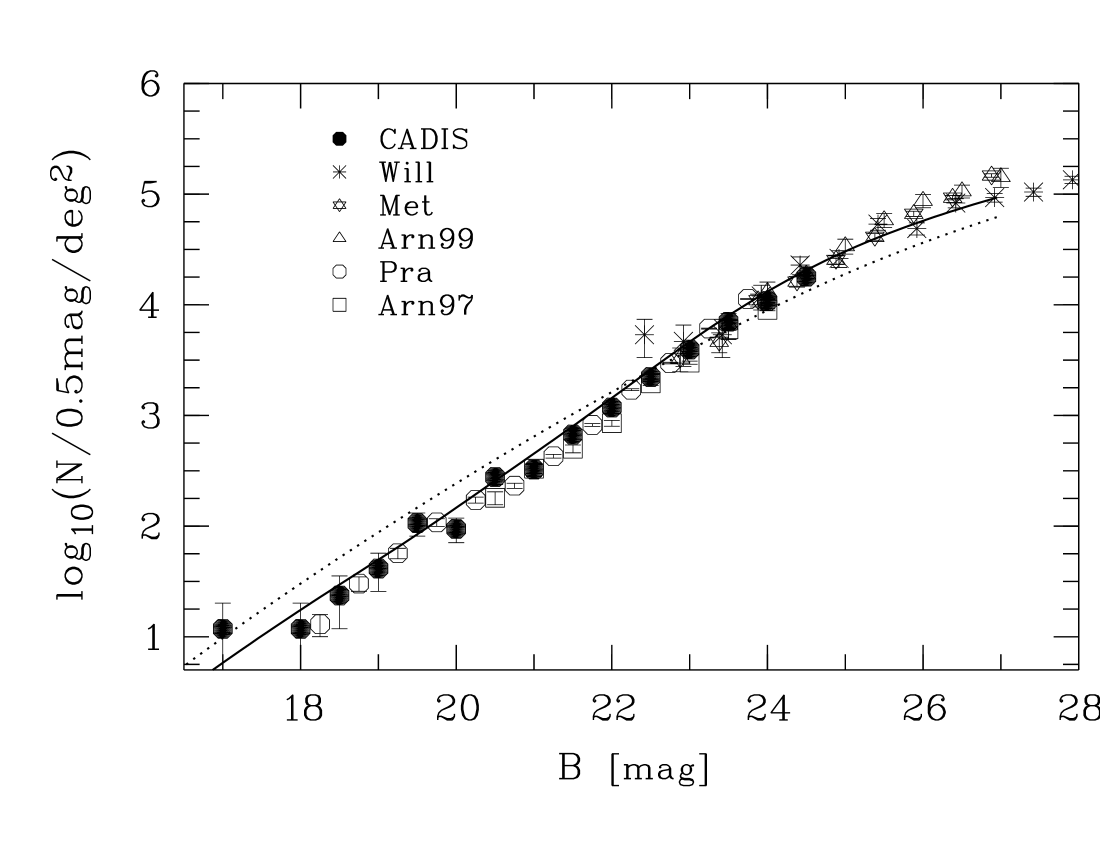
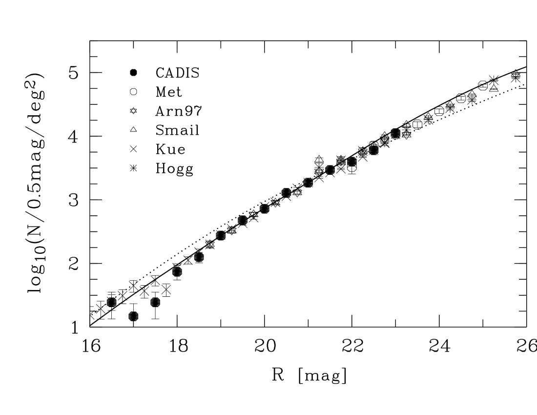
The galaxy number counts in the three filters are listed in Tables 3-5. The number counts in $B$ and $R$ are plotted in Figs. 2 and 3, respectively. We also compare our number counts to those of other large scale surveys with areas on a one square degree scale, like Arnouts et al. (arn97 (1997)), EIS (ESO Imaging Survey, Prandoni et al. pra (1999)) and Kümmel & Wagner (kue2 (2001)) and the deep surveys from Metcalfe et al. (met95 (1995)), Smail et al. (smail (1995)), the Hubble Deep Field (Williams et al. wil (1996)), Hogg et al. (hogg (1997)) and the NTT Deep Field (Arnouts et al. arn97 (1997)) In both filters there is a very good agreement between the CADIS data and the average literature counts over the entire magnitude range. Apart from serving as input for the models presented in the next section the agreement of our optical data with the literature confirm that the CADIS-fields contain the typical mix of galaxies, as it is expected for the wide field of view and the four lines of sight.

The CADIS $K$-band counts are plotted in Fig. 4. We also plot for comparison the results from other $K$-band surveys ( Gardner et al. gar93 (1993), Djorgovski et al. djo95 (1995), Gardner et al. gar96 (1996), Saracco et al. sar97 (1997), sar99 (1999), Huang et al. hua97 (1997), Minezaki et al. min98 (1998), Moustakas et al. mou98 (1998), Bershady et al. bers (1998), Szokoly et al., (szok (1999)), McCracken et al. mcc (2000) and Kümmel & Wagner kue (2000)). Because of the wide range in magnitudes covered by these surveys ($14<K<24$ mag), and the relatively small differences between them, we plot the $K$-band number counts in three magnitude ranges for better resolution.
At magnitudes brighter than $K=17.5\,\mathrm{mag}$, substantial $K$-band surveys with areas on the square-degree scale were carried out by Gardner et al. (gar96 (1996)), Huang et al. (hua97 (1997)), Szokoly et al. (1999) and Kümmel & Wagner (2000). Therefore, the number counts in this magnitude range are well defined. As shown in the up-left panel of Fig. 4, the CADIS $K$-band number counts in this magnitude range are in good agreement with previous number counts, but seem to support only the highest counts in the range $15.5<K<17.5\,\mathrm{mag}$

Figure 2: The $B$-band galaxy number counts. The filled circles are the number counts obtained in CADIS. The other symbols are number counts from Metcalfe et al. (met95 (1995)) (Met), Williams et al. (wil (1996)) (Will), Arnouts et al. (arn97 (1997)) (Arn97), Prandoni et al. (pra (1999)) (Pra) and Arnouts et al. (arn99 (1999)) (Arn99). The upper pair of lines show the passive evolution models, while the lower pair of lines show the no evolution models. In both cases, the solid lines are for $q_{0}=0.05$ while the dashed lines are for $q_{0}=0.5$ models.

In the magnitude range of $17.5<K<19.5\,\mathrm{mag}$ (upper right panel of Fig. 4) only the surveys of Minezaki et al. (min98 (1998), $181\,\mathrm{arcmin}^{2}$) and Saracco et al. (sar97 (1997), $170\,\mathrm{arcmin}^{2}$) have a coverage comparable to CADIS. With an area of $675\,\mathrm{arcmin}^{2}$ CADIS is the largest survey in this magnitude range. The CADIS counts are slightly lower than those of Minezaki et al. (min98 (1998)) at the faint end, but $50\,\%$ higher than the counts of Saracco et al. (sar97 (1997)) across the whole brightness interval. Because of the small statistical uncertainties due to the large $0.2\,\mathrm{deg}^{2}$ area of the four CADIS fields, our data provide a more robust measurement of the number counts in the range $16.5<K<19.5\,\mathrm{mag}$. The largest remaining discrepancies in the number counts are for $K>19.5\,\mathrm{mag}$, i.e. beyond the limit of the CADIS counts. At these faint magnitudes the scatter in the counts reach up to a factor of three (at $K\sim 21.0$, see lower left panel in Fig. 4). From the CADIS counts above the onset of this scatter at $K\geq 18\,\mathrm{mag}$, we conclude that CADIS favours the largest values obtained for the number counts at $K\geq 19\,\mathrm{mag}$, consistent with those obtained by Moustakas et al. (1997).

Magnitude errors, field-to-field variation and the Poisson noise are prime contributors to the uncertainties in the number counts. Fig. 4 shows in the lower right panel the number counts for the individual CADIS-fields. The differential counts for the individual fields give consistent results and therefore we exclude the possibility that the average number counts of all fields are affected by field to field variations. At $K>18\,\mathrm{mag}$ those variations can be significant only when the sky coverage of a survey is $\ll 100\,\mathrm{arcmin}^{2}$. Accordingly, the field-to-field variation and the Poisson noise may have significant contribution to the scatter of the $K$-band number counts among the deep surveys which cover only a small area on the order of $1\,\mathrm{arcmin}^{2}$.

In most cases, the uncertainties in the number counts result from systematic errors of the magnitude scale. As it is outlined in Huang et al.  (hua97 (1997)), a random magnitude error can cause the slope of the number counts to become steeper, while a systematic magnitude error can cause either a shift of number counts in the magnitude direction or change of the slope. The absolute CADIS-photometry (with respect to Vega) is accurate to $0.1\,\mathrm{mag}$ (Meisenheimer et al. in prep.). Taking into account those photometric errors leads to perfect agreement between our counts and the Minezaki et al. (1998) data, but even then the CADIS counts are still incompatible with the results of Saracco et al. (1997).

Figure 3: The $R$-band galaxy number counts. The filled circles are the number counts obtained in CADIS. The other symbols are number counts from Metcalfe et al. (met95 (1995)) (Met), Smail et al. (smail (1995)) (Smail), Arnouts et al. (arn97 (1997)) (Arn97), Hogg et al. (hogg (1997)) (Hogg) and Kümmel & Wagner (kue2 (2001)) (Kue). The models for the $R$-band number counts are plotted as in Fig. 2.

Figure 4: The $K$-band galaxy number counts. The filled circles are the number counts obtained in CADIS. The other symbols are number counts from Gardner et al. (gar93 (1993)) (Gar93), Djorgovski et al. djo95 (1995) (Djo), Gardner et al. (gar96 (1996)) (Gar96), Huang et al. (hua97 (1997)) (Huang97), Saracco et al. (sar97 (1997)) (Sar97), Minezaki et al. min98 (1998)) (Min), Moustakas et al. mou98 (1998) (Mou), Bershady et al. (bers (1998)) (Ber), Szokoly et al., (szok (1999)) (Szo), Saracco et al. (sar99 (1999)) (Sar99), McCracken et al. (mcc (2000)) (McCra) and Kümmel & Wagner (kue (2000)) (Kue). The models for the $K$-band number counts are plotted as in Fig. 2.

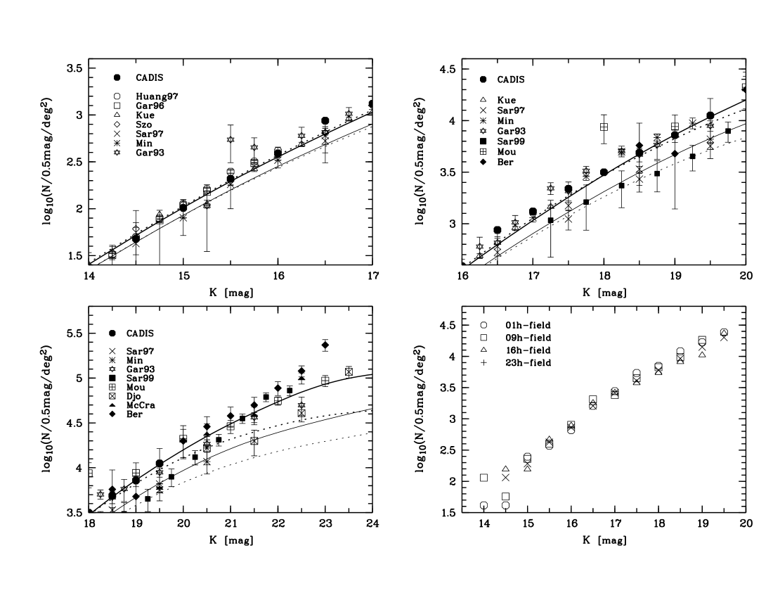
Gardner et al. (gar93 (1993)) reported finding a break in the logarithmic slope of the $K$-band counts at $K\sim 17$, where we have good statistics. To test for this, we fit a power law with the form $N(m)=a*10^{b*m}$ to our counts in various magnitude ranges. We find a clear break in $\mathrm{d}\log N/\mathrm{d}m$ from a bright-end slope of $b=0.64$ to a faint-end slope of $0.36$, with the break in the interval $16.5<K<17.0\,\mathrm{mag}$. The slope at the bright end is comparable to that found in other surveys (see Kümmel & Wagner kue (2000)). The slope at the faint end is somewhat steeper than values reported in the smaller surveys of Gardner et al. (gar93 (1993)) and Minezaki et al. (min98 (1998)), who give slopes around $0.24$.

Table 3: $B$-band number counts

B mag	Log(N)	Log(N-$\sigma$)	Log(N+$\sigma$)
17.0	1.07	0.54	1.30
18.0	1.07	0.54	1.30
18.5	1.37	1.07	1.55
19.0	1.62	1.41	1.76
19.5	2.03	1.91	2.12
20.0	1.97	1.85	2.07
20.5	2.44	2.37	2.50
21.0	2.51	2.45	2.57
21.5	2.83	2.79	2.87
22.0	3.07	3.04	3.10
22.5	3.35	3.32	3.37
23.0	3.60	3.58	3.61
23.5	3.85	3.83	3.86
24.0	4.03	4.02	4.05
24.5	4.25	4.24	4.27

Table 4: $R$-band number counts

R mag	Log(N)	Log(N-$\sigma$)	Log(N+$\sigma$)
16.0	0.69	0.15	0.99
16.5	1.39	1.13	1.55
17.0	1.17	0.79	1.36
17.5	1.39	1.13	1.55
18.0	1.87	1.74	1.96
18.5	2.10	2.01	2.18
19.0	2.44	2.38	2.50
19.5	2.68	2.63	2.72
20.0	2.86	2.82	2.89
20.5	3.11	3.08	3.13
21.0	3.27	3.25	3.30
21.5	3.47	3.45	3.49
22.0	3.60	3.59	3.62
22.5	3.78	3.77	3.80
23.0	4.05	4.04	4.06

Table 5: $K$-band number counts

K mag	Log(N)	Log(N-$\sigma$)	Log(N+$\sigma$)
14.0	1.21	0.83	1.40
14.5	1.68	1.51	1.81
15.0	2.01	1.90	2.10
15.5	2.32	2.25	2.39
16.0	2.59	2.51	2.62
16.5	2.94	2.91	2.97
17.0	3.12	3.09	3.14
17.5	3.34	3.32	3.36
18.0	3.50	3.48	3.51
18.5	3.69	3.68	3.70
19.0	3.86	3.85	3.87
19.5	4.05	4.04	4.06

Figure 5: The observed spectral type mix of galaxies (shaded) in the magnitude ranges close to the respective completeness limit in comparison to the predicted type-mix of the no-evolution and the passive-evolution model (the white and black bins, respectively).

4 Modeling the Number Counts and Galaxy Population

Models of galaxy number counts are primarily constrained by assumptions on the cosmological geometry, galaxy spectral evolution, and the galaxy luminosity function (see Gardner gardner98 (1998)). Theoretical uncertainties on the number count models come mainly from modeling the spectral evolution of galaxies, especially in the infrared bands. Many galaxy spectral synthesis models currently exist, ranging from simple stellar population models assuming an instantaneous burst of star formation to models including gas, recycling of metals, and nebular emission (Bruzual & Charlot bru93 (1993), Bertelli et al. bet94 (1994), Worthey wor94 (1994), Fioc & Rocca-Volmerange fio97 (1997)).

Most models make predictions consistent with each other at visible wavelengths (Charlot cha96 (1996)). There is, however, a significant scatter between model predictions at near-infrared wavelengths. This is due primarily to poor knowledge of the atmospheric parameters for cool stars and a substantial contribution from the nebular emission (Fioc & Rocca-Volmerange fio97 (1997)). Many number count models (Metcalfe et al. met96 (1996), McCracken et al. mcc (2000)) use simple stellar population models convolved with various star formation histories (Bruzual & Charlot bru93 (1993)), which over-predict the number counts at bright magnitudes at both visible and near-infrared wavelengths. We use PEGASE (Projet d’Etude des Galaxies par Synthese Evolutive), a new spectrophotometric evolution model which includes gas and dust components, nebular emission, and a better description of galaxy SEDs in the near-infrared (Fioc & Rocca-Volmerange fio97 (1997)). Our number count model constructed using PEGASE is able to fit the observed number counts at bright magnitudes well (Fioc & Rocca-Volmerange fio97 (1997)).

We adopt the passive evolution and no-evolution number counts models from Huang (hua97 (1997)). The cosmological k-correction and evolution e-correction are calculated using the PEGASE model. We plot model predictions against the observed number counts in Figs. 1-4. Huang (hua97 (1997)) has shown that these models correctly predict the surface density and color distribution of local galaxy populations, consistent with Fioc & Rocca-Volmerange (fio97 (1997)). The model Hubble types refer to the spectral type and not the morphological type, although they are correlated. The spectral types are defined by the e-folding time of the star formation rate. Most models use an exponentially decreasing star formation rate for all spectral types except Irr galaxies, which are so blue that the star formation rate must have been constant or increasing over the $\sim$4.5 Gyr life of the galaxy.

Figure 6: $B-K$ vs.  $K$ for the $K$-selected samples. The bright $K$-selected sample ($K<16\,\mathrm{mag}$) is obtained by Huang et al. (hua97 (1997)). The no-evolution and passive evolution models are plotted in separate panels. In each panel, the upper solid line is the $1.5\,L_{*}$ elliptical galaxy model; the middle line is the $L_{*}$ Sbc galaxy model; and the lower line is the $0.25\,L_{*}$ Sd/Irr galaxy model. The dashed lines link the colors among the different models at $z=0.5$ and $z=1.0$ (for $h_{0}=0.5$, $q_{0}=0.05$). Though the dashed lines are not exactly redshift contours, they roughly outline a redshift distribution on the color-magnitude relation. The cross is a medium $B-K$ color at each magnitude bin.

Figure 7: $R-K$ vs.  $K$ for the $K$-selected samples. The models and the medium colors are plotted in the same way as in Fig. 6.

We can see in Figs. 2-4 that evolution has the strongest effect on the models, while the geometry ($q_{0}=0.05$ and $0.5$) does not make a large contribution at brighter magnitudes ($B<24\,\mathrm{mag}$, $R<23\,\mathrm{mag}$ and $K<20\,\mathrm{mag}$). We adopt a high normalization of $\phi_{*}=0.02\,\mathrm{h}^{3}\mathrm{Mpc}^{-3}$. Only the passive evolution model is able to simultaneously fit the $B$-, $R$- and $K$-band number counts in a low density universe reasonably well. The no-evolution models are significantly flatter than the observational data. The $R$-band number counts show the highest excess and may favor an even higher normalization. The $K$-band counts have the lowest excess, but the no-evolution model still significantly under-predicts the counts for $K>16\,\mathrm{mag}$.

We note that Metcalfe et al. (met96 (1996)) and McCracken et al. (mcc (2000)) are able to fit their no-evolution model to the observed $K$-band number counts at faint magnitudes, while their passive evolution model predicts more galaxies than observed. This discrepancy between our model and theirs is due to the differences in the galaxy spectral evolution models in the $K$-band.

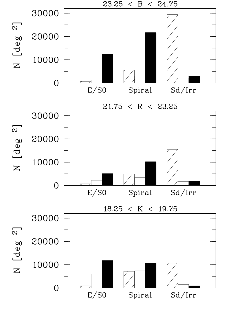
Although our passively evolving model is able to fit the observed number counts in the optical and near-infrared bands well, this does not necessarily mean that the passive evolution model is a correct physical description for galaxy evolution at intermediate redshifts. This is rather evident in Fig. 5 where we compare the spectral mix of our galaxies, as determined from their SEDs, with the predicted type mix from the no-evolution and the passive-evolution models. In all three bands this comparison is done in the $1.5\,\mathrm{mag}$ interval just brighter than the completeness limit of our data, where the statistics are best. The data and model predictions obviously disagree. The passive evolution model predicts that early type galaxies are mainly responsible for the excess over no-evolution model at faint magnitudes and high redshifts, Stellar evolution would make these early type galaxies much brighter at high redshifts because their stellar populations were younger. However, the spectral type mix of our number counts shows that even in the $K$-band spirals and SD/Irr are by far the main contributors to the counts. This can be understood if a population of star forming dwarf galaxies at $z<1.0$ dominates the number counts at faint magnitudes.

Another way of studying galaxy populations and their evolution is through color-magnitude diagrams. Fig. 6 ($B-K$ vs.  $K$) and Fig. 7 ($R-K$ vs.  $K$) are the color magnitude diagrams for the $K$-selected sample. The $B-K$ colors for the $K$-selected bright sample obtained by Huang (hua97 (1997)) are also plotted in Fig. 6. To compare with the data, we derived the $B-K$ and $R-K$ colors as a function of apparent magnitude $K$ for a $1.5\,L_{*}$ elliptical galaxy, a $L_{*}$ Sbc galaxy and a $0.25\,L_{*}$ Sd/Irr galaxy and plot them together with the observed color-magnitude data. Those three galaxy types have been used to calculate the model counts presented above, and they represent the populations with the reddest, medium, and bluest colors (the $B-K$ and $R-K$ colors at $z=0$ are given in Table 6). Provided the models accurately represent the color evolution of galaxies, the E and Sd/Irr model colors should bracket the observed distribution of colors and Sbc model colors trace the median of the color distribution. As seen in Fig. 6, the no-evolution and passive evolution models both bracket the $B-K$ color distribution at bright magnitudes very well, and both predict a break in the $B-K$ color at $K\sim 18\,\mathrm{mag}$. For the bright sample of Huang (hua97 (1997)), there is no significant difference between the no-evolution and passive evolution models. However, at $K>18\,\mathrm{mag}$ the non evolving Sd/Irr galaxy model colors are redder than a significant fraction of the observed colors. The passive evolution model predicts much bluer colors for these three types of galaxies at $K>18\,\mathrm{mag}$ and gives a better representation of the observed color distribution.

The dashed lines in Figs. 6 and 7 link the different models at $z=0.5$ and $z=1.0$ (for $h_{0}=0.5$, $q_{0}=0.05$). We can see why even the passive evolution model was unable to predict the type mix in Fig. 5: the ellipticals were brighter in the past and thus visible out to higher redshifts ($z>1$), making a significant contribution to the faint number counts. There are two obvious ways to explain this discrepancy between the observations and the models:
(i) Massive galaxies with high star formation rates at $z>1$ appear bluer and are accordingly classified as SED type later than E/S0, even though they will end up as early type galaxies at $z=0$.
(ii) less massive galaxies do not undergo significant star formation until relatively late times ($z<1$).
The good statistics from large galaxy samples and the spectral type studies favor the second alternative. However, it will be necessary to compare the model spectral type with the actual morphological Hubble type of the $K>18.0\,\mathrm{mag}$ galaxies before this question can be settled.

Table 6: Colors for E/S0, Sbc and Sd/Irr at z=0

	E/S0	Sbc	Sd/Irr
$B-K$	4.18	3.86	3.28
$R-K$	2.62	2.63	2.30

5 Summary

We derived the $B$-, $R$- and $K$-band number counts in the Calar Alto Deep Imaging Survey. The total coverage for the $K$-band imaging is about $0.2\,\mathrm{deg}^{2}$. The $B$-band number counts cover the range from $B=16.75\,\mathrm{mag}$ to $B=24.75\,\mathrm{mag}$; the $R$-band number counts cover from $R=15.75\,\mathrm{mag}$ to $R=23.25\,\mathrm{mag}$; and the $K$-band number counts cover from $K=13.75\,\mathrm{mag}$ to $K=19.75\,\mathrm{mag}$.
Our number counts at optical wavelength match the number counts of other surveys very well. Our $K$-band counts differ from the results of previous surveys by up to $50\,\%$. Because of the large area covered by our survey down to $K=19.75\,\mathrm{mag}$, the CADIS number counts in $K$ set a new standard in the range $17.75<K<19.75\,\mathrm{mag}$, where our survey represents the largest $K$-band survey to date. Between $K<16.5\,\mathrm{mag}$ and $K>17.5\,\mathrm{mag}$ our counts display a break in the logarithmic slope from $0.64$ to $0.36$, we estimate this break occurs around $K=16.7\,\mathrm{mag}$.

In order to get a first insight in the underlying evolution process we also adopt no-evolution and passive evolution models to fit our optical and near-infrared number counts. We find that both our optical and near-infrared number counts have an excess over the no-evolution model and can be simultaneously well fitted by the passive evolution model. The passive evolution model, however, predicts that the excess of the number counts at faint magnitudes is mainly due to the early type galaxies which were brighter at high redshifts. This is in contradiction to the observed spectral type mix contributions to our counts, which seems to be dominated by spirals and star-forming galaxies down to the faintest limits of our survey.
Thus we conclude that both non-evolving and passive evolution are both in contradiction with our observed number counts and the galaxy type mix at the faint magnitude end of our survey. The most sensible explanation for this finding would be a population at $z\leq 1.0$ with violent star burst events. These make them very prominent at intermediate redshifts while locally (at $z\sim 0$) they appear at such faint ends of both, the total luminosity and surface brightness range that they are underrepresented in current redshift surveys.

References

- (1) Abraham R.G., Tanvir N.R., Santiago B.X., et al., 1996, MNRAS, 279, L47
- (2) Arnouts S., de Lapparent V., Mathez G., et al., 1997, A&A Supl., 124, 163
- (3) Arnouts S., D’Odorico S., Cristiani S., et al., 1999, A&A, 341, 641
- (4) Bershady M.A., Lowenthal J.D., Koo D.C., 1998, ApJ, 505, 50
- (5) Bertin E., Arnouts S., 1996, A&A, 117, 393
- (6) Bertelli G., Bressan A., Chiosi C., Fagotto F., Nasi E., 1994, A&AS, 106, 275
- (7) Bizenberger P., McCaughrean M., Thompson D., Birk C., 1998, SPIE Conference Proceedings. vol. 3354, 109
- (8) Bruzual G., Charlot S. 1993, ApJ, 405, 538
- (9) Casali M.M., Hawarden T., 1992, JCMT UKIRT Newsletter, 4, 33
- (10) Charlot S., 1996, in From Stars to Galaxies: The Impact of Stellar Physics on Galaxy Evolution, ed. C. Leitherer, U. Fritze-von-Alvensleben, and J. Huchra, ASP Conference Series Vol. 98
- (11) Cowie L.L., Gardner J.P., Hu E.M., et al., 1994, ApJ, 434, 114
- (12) Cowie L.L., Songaila A., Hu E.M. Cohen J.G., 1996, AJ, 112, 839
- (13) Cowie L.L., Hu E.M., Songaila A., Egami, E., 1997, ApJ, 481, L9
- (14) Dickinson M., 2000, in Building Galaxies: From the Primordial Universe to the Present, ed. F. Hammer, T.X. Thuan, V. Cayatte, B. Guiderdoni, & J. Tranh Than Van, (Paris:Ed. Frontieres)
- (15) Djorgovski S., Soifer B.T., Pahre M.A., et al., 1995, ApJ, 438, L13
- (16) Ellis R.S., Colless M., Broadhurst T.J., Heyl J.S., Glazebrook K., 1996, MNRAS, 280, 235
- (17) Ellis R.S., 1997, ARAA, 35, 389
- (18) Fioc M., Rocca-Volmerange B., 1997, A&A, 326, 950
- (19) Fried J.W., von Kuhlmann B., Meisenheimer W., et al., 2001, A&A, accepted (astrph/0012343)
- (20) Gardner J.P., Sharples R.M., Carrasco B.E., Frenk C.S., 1996, MNRAS, 282, L1
- (21) Gardner J.P., 1998. PASP 110,291
- (22) Gardner J.P., Cowie L.L., Wainscoat R.J., 1993, ApJ, 415 L9
- (23) Glazebrook K., Ellis R.S., Santiago B.X., Griffiths R., 1995, MNRAS, 275, L19
- (24) Hogg D.W., Pahre M.A., McCarthy J.K., et al., 1997, MNRAS 288, 404
- (25) Huang J.-S., Cowie L.L., Gardner J.P., et al., 1997, ApJ, 476, 12
- (26) Huang J.-S., 1997, Ph.D. Thesis, University of Hawaii
- (27) Huang J.-S., Cowie L.L., Luppino G.A., 1998, ApJ, 496, 31
- (28) Kinney A.L., Calzetti D.A., Bohlin R.C., et al., 1996, ApJ, 467, 38
- (29) Kümmel M.W., Wagner S.J., 2000, A&A, 353, 867
- (30) Kümmel M.W., Wagner S.J., 2001, A&A, submitted
- (31) Lilly S.J., Tresse L., Hammer F., Crampton D., LeFèvre O., 1995, ApJ, 455, 108
- (32) McCracken H.J., Metcalfe N., Shanks T., et al., 2000, MNRAS, 311, 707
- (33) Meisenheimer K., Röser H.-J., 1986, in The Optimization of the Use of CCD Detektors in Astronomy, ed. J.-P. Baluteau & S. D’Odorico (Munich:ESO-OHP), 227
- (34) Meisenheimer K., Beckwith S., Fockenbrock R., et al., 1998, in ASP Conf. Ser. 146, in The Young Universe, ed S. D’Odorico, A. Fontana, & E. Giallongo (San Francisco:ASP), 134
- (35) Metcalfe N., Shanks I., Fong R., Roche N., 1995, MNRAS, 273, 257
- (36) Metcalfe N., Shanks I., Campos R., Fong R., Gardner J. P., 1996, Nature, 383, 236
- (37) Minezaki T., Kobayashii Y., Yoshii Y., Peterson B.A., 1998, ApJ, 494, 111
- (38) Moustakas L.A., Davis M., Graham J.R., et al., 1997, ApJ, 475, 445
- (39) Prandoni I., Wichmann R., da Costa L., et al., 1999, A&A, 345, 448
- (40) Saracco P., Iovino A., Garilli B., Maccagni D., Chincarini, C., 1997, AJ, 114, 887
- (41) Saracco P., D’Odorico S., Moorwood A., et al, 1999, A&A, 349, 751
- (42) Smail I., Hogg D.W., Yan L., Cohen J.G., 1995, ApJ 449, L105
- (43) Songaila A., Cowie L.L., Hu E.M., Gardner J.P., 1994, ApJS, 94, 461
- (44) Steidel, C. C., Giavalisco, M., Petini, M., Dickinson, M., Adelberger, K. L., 1996 ApJ, 462, L17
- (45) Steidel, C. C., Adelberger, K. L., Giavalisco, M., Dickinson, M., Petini, M., 1999, ApJ, 519, 1
- (46) Szokoly G.P., Subbarao M.U., Connolly A.J., Mobasher B., 1999, ApJ, 492, 452
- (47) Thommes E., Meisenheimer,K., Fockenbrock R., et al., 1998, MNRAS, 293, L6
- (48) Thompson D., Beckwith S.V.W., Fockenbrock R., et al., 1999, ApJ, 523, 100
- (49) van den Bergh S., Abraham R.G., Ellis R.S., et al., 1996, AJ, 112, 359
- (50) Wainscoat R.J., Cowie L.L., 1992, AJ, 103, 332
- (51) Williams R.E., Blacker B., Dickinson M., et al., 1996, AJ 112, 1335
- (52) Worthy G., 1994, ApJS, 101, 181
- (53) Wolf C., 1998, Ph.D. Thesis, University of Heidelberg
- (54) Wolf C., Mundt R., Thompson D., et al., 1999, A&A, 343, 399