N-Body Simulations of Open, Self-Gravitating Systems

Abstract

Astrophysical systems differ often in two points from classical thermodynamical systems: 1.) They are open and 2.) gravity is a dominant factor. Both modifies the homogeneous equilibrium structure, known from classical thermodynamics. In order to study the consequence for structure formation in astrophysical systems, we carry out N-body simulations of self-gravitating systems, subjected to an energy-flow. The simulations show that physically realistic, time-dependent boundary conditions can maintain a molecular cloud in a statistically steady state, out of thermodynamic equilibrium.

Moreover we perform some simple “gravo-thermal” N-body experiments and compare them with theoretical results. We find negative specific heat in an energy range predicted by [*]authorf:Follana99.

1 Introduction

An energy-flow through a system is related to an entropy-flow. If the entropy-flow leaving the system is larger than those entering, then the system evacuates it’s internal, by irreversible processes produced entropy to the outer world. Consequently order is created inside the system, which diverges from a classical thermodynamical equilibrium in a closed system. Far from equilibrium, the system is no longer characterized by an extremum principle, thus losing it’s stability. Therefore perturbations can lead to long range order, through which the system acts as a whole. Such a behavior is well known in laboratory hydrodynamics and chemistry. The underlying concepts such as “dissipative structures” and “self-organization” were extensively studied (see e.g. [Nicolis & Prigogine1977]). But despite of their popularity they are until now only little studied in the context of non-equilibrium structures in self-gravitating astrophysical systems. Therefore we take up some ideas of these concepts and build a simple model of an open self-gravitating system. With this model we want to check if an energy-flow can maintain a self-gravitating system in an statistically stable state, out of thermodynamical equilibrium and if gravitation in combination with an energy flow can create structures with a higher degree of order.

The simplicity of the model permits, furthermore, to perform some “gravo-thermal” experiments whose results can be compared with theory.

2 Why Dissipative N-Body Systems?

The use of hydrodynamics to simulate self-gravitating, clumpy gas may be problematic, due to the following reasons:

1.) During recent years observations revealed that molecular clouds are structured down to the smallest resolvable scales. These structures appear fractal. As a consequence density, temperature and related fields are not everywhere differentiable, rendering the use of hydrodynamics problematic.

2.) Hydrodynamics is based on the assumption of a local thermodynamic equilibrium (LTE). But such an equilibrium may not be established in gravitationally unstable media because the speed of matter disturbances is comparable to the sound speed ([Pfenniger1998]).

3.) Thermodynamical formalism incorporating gravity yield results differing from those of classical thermodynamics. An example of this is the so called gravo-thermal catastrophe. The application of these formalism lead among other things to spatially inhomogeneous equilibrium states. In hydrodynamics gravity is inserted in the Euler equation as an external force. But the thermodynamical variables are determined by a theory not taking gravity into account. Because gravity can change thermodynamical behavior, it is not a priori clear that hydrodynamical methods can simulate self-gravitating gas correctly.

Bearing in mind these considerations we try an other approach in order to model self-gravitating interstellar gas. That is, we use dissipative particles, representing dense cloud fragments, to simulate cosmic gas ([Huber & Pfenniger2001a]).

Furthermore, with such a realization we can check some thermodynamic results of self-gravitating systems with softened potentials.

3 Model

3.1 Principle

To prevent gravitationally unbound particles from dissolution, the particles are confined in a spherical potential well. This prevents a matter flow. However, our system is subjected to an energy flow. This flow is maintained by energy injection (heating) and dissipation. The energy is injected due to time and space dependent potential perturbations. The dissipation is realized by a local or global cooling scheme.

Among others we apply a particle potential becoming repulsive on the softening length scale. With such a potential we want to prevent the formation of very dense particle agglomerates below the resolution scale. The repulsive force is analogous to the molecular van der Waals force.

3.2 Self-Gravity and Repulsion

The gravitational forces are computed on the Gravitor Beowulf Cluster with a parallel tree code, based on the [*]authorf:Barnes86 tree algorithm. The particle potential is:

$$\Phi_{\rm p}(r)=-\frac{Gm}{\sqrt{r^{2}+\epsilon^{2}}}\left(1-\xi\frac{\epsilon^{2}}{(r^{2}+\epsilon^{2})}\right)\;,$$ (1)

where $m$ is the particle mass, $\epsilon$ is the softening length and $r$ is the distance from the particle center. The parameter $\xi$ determines the deviation from the Plummer potential $\Phi_{\rm Pl}$. The potential is repulsive for $\xi>1/3$ in the range $|r|<\epsilon\sqrt{(}3\xi-1)$ (see Figure 1).

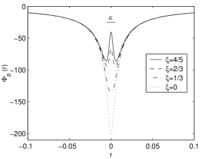
Figure 1: The potential as a function of $r$ in units of $Gm/R$, where $m$ is the particle mass. For $\xi>1/3$ the potential is repulsive on the softening length scale.

3.3 Confinement

The confinement potential, preventing the dissolution of gravitationally unbound particles has the form,

$$\Phi_{\rm conf}\propto R^{16}\;,$$ (2)

where $R$ is the distance from the center of the system.

3.4 Perturbation (Heating Scheme)

The energy injection is due to time-dependent boundary conditions or more precise due to a perturbation potential. The perturbation potential is shown in Figure 2. The amplitude and the frequency can be controlled by parameters. If our system represents a molecular cloud then potential perturbations can be due to star clusters, clouds or other high mass objects passing in the vicinity. Indeed such stochastic encounters must be quite frequent in galactic disks and we assume,

$$\frac{1}{f_{\rm pert}}\ga\tau_{\rm dyn}\;,$$ (3)

where $f_{\rm pert}$ is the mean frequency of the encounters. Thus these encounters can provide a continuous low frequency energy injection on large scales.

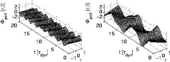
Figure 2: Perturbation potentials as a function of time and 1D-space. The space coordinate r is determined through $r^{2}=x^{2}+y^{2}+z^{2}$ and $x=y=z$. The time is indicated in units of dynamical times. We show two perturbation potentials with different frequency and amplitude. Full resolution version of this figure is available at: http://obswww.unige.ch/Preprints/dyn_art.html

3.5 Energy Dissipation

In order to maintain an energy-flow we must dissipate somehow the energy injected at large scales. We use two different dissipation schemes.

1. Local Dissipation

A particle dissipates energy during an “inelastic encounter” with an other particle. Thus we add friction forces, depending on the relative particle velocities $\vec{V}$ and positions $\vec{r}$. The friction forces are:

$$F_{i}\propto\left\{\begin{array}[]{rcl}\frac{V\cos\vartheta}{r}e_{i}&:&r>\lambda\epsilon\\ 0&:&r<\lambda\epsilon\end{array}\right.\;,$$ (4)

where $Vr\cos\vartheta=\vec{V}\vec{r},\;i=\{x,y,z\}$, $\vec{e}$ is the unity vector $\vec{V}/V$ and $\lambda$ is a parameter $>1$ ensuring the local nature of the dissipation.

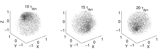
Figure 3: A self-gravitating system subjected to an energy-flow. The energy-injection compensates the dissipated energy and a statistically steady state is reached.

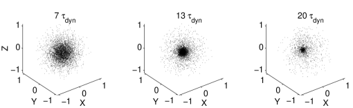
Figure 4: The evolution of a self-gravitating system with local dissipation, but without heating, i.e., without energy-flow.

2. Global Dissipation

The global dissipation term depends not on the relative velocity $\vec{V}$ but on the absolute velocity $\vec{v}$. The global friction force, causing an energy dissipation is: $F_{i}\propto-v_{i}$.

4 Results

We present here some preliminary results of a paper in preparation ([Huber & Pfenniger2001b]).

4.1 Self-Gravity and Energy Flow

With an appropriate tuning of the energy injection we can prevent the collapse of a self-gravitating dissipative system and maintain it in a statistically steady state out of thermodynamic equilibrium. This is shown in Figure 3. The system subjected to an energy flow attains a statistically steady state after about $10\>\tau_{\rm dyn}$. The evolution of the same system, but without energy injection, is shown in Figure 4. Both simulations were carried out with a local dissipation scheme and 10000 particles, from which 5000 are shown.

The system subjected to an energy-flow is not thermalized. A temperature gradient arises, in such a way that a cooler mass condensation is embedded in hotter shells (see Figure 5). Such temperature gradients are typical for molecular clouds.

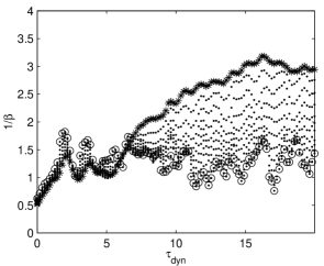
Figure 5: The evolution of the Lagrangian temperature of the system shown in Figure 3. $\beta$ is the inverse dimensionless temperature $(\beta=1/T)$. Each curve depicts the temperature of a mass fraction, contained in a sphere. The mass spheres are centered at the center of mass and the corresponding mass fractions are: $\Delta M/M=\{5\%,10\%,20\%,\ldots,80\%,90\%,98\%\}$. Circles: $\Delta M/M=5\%$. Crosses: $\Delta M/M=98\%$.

We checked the model behavior in dependence of the different particle potentials, heating and cooling parameters. Actually we find statistically stable states, but these states are not endowed with higher degrees of order.

5 Gravothermal experiments

If we switch off the heating process and use a global dissipation scheme we can cool the system and maintain it nearly in thermodynamic equilibrium. Thus we can perform some simple “thermodynamic experiments” of self-gravitating N-body systems. Follana & Laliena examined the thermodynamics of self-gravitating systems with softened potentials. They achieve a softening by truncating to $n$ terms an expansion of the Newtonian potential in spherical Bessel functions (we will call this potential hereafter Follana potential). This regularization allows the calculation of the thermodynamical quantities of self-gravitating systems. The form of their potential is similar to a Plummer potential with a corresponding softening length (see Figure 6). Thus we can check their theoretical results by using a Plummer softened potential.

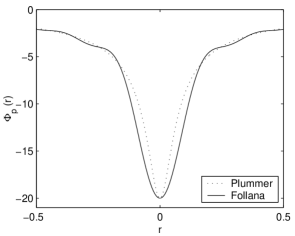
Figure 6: The Follona $(n=10)$ and the Plummer $(\varepsilon=0.05)$ potential in units of $Gm^{2}/R$, where $m$ is the particle mass.

Because the collapsed phase is probably sensitive to the short distance form of the potential we expect qualitatively a similar behavior only for the Plummer softened potential $(\xi=0)$ and a more different behavior for the potentials with short range repulsion $(\xi>1/3)$. Figure 7 shows the evolution of the inverse temperature as a function of the total energy $\varepsilon$ for two simulations with $\xi=0$ and $\xi=2/3$, respectively as well as the analytical curve calculated by Follana & Laliena. The figure confirms our expectations. We find for the Follana and the Plummer potential a negative specific heat in the same energy range. The system with a repulsive potential re-enters the zone of positive specific heat earlier than those without such a repulsion below the softening length. After entering the zone of negative specific heat a collapsing phase transition takes place, separating a high energy homogeneous phase from a collapsed phase. The collapsed phase resulting from the N-body simulations shows no core-halo structure. Such a structure is only formed due to relaxation after the cooling has stopped.

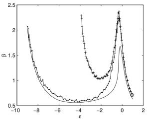
Figure 7: Inverse temperature $\beta$ versus energy $\varepsilon$ resulting from models with softened potentials. The solid line corresponds to the Follana potential. The other curves depict the evolution of the simulated systems. Crosses: Repulsive potential $(\xi=2/3)$. Dots: Plummer potential $(\xi=0)$. The circle indicates the initial states of the simulations.

6 Conclusions

For systems subjected to an energy flow we find:

• Potential perturbations caused by astrophysical objects passing in the vicinity of a self-gravitating system can compensate the energy loss due to dissipation, thus prevent the system from collapsing and maintain a statistical steady state.

• The statistical steady state is out of thermodynamic equilibrium and consists of a dense cold core moving in a hotter halo.

The results of the gravo-thermal experiments are:

• The range of negative specific heat agrees for a Plummer softening with the theory of self-gravitating systems with softened potentials.

• A softened potential incorporating short range repulsive forces reduces the range of negative specific heat. Systems with such repulsive forces re-enter the zone of positive heat capacity, thus becoming stable, at higher energies than those with “conventional” softening.