Estimate of the primordial magnetic field helicity

Abstract

Electroweak baryogenesis proceeds via changes in the non-Abelian Chern-Simons number. It is argued that these changes generate a primordial magnetic field with left-handed helicity. The helicity density of the primordial magnetic field today is then estimated to be given by $\sim 10^{2}n_{b}$ where $n_{b}\sim 10^{-6}$ /cm³ is the present cosmological baryon number density. With certain assumptions about the inverse cascade we find that the field strength at recombination is $\sim 10^{-13}$ G on a comoving coherence scale $\sim 0.1$ pc.

The helicity of a primordial magnetic field is of crucial importance in determining its subsequent evolution and in assessing whether the observed magnetic fields can be generated by amplification of the seed field by a galactic dynamo [1]. The average helicity density of a magnetic field, B, in a chosen volume $V$ is defined as:

$${\cal H}={1\over V}\int_{V}d^{3}x~{}{\bf A}\cdot{\bf B}$$ (1)

where ${\bf B}={\bf\nabla}\times{\bf A}$.

The connection between the helicity of primordial magnetic fields and baryon number is arrived at by considering the process of electroweak baryogenesis occurring at the time of the electroweak phase transition [2]. The genesis of baryons requires changes in the Chern-Simons number

$$CS={{N_{F}}\over{32\pi^{2}}}\int d^{3}x\epsilon_{ijk}\biggl{[}g^{2}\biggl{(}W^{a}_{ij}W^{ak} - {g\over 3}W^{ai}W^{bj}W^{ck}\biggr{)}$$ (2)

$$- {g^{\prime}}{}^{2}Y^{ij}Y^{k}\biggr{]}\ .$$ (3)

where, $N_{F}$ is the number of particle families, $W^{\mu a}$, $Y^{\mu}$ are the SU(2) and U(1) hypercharge gauge fields, $g$ and $g^{\prime}$ are SU(2) and U(1) gauge couplings, and $i,j,k=1,2,3$. Changes in $CS$ are achieved via the production and dissipation of non-perturbative field configurations such as the electroweak sphaleron [3], or linked loops of electroweak string[4, 5], or other equivalent configurations (for a review of electroweak strings see [6]). In the cosmological setting, it is believed that such configurations would be produced in the false vacuum phase due to the detailed dynamics of the electroweak phase transition, and would then decay in the true vacuum phase. Once they decay, the baryon number so produced cannot be washed out by the subsequent production and dissipation of more sphalerons or equivalent configurations.

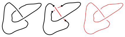
A feature of the baryon number producing intermediary field configurations is that they carry fluxes of non-Abelian magnetic fields that are twisted or linked. The simplest configuration to analyze is that of two linked electroweak strings (Fig. 1). Here the loops carry Z-magnetic flux and the Z magnetic lines are linked with each other.

Now consider the decay of the linked Z-string configuration. One path to decay is by the breaking of the loops of string. This occurs by the creation of monopole-antimonopole pairs. The segments of string then collapse. If the loops are very large, the whole process would be embedded in the highly conductive cosmological plasma in which the electromagnetic magnetic fields are frozen-in. Then the electromagnetic magnetic (B) field lines remain linked and the final helicity of the B field is related to that of the original Z-strings.

FIG. 1.: In the first figure, a pair of linked loops of Z-string are shown. They decay by the nucleation of monopole-antimonopole pairs (black circles in the middle figure) which get pulled apart by the strings. Magnetic field (B) lines (grey curves) run between the monopole and antimonopole. The whole system is embedded in a perfectly conducting plasma in which the B field lines are frozen-in. Finally the strings have decayed, leaving behind a B field configuration with helicity.

Other decay channels of the strings seem possible. For example, the loops could collapse before the strings break. In general we expect that the strings will collapse and decay into modes of B – since this is the only massless gauge field in the theory – and that these modes will retain some of the original helicity of the Z field. For an order of magnitude estimation of the helicity, it is sufficient to assume that the decay channel described above is not exceedingly improbable.

An electroweak sphaleron may also be interpreted as a segment of string terminating on a monopole and an antimonopole [4, 9, 10, 11]. The helicity is non-vanishing because the Z-string has a twist. The sphaleron is unstable to the untwisting of the monopole with respect to the antimonopole. This will transfer helicity from the twisted Z-string to the B field lines going from the monopole to the antimonopole as the sphaleron decays.

Having established a connection between the genesis of baryons and the helicity of magnetic fields, it is straight-forward to relate one to the other. The de-linking process shown in Fig. 1 leads to a change in the baryon number by $N_{F}\cos(2\theta_{w})$, where $\theta_{w}$ is the weak mixing angle (see [4, 5]), if the initial Z-string configuration has linkage $-1$. The B field flux of an electroweak monopole is $\Phi_{A}=(4\pi/e)\sin^{2}\theta_{w}$, where $e$ is the electromagnetic coupling (see [12, 6]). The helicity of the final configuration in Fig. 1 is $-2\Phi_{A}^{2}$. Hence, every baryon that is produced, causes a change in electromagnetic helicity

$$\Delta{H}=-2\left({{4\pi}\over e}\right)^{2}{{\sin^{4}(\theta_{w})}\over{N_{F}\cos(2\theta_{w})}}\sim-100$$ (4)

where we have used $\sin^{2}\theta_{w}=0.23$, $N_{F}=3$, and $e^{2}/4\pi\equiv\alpha=1/137$. Note that only changes in baryon number are related to changes in helicity. We further assume that the initial helicity density is negligible and this allows us to estimate the final helicity as $\Delta H$. (We are assuming that there are no sources besides electroweak baryogenesis for generating magnetic helicity in the very early universe.) The observed number density of baryons is $\sim 10^{-6}$/cm³ [13]. Therefore the average helicity of the primordial magnetic field is estimated to be $\sim-10^{-4}$/cm³ . In astrophysical units this is $\sim-(10^{-21}{\rm G})^{2}$-kpc. Note that this is not a root-mean-squared value for the magnetic helicity density but a mean local value. This is because our universe is observed to be made of matter and essentially no antimatter – supposedly due to the CP violation present in particle physics.

Once a helical magnetic field is produced there are a number of circumstances under which its helicity is conserved. In the MHD approximation, the magnetic field in Minkowski spacetime obeys the equation

$${{\partial{\bf B}}\over{\partial t}}={\bf\nabla}\times({\bf v}\times{\bf B})+{1\over{4\pi\sigma_{c}}}{\bf\nabla}^{2}{\bf B}$$ (5)

where ${\bf v}$ is the fluid velocity and $\sigma_{c}$ is the electrical conductivity of the plasma. First, if $\sigma_{c}$ is infinite, dissipation can be ignored and the evolution of the magnetic field only depends on the first term on the right-hand side of eq. (5). In this case, even the local helicity – defined by restricting $V$ in the integral in eq. (1) to volumes bounded by field lines [14] – is conserved. In a cosmological setting, the dissipation term can be ignored as compared to the effects of Hubble expansion on length scales above a certain critical scale called the “frozen-in” scale: $L_{f}\sim\sqrt{t/{4\pi\sigma_{c}}}$, where $t$ is the cosmic time. Magnetic fields that are coherent on scales larger than $L_{f}$ are said to be frozen-in and their helicity is conserved both locally and globally.

If the fluid velocities are small, it is possible that the first term on the right-hand side in eq. (5) can be ignored and only the dissipation term is relevant. In this case the field dies out exponentially fast and helicity is not conserved. However, if the fluid velocity is not negligible, the evolution of the field depends on both terms. In this situation, Taylor [14] has argued that the local helicity of the field changes due to reconnections of the field lines and hence is not conserved; however, the global helicity which is a sum over a lot of random local changes is still conserved. While there is no proof of Taylor’s conjecture, it leads to a successful explanation of the “reversed field pinch”. We shall assume that Taylor’s conjecture is true. The criterion for deciding if global helicity is conserved is that the magnetic Reynolds number ${\cal R}_{M}=4\pi\sigma_{c}Lv$ for magnetic fields on a length scale $L$ and characteristic fluid velocity $v$, should be large. With $\sigma_{c}\sim T/\alpha{\rm ln}(1/\alpha)\sim T/e^{2}$ [15, 16] and $L\sim 1/e^{2}T$, the length scale characteristic of gauge field configurations such as the sphaleron, the condition ${\cal R}_{M}>>1$ gives $v>>e^{4}/4\pi$. Whether this condition is met depends on the fluid dynamics during baryogenesis. Successful electroweak baryogenesis requires significant departures from thermal equilibrium which is likely to be accompanied by large fluid velocities. Therefore we will assume that the fluid velocities are large enough for ${\cal R}_{M}>>1$. As discussed above, under these circumstances, the field will evolve while conserving global magnetic helicity even though the field is not frozen-in.

The evolution of the field after production is a central problem in MHD. There are several features that are expected on theoretical grounds [14, 17, 18] and on the basis of numerical simulations [19, 20]. The first feature is that the magnetic field tangle is expected to evolve towards a configuration with ${\bf\nabla}\times{\bf B}=\beta{\bf B}$ for some constant $\beta$. Provided the field is characterized by a single length scale, this state is one of “maximal helicity” – a state in which the energy is minimum subject to the constraint of fixed global helicity. This expectation is supported by Taylor’s analysis of the reversed field pinch. The second feature is that helical magnetic fields are expected to “inverse cascade” – that is, energy will be transferred from small length scales to large length scales [21, 22, 17, 18, 19, 20] (though also see [23]). If $L(t)$ is the coherence scale of the field, the existing studies at large ${\cal R}_{M}$ in Minkowski spacetime find

$$L(t)=L_{*}\left({t\over{t_{*}}}\right)^{\xi}$$ (6)

where the exponent $\xi$ has been determined to be $1/2$ in numerical studies [19, 20], and $2/3$ in analytical studies under various approximations. The factor $L_{*}$ is the initial coherence scale of the magnetic field and $t_{*}$ is the time scale associated with the turbulence. We will take $t_{*}=L_{*}/v_{*}$ where $v_{*}$ is the typical fluid velocity. The third feature, as decribed earlier, is that the evolution is expected to conserve global helicity.

A little care is needed in applying eq. (6) to cosmology. The reason is that the origin of $t$ in eq. (6) is the time at the start of the simulation ($t=0$) while in cosmology the magnetic field is produced at the electroweak epoch. Furthermore, in cosmology, the flat (non-expanding) MHD equations can be used provided the time used is the conformal time [24, 25]. In a radiation dominated universe, the conformal time $\tau$ is related to the cosmic time $t$ by: $\tau=2t_{ew}^{1/2}(t^{1/2}-t_{ew}^{1/2})$. The factors of $t_{ew}$ have been chosen to give $\tau=0$ at $t=t_{ew}$ and $a(t_{ew})=1$ where $a(t)$ is the cosmological scale factor. Hence, in cosmology, the factor $(t/t_{*})^{\xi}$ in eq. (6) should be replaced by $(\tau/t_{*})^{\xi}$. It is more transparent and approximately equivalent to directly use eq. (6) for the first Hubble time – during which the expansion of the universe is irrelevant to the evolution of the magnetic field – and then use eq. (6) with $\xi$ replaced by $\xi/2$, together with a comoving factor, for further evolution in the radiation dominated epoch.

We can now evolve the magnetic field from the electroweak phase transition to the present epoch. We focus on the coherence scale of the field since the field strength can then be estimated quite easily using the conservation of helicity. At the electroweak scale we have seen that the magnetic Reynolds number is large and hence the coherence length will grow as in eq. (6) with $t_{*}=L_{*}/v_{*}$ and $L_{*}\sim 1/e^{2}T_{ew}$. We find that in one Hubble time,

$$L(t_{ew})\sim{1\over{T_{ew}}}(v_{*}t_{ew}T_{ew})^{\xi}\sim{1\over{T_{ew}}}\left({{T_{P}}\over{T_{ew}}}\right)^{\xi}$$

where $T_{P}=10^{19}$ GeV is the Planck energy and we have assumed fluid velocities: $v_{*}\sim 1$. For the slower estimate of the inverse cascade ($\xi=1/2$) this gives $L_{ew}\sim 10^{8}/T_{ew}\sim 10^{-8}t_{ew}$ which is greater than the frozen-in scale ($\sim 10^{7}/T_{ew}$). For the faster inverse cascade ($\xi=2/3$), the result is $L_{ew}\sim 10^{11}/T_{ew}$. Hence the magnetic field becomes coherent on a scale larger than the frozen-in scale within one Hubble expansion after production at the electroweak epoch. In this period we also expect the field to evolve towards maximal helicity with the dissipation of the non-helical component [26]. Once the field is maximally helical, further dissipation does not occur because such fields are force-free [18].

Further evolution of the magnetic field is a combination of Hubble expansion and inverse cascade. In a radiation dominated universe, this gives [18] $L(t)=L(t_{ew})({{T_{ew}}/T})^{1+\xi}$ We also check that the frozen-in scale $L_{f}$ grows as $(T_{ew}/T)^{3/2}$. Hence the coherence scale remains greater than the frozen-in scale for both values of $\xi$ and the helicity of the field continues to be conserved.

The next significant event occurs at the epoch of $e^{+}e^{-}$ annihilation at $T\sim 0.1$ MeV since the electrical conductivity of the plasma drops very suddenly. The electrical conductivity prior to the epoch is given by $\sigma_{c}\sim T/e^{2}$ [15, 16] while after this epoch it is given by $\sigma_{c}\sim 10^{-10}m_{e}/e^{2}$. This corresponds to a drop in conductivity by a factor of $10^{-9}$ and an increase of the frozen-in scale by $\sim 10^{4}$. The coherence scale just prior to $e^{+}e^{-}$ annihilation is:

$$L(t_{ee}-)=L_{f}(t_{ee}-){{L(t_{ew})}\over{L_{f}(t_{ew})}}\left({{T_{ew}}\over{T_{ee}}}\right)^{\xi-1/2}$$ (7)

where we have denoted quantities at $e^{+}e^{-}$ annihilation by the subscript $ee$ and $t_{ee}-$ denotes the time just prior to annihilation. Inserting numbers gives $L(t_{ee}-)=10L_{f}(t_{ee}-)$ for $\xi=1/2$ and $L(t_{ee}-)=10^{4}L_{f}(t_{ee}-)$ for $\xi=2/3$. Furthermore, at this stage the Reynolds number is ${\cal R}_{M}=4\pi\sigma_{c}Lv=(L/L_{f})^{2}>>1$ where we have made use of the definition of $L_{f}$ and have estimated the fluid velocity as due to cosmological expansion at the scale $L$: $v\sim L/t$. After $e^{+}e^{-}$ annihilation, however, $L/L_{f}\sim 10^{-3}$ if $\xi=1/2$ and $L/L_{f}\sim 1$ if $\xi=2/3$. In the first case, the magnetic Reynolds number is small and the fields are coherent on scales smaller than the frozen-in scale. Therefore with $\xi=1/2$ we expect the field to get dissipated. Only the Fourier modes of the magnetic field larger than the frozen-in scale can survive. In the second case, the magnetic Reynolds number may or may not be significantly larger than one and the coherence length of the field is comparable to the frozen-in scale. Therefore the coherence scale of the field will grow with the Hubble expansion and there may or may not be further inverse cascade. From now on we will only consider the value $\xi=2/3$ and give estimates of the coherence scale of the field both with and without inverse cascade in the post $e^{+}e^{-}$ annihilation universe.

The coherence scale at the recombination epoch can now be estimated as the scale at the electroweak epoch multiplied by the corresponding Hubble expansion factor and the inverse cascade factor:

$$L_{rec}=L_{ew}\left({{T_{ew}}\over{T_{eq}}}\right)^{1+\xi}\left({{T_{eq}}\over{T_{rec}}}\right)^{1+\xi/2}$$

where $L_{ew}\sim 10^{-5}$ cms, $\xi=0$ without inverse cascade and $\xi=2/3$ with inverse cascade, and the last factor takes into account the evolution in the matter-dominated era from the epoch of matter-radiation equality ($T_{eq}\sim 1$ eV) to the epoch of recombination ($T_{rec}\sim 0.1$ eV). This gives $L_{rec}\sim 10^{7}$ cms without inverse cascade and $L_{rec}\sim 10^{14}$ cms with inverse cascade.

The strength of the field can be estimated by using the conservation of helicity. At recombination the magnitude of helicity density is given by $\sim 10^{2}n_{b,rec}\sim 10^{5}$/cm³ or $\sim(10^{-13}{\rm G})^{2}$-($10^{14}$ cms). (The baryon density at recombination is $z_{rec}^{3}$ higher than that today where $z_{rec}\sim 10^{3}$ is the cosmological redshift at recombination.) So the maximally helical, primordial magnetic field with comoving coherence scale $\sim 0.1$ pc has a field strength $\sim 10^{-13}$ G at recombination.

The present scenario also allows us to estimate the net helicity of the galactic magnetic field. Both magnetic helicity and baryon number are conserved during galaxy formation when the protogalactic cloud collapses. During this collapse, the helicity and baryon densities increase due to the decrease in the cloud volume ($V$ in eq. (1)) but the ratio of the helicity density to the baryon density remains unchanged. Hence the helicity density of the galactic magnetic field can be estimated to be $\sim-10^{2}n_{b,gal}\sim-10$/cm³ which is $\sim-(10^{-19}{\rm G})^{2}$-kpc. Subsequent evolution of the magnetic field during galaxy formation, including the amplification by a turbulent dynamo, does not significantly change the global helicity [27] and we expect this estimate to hold even today. Furthermore, we have earlier noted that the magnetic helicity density has the same sign everywhere and is negative. Hence the magnetic field in all the different galaxies should be left-handed. The left-handedness of the magnetic field could also lead to a CP violating signature in the cosmic microwave background radiation [28].