Morphological fluctuations of large–scale structure:
the PSCz survey

In a follow–up study to a previous analysis of the IRAS 1.2Jy catalogue, we quantify the morphological fluctuations in the PSCz survey. We use a variety of measures, among them the family of scalar Minkowski functionals. We confirm the existence of significant fluctuations that are discernible in volume–limited samples out to 200$h^{-1}$Mpc. In contrast to earlier findings, comparisons with cosmological $N$–body simulations reveal that the observed fluctuations roughly agree with the cosmic variance found in corresponding mock samples. While two–point measures, e.g. the variance of count–in–cells, fluctuate only mildly, the fluctuations in the morphology on large scales indicate the presence of coherent structures that are at least as large as the sample.

1 Introduction

Nowadays, one of the primary goals of cosmology is the verification of the plethora of models that have emerged over the years. To that end, experiments are being conducted and planned that will ultimately yield deep and wide galaxy surveys and high–resolution maps of the Cosmic Microwave Background. In parallel to the preparation of these large datasets, statistical methods that are both easy to interpret and efficient to implement are being developed.

A few years ago, the Minkowski functionals (MFs) were introduced into cosmology by Mecke et al. (1994). The MFs can be calculated from contemporary datasets rather efficiently, and consequently numerous applications (see Kerscher 2000 and references therein, vector–valued MFs are described in Beisbart et al. 2001) have established the MFs as a suitable tool for quantifying the morphological properties of the large–scale structure in the Universe . Apart from their practical advantages, MFs provide a mathematically well–founded systematic framework for the study of statistical morphology and contain other higher–order statistics that were employed previously.

The present work extends the scope of an earlier paper on the morphological fluctuations in the IRAS 1.2Jy catalogue of infrared galaxies (Kerscher et al. 1998), by using its much deeper successor, the recently compiled PSCz survey (Saunders et al. 2000). However, we do not simply repeat the previous study with the enlarged dataset, but devise additional sensible tests in order to assess the quality of the data and to compare the observational data to $N$–body simulations. Kerscher et al. (1998) detected, quite unexpectedly at that time, significant fluctuations in the morphological properties between the northern and southern hemispheres of the IRAS 1.2Jy catalogue in volume–limited samples of up to 200$h^{-1}$Mpc depth. While these findings were shown to be significant and not due to deficiencies of the data, simulations could not reproduce them, even though they were specifically designed for that purpose. Meanwhile, simulations have improved, mainly with respect to the size of the simulation box. We shall demonstrate that the large fluctuations seen in the IRAS 1.2Jy catalogue can still be found in the PSCz survey. However, state–of–the–art simulations of Cold Dark Matter (CDM) scenarios are now capable of predicting sufficient cosmic variance. Another analysis of the PSCz sample with Minkowski functionals by Basilakos et al. (2001) focused on the shape of super–clusters.

This article is organised as follows: Sect. 2 briefly explains how Minkowski functionals are calculated from the PSCz dataset and summarises our findings in a qualitative way. It also contains a discussion of possible systematic effects and results obtained with other statistical methods. Sect. 3 compares the observational data with an analytical model and a set of mock catalogues. We summarise and provide an outlook in Sect. 4. Finally, a few necessary mathematical results are given in the Appendix.

2 Measuring the morphology of the PSCz survey

2.1 Minkowski functionals

Table 1: Minkowski functionals in three–dimensional space expressed in terms of more familiar geometric quantities.

	geometric quantity	$\mu$	$M_{\mu}$	$M_{\mu}(B_{r})$
$V$	volume	0	$V$	$4\pi r^{3}/3$
$A$	surface area	1	$A/8$	$\pi r^{2}/2$
$H$	mean curvature	2	$H/(2\pi^{2})$	$2r/\pi$
$\chi$	Euler characteristic	3	$3\chi/(4\pi)$	$3/(4\pi)$

In order to quantify the morphology within the PSCz survey (Saunders et al. 2000) with Minkowski functionals, we interpret the redshift space positions $\{{\mathbf{x}}_{i}\}_{i=1}^{N}$ of the $N$ galaxies in the sample as a realisation of a stationary point process. Adopting the Boolean grain method of Mecke et al. (1994), we decorate each point ${\mathbf{x}}_{i}$ with a sphere $B_{r}({\mathbf{x}}_{i})$ of radius $r$ and consider the union set ${\cal A}_{r}=\bigcup_{i=0}^{N}B_{r}({\mathbf{x}}_{i})$. Hadwiger (1957) has shown that in three–dimensional space the four Minkowski functionals $M_{\mu}({\cal A}_{r})$, with $\mu=0,1,2,3$ provide a complete morphological characterisation of the body ${\cal A}_{r}$. Table 1 summarises the interpretations of these functionals in terms of well–known geometrical and topological quantities.

Reduced, dimensionless Minkowski functionals $\Phi_{\mu}({\cal A}_{r})$ can be constructed by normalising with the Minkowski functionals $M_{\mu}(B_{r})$ of a single sphere,

$$\Phi_{\mu}({\cal A}_{r})=\frac{M_{\mu}({\cal A}_{r})}{NM_{\mu}(B_{r})}.$$ (1)

The mean number density $\rho$ can be estimated in a sample by $N/|\Omega|$, where $|\Omega|$ is the volume of the sample. For a Poisson process these functionals can be calculated analytically (Mecke and Wagner 1991) as functions of $\eta=M_{0}(B_{r})\rho$, the expected number of galaxies in a sphere of radius $r$:

$$\begin{array}[]{rl}\Phi_{0}^{\rm P}&=\left(1-{\rm e}^{-\eta}\right)\ \eta^{-1},\\ \Phi_{1}^{\rm P}&={\rm e}^{-\eta},\\ \Phi_{2}^{\rm P}&={\rm e}^{-\eta}\ (1-\frac{3\pi^{2}}{32}\eta),\\ \Phi_{3}^{\rm P}&={\rm e}^{-\eta}\ (1-3\eta+\frac{3\pi^{2}}{32}\eta^{2}).\end{array}$$ (2)

Obviously, the Minkowski functionals $\Phi_{\mu}^{\rm P}({\cal A}_{r})$, $\mu=1,2,3$, contain a damping factor ${\rm e}^{-\eta}$. A similar exponential decay is also found for more general cluster processes. To facilitate the comparison between the data and different models on large scales, we reduce the functionals by this factor and consider the quantities

$$\phi_{\mu}({\cal A}_{r})\equiv\frac{\Phi_{\mu}\left({\cal A}_{r}\right)}{\Phi_{1}^{\rm P}(r)}$$ (3)

throughout the following analysis.
Effective methods to calculate the Minkowski functionals for empirical data points are described in Mecke et al. (1994). To correct for boundary effects without applying unnecessary statistical assumptions we proceed as Schmalzing et al. (1996) (see also Mecke and Wagner 1991; Kerscher et al. 1997).

2.2 Selection of the samples

A detailed description of the PSCz galaxy catalogue may be found in Saunders et al. (2000). For our analysis we extract volume–limited samples (Table 2) from the PSCz survey within the standard masked area. The velocities of the galaxies in the local group frame ($v=v_{\rm hel}+\sin(l)\cos(b)\ 300{\rm km/s}$) are converted into luminosity distances assuming $q_{0}=0.5$ and $\Lambda=0$.

Table 2: Volume–limited samples from the PSCz survey. $N$ denotes the number of galaxies.

depth [$h^{-1}$Mpc]	flux limit [Jy]	$N_{\rm north}$	$N_{\rm south}$
100	0.6	1119	1078
100	0.8	676	661
100	1.2	311	332
200	0.8	337	323

In order to simplify the boundary corrections, we approximate the sample geometry by a spherical cap with galactic latitude $b\geq 5^{\circ}$ for the northern sample and with $b\leq-5^{\circ}$ for the southern part. Since by doing so, we neglect some regions which were excluded due to galactic absorption or confusion in the IRAS PSC maps, we filled these empty regions with random points with the same number density as in the fully sampled region. Differences in the Minkowski functionals between the filled and unfilled samples are barely visible.

Another issue to be discussed is the flux limit of the PSCz survey. Tentatively, we evaluated the Minkowski functionals for a series of volume–limited samples with 100$h^{-1}$Mpc depth , but with varying limiting flux. Only for limiting fluxes above 0.8Jy the Minkowski functionals stabilise. Likewise, Tadros et al. (1999) find stable results only for a flux limit larger than 0.75Jy. Therefore, we shall adopt a flux limit 0.8Jy for all of our analyses.

This kind of flux dependence does not show up in two–point measures. The two–point correlation function $\xi_{2}$, e.g., does not change significantly when the flux cut is varied. Even the mark correlation functions (Beisbart and Kerscher 2000; Szapudi et al. 2000) do not show any luminosity–dependent clustering at the two–point level. Further tests on selection effects will be discussed in Sect. 2.4.

2.3 Fluctuating morphology

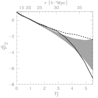
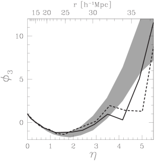
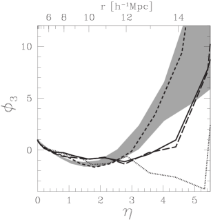
Fig. 1 displays the values of the reduced Minkowski functionals $\phi_{\mu}$ as functions of the $\eta$ for the southern and northern parts of the PSCz survey at a limiting depth of $100{{h^{-1}{\rm Mpc}}}$. For comparison, we also show the expectation values for a Poisson process with the same number density.

In both parts of the sample the galaxy clustering is noticeably stronger than in the case of randomly distributed points. Moreover, the northern and southern parts differ significantly in their morphological features, the northern part being less lumpy. The most conspicuous features are the enhanced surface area $\phi_{1}$ in the southern part on scales larger than 10$h^{-1}$Mpc, and the decrease of the Euler characteristic $\phi_{3}$, which sets in at 12$h^{-1}$Mpc. On scales above 10$h^{-1}$Mpc, the integrated mean curvature $\phi_{2}$ and the Euler characteristic $\phi_{3}$ are negative, indicating an interconnected system of tunnels. In the southern part $\phi_{3}$ remains negative out to large scales, and the large–scale structure is dominated by interconnected tunnels contrary to the northern part, where completely enclosed voids yield positive contributions to the Euler characteristic.

Figure 1: The MFs of volume–limited samples from the PSCz survey with 100$h^{-1}$Mpc depth. The southern (solid) and northern parts (dashed) are plotted separately, and for comparison the one–sigma fluctuations (shaded regions) for a Poisson process with the same number density are also shown.

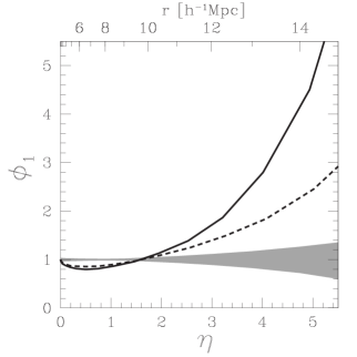
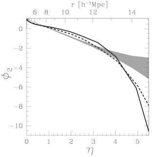
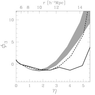
The morphological fluctuations observed in the PSCz survey appear comparable to those found in the IRAS 1.2Jy catalogue (Fisher et al. 1995; Kerscher et al. 1998). To verify this, we extract volume–limited samples from the PSCz survey with a limiting flux of 1.2Jy. For this comparison we use the Euclidean redshift space distance as in our original analysis of the IRAS 1.2Jy catalogue. In the southern part, we find no difference in the Minkowski functionals. The northern part of this PSCz sample, however, contains less galaxies than the corresponding IRAS 1.2Jy subsample, probably due to the more restrictive selection criteria imposed on the PSCz survey. But still, the MFs of the randomly sub–sampled northern part of the IRAS 1.2Jy nearly overlap with the PSCz sample. Hence we are confident that the MFs pick up the underlying large–scale structure, which should of course be the same in both catalogues.

2.4 Selection effects and deeper samples

To strengthen our claims regarding the morphological fluctuations, we have to exclude some possible sources of error. To begin with, an analysis of the 100$h^{-1}$Mpc sample with a more conservative cut at $|b|\geq 10^{\circ}$ instead of $5^{\circ}$ leads to nearly identical results for the Minkowski functionals.

To check whether our results are influenced by some peculiar alignment of points, we considered a subsample with only 90% of the galaxies randomly chosen from the volume–limited sample. Repeating this jackknife procedure, we calculate the mean and the error of the Minkowski functionals. Still the same prominent fluctuations between north and south can be seen. These errors are smaller than the fluctuations in the random point set. We want to emphasise that this jackknife error can only serve as an internal consistency check; it does not give a reliable estimate of the fluctuations in the underlying galaxy distribution (Snethlage 1999).

Moreover, we select subsamples with “warm” and “cold” galaxies as determined from the flux ratio $\frac{f_{100}}{f_{60}}\leq 2$ and $\frac{f_{100}}{f_{60}}>2$, respectively, with $f_{100}$ the flux at 100$\mu$m and $f_{60}$ the flux at 60$\mu$m. In both samples we find fluctuations between north and south, comparable to those in the combined sample. Finally, the strength of the fluctuations hardly diminishes if we consider the measured velocities without a heliocentric correction.

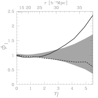
To see whether these fluctuations persist on even larger scales, we investigate volume–limited samples with 200$h^{-1}$Mpc depth (Fig. 2). On small scales, both in the northern and the southern part, the MFs indicate clustering. Again and in particular on large scales, the MFs of the southern part differ from the MFs of the northern part, showing approximately the same pattern as in the volume–limited sample with 100$h^{-1}$Mpc. The fluctuations are now only slightly larger than the one–sigma fluctuations observed in a Poisson process with the same number density. As already demonstrated by Kerscher et al. (1998), the morphology of such a sparsely sampled catalogue tends to resemble a pure random sample as dilution increases (see also Sect. 2.6). The Minkowski functionals in the volume–limited samples with 150$h^{-1}$Mpc  depth give comparable results, showing fluctuations of a strength between the fluctuations of the 100$h^{-1}$Mpc and the 200$h^{-1}$Mpc sample.

Figure 2: The Minkowski functionals of volume–limited samples with 200$h^{-1}$Mpc depth. See Fig. 1 for an explanation of plotting styles.

In Kerscher et al. (1996) we could show that the morphological discrepancies in the 1.2Jy galaxy catalogue are not a special north–south anisotropy. We proceed similar by cutting both the northern and the southern part along the $yz$–plane (in galactic coordinates) into two pieces with the same volume. The Minkowski functionals of the four samples are shown in Fig. 3 confirming that the fluctuations are not a peculiar north–south anisotropy, but actually reflect the generic cosmic variance.

Figure 3: The MFs of volume–limited samples with 100$h^{-1}$Mpc depth from the PSCz survey. Four different parts of the sample are considered separately: southern left (solid), southern right (dotted), northern left (short dash), northern right (long dashed). As before, the area shows a Poisson process.

2.5 Other measures

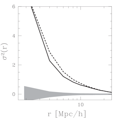
Both from a physical and a methodological point of view, it is interesting to compare the performance of the MFs with other statistics. For instance, the well–known $\sigma^{2}(r)$ measures the fluctuations of the number of galaxies in a sphere with radius $r$ in excess of a Poisson process. $\sigma^{2}(r)$ is a pure second–order measure. To calculate $\sigma^{2}(r)$ for the PSCz samples, we estimate the correlation integral $C(r)$, the mean number of points in a sphere with radius $r$ centred on one galaxy, and use the relation

$$\sigma^{2}(r)=\frac{C(r)}{\rho\ 4\pi/3\ r^{3}}-1.$$ (4)

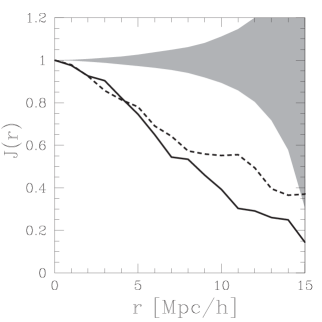
Our results do not depend on the estimator for $C(r)$ (Kerscher 1999). Fig. 4 illustrates that on the two–point level there are no significant fluctuations between north and south.

Hence, the fluctuations observed with the MFs are a genuine effect of higher–order correlations, illustrating that low–order statistics such as the number density or the two–point correlation function may miss global features of the large–scale structure. Such higher–order correlations may originate from coherent elements like filaments or walls with an extent comparable to or larger than the size of the sample, in our case 100$h^{-1}$Mpc. This conjecture is also supported by visual inspection of the large–scale structure (see e.g. Huchra et al. 1990).

Figure 4: Fluctuation of count–in–cells $\sigma^{2}(r)$ of the volume–limited sample with 100$h^{-1}$Mpc depth from the PSCz survey. Plotting styles are the same as in Fig. 1.

Other methods to characterise the spatial distribution of points are

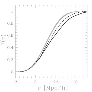
• the spherical contact distribution $F(r)$, i.e. the distribution function of the distances $r$ of galaxies from an arbitrary point in space,

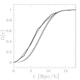
• the nearest neighbour distance distribution $G(r)$ defined as the distribution function of distance $r$ of a galaxy to the nearest other galaxy,

• and the ratio suggested by van Lieshout and Baddeley (1996)

  $$J(r)=\frac{1-G(r)}{1-F(r)}.$$ (5)

For a Poisson distribution one finds

$$G(r)=F(r)=1-\exp\left(-\rho\frac{4\pi}{3}r^{3}\right)$$ (6)

and consequently $J(r)=1$. We use the minus–estimators, as discussed by Kerscher et al. (1998), to determine $F$ and $G$ from the galaxy distribution. The spherical contact distribution equals the volume density of the first Minkowski functional and one minus the void probability: $F(r)=M_{0}({\cal A}_{r})/|\Omega|=1-P_{0}(B_{r})$.

In Fig. 5 we show the results for the spherical contact distribution $F(r)$, the nearest neighbour distribution $G(r)$, and the $J(r)$ function. The fluctuations within the PSCz survey in comparison to a Poisson process are most prominent in the spherical contact distribution $F(r)$, and slightly less pronounced in the $J(r)$–function. Virtually no fluctuations are detected with the nearest neighbour distance distribution $G(r)$. The reason is that $G(r)$ focuses on the small–scale features, which do not fluctuate strongly on the scales probed by the PSCz survey, while $F(r)$ and $J(r)$ are capable of tracing the large–scale geometry and topology of the galaxy distribution.

Figure 5: The panels show the $F(r)$, $G(r)$, and $J(r)$ function of volume–limited samples from the PSCz survey with 100$h^{-1}$Mpc depth. Plotting styles are the same as in Fig. 1.

2.6 From small to large scales

In the preceding sections we saw that the morphology on small scales up to $10{{h^{-1}{\rm Mpc}}}$ does not show the strong fluctuations we observed on larger scales. To understand this behaviour in more detail we expand the Minkowski functionals $\Phi_{\mu}({\cal A}_{r})$ as a series in $\eta=M_{0}(B_{r})\rho$ around zero. Based on the expansion in terms of $n$–point densities (Mecke et al. 1994, Eq. (25)) we obtain

$$\phi_{\mu}({\cal A}_{r})=1-\\ \eta\frac{3}{2r^{3}}\int_{0}^{2r}{\rm d}ss^{2}\tfrac{M_{\mu}(B_{r}(0)\cap B_{r}(s))}{M_{\mu}(B_{r})}\left[1+\xi_{2}(s)\right]+{\cal O}(\eta^{2})\;.$$ (7)

The integral together with the ratio in front yields a dimensionless geometric factor depending on the correlation function $\xi_{2}(s)$. The higher–order terms proportional to $\eta^{n-1}$ include integrals with intersections of $n$ spheres weighted by the $n$–point densities. For small $\eta$ only the two–point correlation function is important, but the MFs become increasingly more sensitive to higher–order correlations with larger $\eta$. A small $\eta$ may be obtained either from a low number density $\rho$ or a small radius $r$ of the spheres.

The two–point correlation function of the PSCz survey shows only tiny fluctuations between north and south as can be deduced from Fig. 4. On small scales with $\eta\ll 1$ the numerical values of the Minkowski functionals may be reproduced using Eq. (7) with the observed two–point correlation function and mean density. This explains why for small radii the morphological fluctuations are negligible. The expression (7) also explains why the MFs of dilute samples tend to look more like those of a Poisson process.

3 Comparing data and models

3.1 Second-order moments of Minkowski functionals

To compare the fluctuations of the observed Minkowski functionals with different models we will use the dimensionless second–order moments (see also Eq. (11))

$$m_{\mu\mu}(\eta)=\frac{M_{0}(B_{r})}{M_{\mu}(B_{r})^{2}|\Omega|}\left\langle\Big{(}M_{\mu}({\cal A}_{r})-\langle M_{\mu}({\cal A}_{r})\rangle\Big{)}^{2}\right\rangle,$$ (8)

where $|\Omega|$ is the sample volume. The $m_{\mu\mu}$ are estimated either on the base of samples from simulations or from the real data using the standard estimator for a variance.

$$m_{\mu\mu}(\eta)=\frac{M_{0}(B_{r})}{M_{\mu}(B_{r})^{2}|\Omega|}\ \frac{1}{N_{s}-1}\sum_{i=1}^{N_{s}}\Big{(}M_{\mu}^{(i)}-M_{\mu}\Big{)}^{2},$$ (9)

where $N_{s}$ is the number of samples, $M_{\mu}=\frac{1}{N_{s}}\sum_{i=1}^{N_{s}}M_{\mu}^{(i)}$ is the sample mean, and the $M_{\mu}^{(i)}$ are the MFs of the $i$th sample. From the PSCz catalogue we take two samples, the southern and the northern part with a depth of 100$h^{-1}$Mpc each.

In Appendix A the fluctuations for a Poisson and a binomial process are given analytically. The comparison with the estimated fluctuations from the PSCz survey in Fig. 6 indicates that the observed dimensionless fluctuations are significantly larger than the $m_{\mu\mu}^{\text{P}}$ for a Poisson process with the same number density. Qualitatively, the fluctuations from the PSCz survey show similar features as for a Poisson process, i.e. the functional form and the relative strengths of the fluctuations are comparable. Only the surface area is qualitatively different on large scales. Of course, an estimate of fluctuations from two samples only should be considered as a first rough estimate. Also the zero variance determined from the PSCz for some radii is an artifact of using only two samples.

Figure 6: The dimensionless fluctuations of the Minkowski functionals for a Poisson process are shown in the left plot. In the middle plot the estimated variances $m_{\mu\mu}$ from the volume–limited sample of the PSCZ with 100$h^{-1}$Mpc depth, and in the right plot the estimated variances from the $\Lambda$CDM mock samples are shown (notice the different scaling). The $\tau$CDM mock samples show similar fluctuations.

3.2 Comparison with CDM simulations

More realistic models to compare our data to are based on $N$–body simulations. We use mock galaxy catalogues constructed from the VIRGO consortium’s Hubble volume simulations. The mock catalogues were kindly provided to us by Shaun Cole. From these mock catalogues we extract volume–limited samples with a depth of 100$h^{-1}$Mpc similar to the observed galaxy samples. The CDM $N$–body simulations were performed by the VIRGO consortium and comprise a $\Lambda$CDM ($\Omega_{m}=0.3$, $\Omega_{\Lambda}=0.7$, $\sigma_{8}=0.9$) and a $\tau$CDM ($\Omega_{m}=1$, $\Omega_{\Lambda}=0$, $\sigma_{8}=0.6$) simulation, conducted in a box with a side length of $3h^{-1}$Gpc and $2h^{-1}$Gpc, respectively (for details see Evrard et al. 2001 and their web–site). Mock catalogues were generated with methods similar to those used by Cole et al. (1998): the galaxies were extracted from the distribution of the dark matter particles employing a biasing scheme; luminosities have been assigned according to the observed luminosity function (for details see Cole et al. 1998 and their web–site). The observer position was not chosen at random but selected to satisfy criteria similar to those of the local group, with respect to the local density, the CMB dipole, and the local shear (Baugh et al. 2001). We used the first eleven mock catalogues constructed from each simulation.

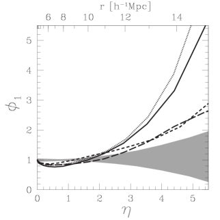
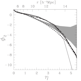
The Minkowski functionals for the mock samples were calculated in redshift space within the same sample geometry as for the PSCz survey. Considering north and south separately we can use $N_{s}=22$ samples per simulation to estimate the mean MFs and their variance. In Fig. 7 the mean MFs of the mock samples are compared with the mean MFs of the PSCz catalogue. Within the estimated errors, the large scale morphology of the galaxy distribution is marginally reproduced by the $\Lambda$CDM model, whereas the $\tau$CDM model is too lumpy.

Figure 7: In addition to the mean MFs from the PSCz survey (solid), this plot displays the mean results from the mock sample constructed from the $\Lambda$CDM (dotted) and $\tau$CDM (dashed) simulation. The shaded area marks the one–sigma region determined from the $\Lambda$CDM simulation. The $\tau$CDM simulation shows similar fluctuations.

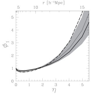
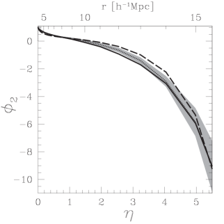
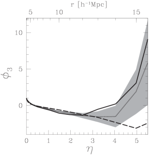
The main issue is whether these mock catalogues are able to reproduce the large morphological fluctuations in the PSCz survey. This is of specific interest since it turned out that a simulation, designed to match the local distribution of IRAS galaxies, was not able to reproduce the fluctuations in the 1.2Jy galaxy survey (Kerscher et al. 1998). Similar large–scale fluctuations as observed in the galaxy distribution may indeed be found in the mock catalogues of both models (see Fig. 6). At least, the amplitude of the fluctuations $\widehat{m}_{\mu\mu}$ determined from real data and the mock samples are of the same order of magnitude. The fluctuations in the number density between of the volume–limited samples extracted from the mock catalogues are in full agreement with the $\sigma^{2}$ expected for the models at the sample size, but are larger than the number density fluctuations between the northern and southern PSCz samples. These fluctuations in the number density seem to cause the increased fluctuations in $\widehat{m}_{00}$ for the mock samples.

4 Summary

We investigate the morphology of the galaxy distribution in the PSCz survey. In order to quantify the geometrical and topological features, we use the fluctuations of count–in–cells as a two–point measure, as well as a number of higher–order statistics, namely the nearest neighbour distance distribution function, the void probability, the $J$–function, and the family of scalar Minkowski functionals. We find appreciable fluctuations between the northern and southern parts of the survey, confirming earlier findings from the IRAS 1.2Jy catalogue (Kerscher et al. 1998). These fluctuations are discernible in volume–limited samples of as much as 200$h^{-1}$Mpc depth. By inspecting subsamples we show that these fluctuations are not due to a specific north–south anisotropy, but are an intrinsic feature of the galaxy distribution on large scales.

The comparison with the fluctuations in mock–catalogues shows that $N$–body simulations of two CDM models in boxes with a side length of $2$ and $3h^{-1}$Gpc followed by a suitable biasing procedure are able to account for the observed morphological fluctuations in the galaxy distribution. This was not the case when we compared the fluctuations in the IRAS 1.2Jy with those determined from a simulation in a smaller box with 250$h^{-1}$Mpc side length. Concerning the mean values of the Minkowski functionals, the $\tau$CDM simulation is not able to explain the observed large–scale morphology. Marginally, the $\Lambda$CDM model succeeds.

Speaking of fluctuations, one usually thinks of the fluctuations in the number of galaxies, the fluctuations of count–in–cells $\sigma^{2}$, or the power spectrum quantifying the amount of fluctuations in a Fourier mode of the density contrast. Both measures quantify the galaxy distribution at the two–point level, and are therefore unable to detect coherent large–scale structure elements like walls and filaments (see e.g. Szalay 1997; Schmalzing et al. 1999; Chiang and Coles 2000). Indeed, our investigations of the galaxy distribution in the PSCz survey using $\sigma^{2}$ show no significant fluctuations at the two–point level between the northern and southern parts of the galaxy sample.

Minkowski functionals, however, incorporate correlations of arbitrary order and quantify the connectivity of large–scale structure elements in the galaxy distribution. The amplitude of the morphological fluctuations in samples with an extent of 100$h^{-1}$Mpc is approximately three times larger than expected for a Poisson process. The morphological fluctuations remain detectable even in a 200$h^{-1}$Mpc sample, but since the deeper volume–limited samples are sparser and therefore more similar to a Poisson process, the results become less significant. The structural differences between the northern and southern parts of the PSCz sample show up prominently in the Minkowski functionals for radii above 10$h^{-1}$Mpc. As already mentioned, the number density and also the two–point correlations show only small fluctuations. This indicates that a variety of coherent structures with a low density contrast and an extent of more than 100$h^{-1}$Mpc, perhaps 200$h^{-1}$Mpc, are shaping the large–scale structure of the Universe. In this sense, our analysis quantifies the visual impression of features like the great wall in the CfA2 catalogue (Huchra et al. 1990).

Structures like walls and filaments were predicted by analytical and numerical work based on the Zel’dovich approximation (Arnol’d et al. 1982; Doroshkevich et al. 1996) and related approximations (Kofman et al. 1992; Bond et al. 1996). They are generic features of the gravitational collapse for CDM–like initial conditions, as numerous $N$–body simulations could verify (Melott and Shandarin 1990; Jenkins et al. 1998). To detect these morphological features, especially if they show up only at a low density contrast, sensitive methods like the Minkowski functionals are needed. They allow us to quantify the geometry and topology of the network of walls, filaments, and voids seen in the distribution of galaxies.

Appendix A Fluctuations of the Minkowski functionals for a Poisson model

The simplest point process, and thus the simplest reference model to compare real data to, is a stationary Poisson point process lacking any spatial correlations. In this appendix we give the exact expressions for the variances of the Minkowski functionals for a Poisson process and a binomial process. These results prove useful both to estimate the fluctuations of the morphological properties for finite samples, and to serve as a reference model for a comparison with fluctuations in empirical datasets (Fig. 6). Here we only explain the basic notions and list the results for three dimensions. A full derivation of the variances for the Minkowski functionals as well as their covariances in any dimension can be found in (Mecke 2001).

Let us first consider a stationary Poisson point process with number density $\rho$ in a sample $\Omega$ of volume $|\Omega|$ embedded into three–dimensional Euclidean space. We are interested in the morphological fluctuations as quantified by the covariances of the Minkowski functionals $M_{\mu}({\cal A}_{r})$ for the Boolean grain model. For convenience, we divide the variances by the Minkowski functionals $M_{\mu}(B_{r})$ of a single sphere $B_{r}$ of radius $r$ and express them as functions of $\eta\equiv M_{0}(B_{r})\rho$ such that all quantities are dimensionless and may be compared quantitatively:

$$m_{\mu_{1}\mu_{2}}(\eta)\equiv\frac{M_{0}(B_{r})}{|\Omega|M_{\mu_{1}}(B_{r})M_{\mu_{2}}(B_{r})}\Bigg{\langle}\Big{(}M_{\mu_{1}}({\cal A}_{r})-\big{\langle}M_{\mu_{1}}({\cal A}_{r})\big{\rangle}\Big{)}\Big{(}M_{\mu_{2}}({\cal A}_{r})-\big{\langle}M_{\mu_{2}}({\cal A}_{r})\big{\rangle}\Big{)}\Bigg{\rangle},$$ (10)

where $\langle\cdot\rangle$ denotes the average over the statistical ensemble.

The Minkowski functionals $M_{\mu}({\cal A}_{r})$ of a union set of balls can be represented either as an integral over the volume of the set ($\mu=0$) or as integrals over the $(d-\lambda)$–dimensional intersections of $\lambda$ spherical boundaries for $\mu=1,\ldots,d$ and $\lambda=1,\ldots,\mu$; in the latter case local curvatures arise as weightings. Therefore, the variances $m_{\mu_{1}\mu_{2}}$ can be decomposed into a series of curvature–weighted structure functions $M_{\mu_{1}\mu_{2}}^{\lambda_{1}\lambda_{2}}(\eta,s)$ containing the contributions of the $(d-\lambda_{i})$–dimensional spherical intersections to $M_{\mu_{i}}$ for $i=1,2$ (Mecke 2001):

$$m_{\mu_{1}\mu_{2}}(\eta)=\sum_{\lambda_{1}=0}^{\mu_{1}}\sum_{\lambda_{2}=0}^{\mu_{2}}\int\limits_{0}^{1}{\rm d}s\ M_{\mu_{1}\mu_{2}}^{\lambda_{1}\lambda_{2}}(\eta;s).$$ (11)

For the following listing of the structure functions $V$ denotes the volume of the sphere $B_{r}$, and $V(s)$ is the normalized volume of two overlapping spheres $B_{r}({\mathbf{x}}_{1})$ and $B_{r}({\mathbf{x}}_{2})$ of radius $r$ and centre ${\mathbf{x}}_{i}$ given by

$$V(s)=\frac{V(B_{r}({\mathbf{x}}_{1})\cup B_{r}({\mathbf{x}}_{2}))}{V(B_{r})}=1+\frac{3}{2}s-\frac{1}{2}s^{3},$$ (12)

where $s=\frac{\left|{\mathbf{x}}_{2}-{\mathbf{x}}_{1}\right|}{2r}$ denotes the normalized distance of the spheres. Note, that the structure functions are symmetric, $M^{\lambda_{1}\lambda_{2}}_{\mu_{1}\mu_{2}}(\eta,s)=M^{\lambda_{2}\lambda_{1}}_{\mu_{2}\mu_{1}}(\eta,s)$, and vanish, if $\lambda_{i}>\mu_{i}$ for $i=1$ or $i=2$. We get

$$M_{00}^{00}(\eta;s)=24s^{2}\left({\rm e}^{-\eta V(s)}-{\rm e}^{-2\eta}\right),$$ (13)

$$M_{\mu 0}^{\lambda 0}(\eta;s)=(-1)^{\lambda+1}\frac{\eta^{\lambda}}{\lambda!}\left(\bar{M}^{\lambda}_{\mu}{\rm e}^{-2\eta}-\check{M}^{\lambda}_{\mu}{\rm e}^{-\eta V(s)}\right),$$

$$M_{\mu_{1}\mu_{2}}^{\lambda_{1}\lambda_{2}}(\eta;s)=(-1)^{\lambda_{1}+\lambda_{2}}{\rm e}^{-\eta V(s)}\sum\limits_{l=0}^{\lambda_{2}}\frac{\eta^{\lambda_{1}+\lambda_{2}-l}}{l!(\lambda_{1}-l)!(\lambda_{2}-l)!}M^{\lambda_{1}\lambda_{2}}_{\mu_{1}\mu_{2};l}-24s^{2}\;M_{\mu_{1}}^{\lambda_{1}}M_{\mu_{2}}^{\lambda_{2}}.$$

The structure amplitudes $\bar{M}_{\mu}^{\lambda}$, $M_{\mu}^{\lambda}(\eta)$, $\check{M}^{\lambda}_{\mu}(s)$ and $M^{\lambda_{1}\lambda_{2}}_{\mu_{1}\mu_{2};l}(s)$ arising in these formulae vanish if $\lambda>\mu$ and $\lambda_{i}>\mu_{i}$ for $i=1$ or $i=2$, respectively. For the other cases one finds the following: the quantities $\bar{M}^{\lambda}_{\mu}$, with

$$\begin{split}\bar{M}^{1}_{\mu}&=1,\\ \bar{M}^{2}_{2}&=\frac{2M_{1}(B_{r})^{2}}{M_{0}(B_{r})M_{2}(B_{r})}=\frac{3\pi^{2}}{16},\\ \bar{M}^{2}_{3}&=\frac{6M_{1}(B_{r})M_{2}(B_{r})}{M_{0}(B_{r})M_{3}(B_{r})}=6,\\ \bar{M}^{3}_{3}&=\frac{6M_{1}(B_{r})^{3}}{M_{0}(B_{r})^{2}M_{3}(B_{r})}=\frac{9\pi^{2}}{16}\end{split}$$ (14)

contain local curvature contributions. The $M_{\mu}^{\lambda}(\eta)$ additionally incorporate the probability of finding $\lambda$ points within an otherwise empty sphere $B_{r}$ resulting in an intersection which – according to the additivity of the Minkowski functionals – has to be weighted with $(-1)^{\lambda+1}$: $M_{\mu}^{\lambda}(\eta)=(-1)^{\lambda+1}\frac{\eta^{\lambda}}{\lambda!}{\rm e}^{-\eta}\bar{M}^{\lambda}_{\mu}$. The $\check{M}^{\lambda}_{\mu}(s)$ are given by

$$\begin{split}\check{M}^{1}_{\mu}(s)&=\frac{1}{2}(1+s),\\ \check{M}^{2}_{\mu}(s)&=\frac{1}{2}\int\limits_{0}^{2\pi}\frac{{\rm d}\phi}{M_{0}(B_{r})}\int\!\!\!\!\int\limits_{\!\!\!\!\!\!\!-s}^{1}\!\!{\rm d}x_{1}{\rm d}x_{2}\sqrt{1-(x_{1}x_{2}+\sqrt{1-x_{1}^{2}}\sqrt{1-x_{2}^{2}}\cos\phi)^{2}}\ F_{\mu}[t],\\ \check{M}^{3}_{3}(s)&=\frac{1}{2}\int\limits_{-s}^{1}{\rm d}x\int\!\!\!\!\int\limits_{\!\!\!\!0}^{2\pi}\!\!\frac{{\rm d}\phi_{1}{\rm d}\phi_{2}}{M_{0}(B_{r})^{2}}\int\!\!\!\!\int\limits_{\!\!\!\!\!\!\!-s}^{1}\!\!{\rm d}x_{1}{\rm d}x_{2}\Delta[x_{1},x_{2},x,\phi_{1},\phi_{2}]\\ &\qquad\left|\ x\sqrt{1-x_{1}^{2}}\sqrt{1-x_{2}^{2}}\sin(\phi_{2}-\phi_{1})-x_{1}\sqrt{1-x^{2}}\sqrt{1-x_{2}^{2}}\sin\phi_{2}+x_{2}\sqrt{1-x^{2}}\sqrt{1-x_{1}^{2}}\sin\phi_{1}\ \right|.\end{split}$$ (15)

Finally, we turn to the $M^{\lambda_{1}\lambda_{2}}_{\mu_{1}\mu_{2};l}(s)$. For $l=0$, one finds that they split into a product of two functions already known from above:

$$M_{\mu_{1}\mu_{2};0}^{\lambda_{1}\lambda_{2}}(s)=24s^{2}\check{M}_{\mu_{1}}^{\lambda_{1}}(s)\check{M}_{\mu_{2}}^{\lambda_{2}}(s).$$ (16)

For $l\neq 0$, the expressions become more involved:

$$\begin{split}M_{\mu_{1}\mu_{2};1}^{11}(s)&=2s,\\ M_{\mu_{1}\mu_{2};1}^{21}(s)&=2s\int\limits_{0}^{2\pi}\frac{{\rm d}\phi}{M_{0}(B_{r})}\int\limits_{-s}^{1}{\rm d}xF_{\mu_{1}}[t(-s,x,\phi)]\sqrt{1-(-sx+\sqrt{1-s^{2}}\sqrt{1-x^{2}}\cos\phi)^{2}},\\ M_{\mu_{1}\mu_{2};1}^{22}(s)&=\frac{1}{2s}M_{\mu_{1}1;1}^{21}(s)M_{\mu_{2}1;1}^{21}(s),\\ M_{\mu_{1}\mu_{2};2}^{22}(s)&=\int\limits_{0}^{2\pi}\frac{{\rm d}\phi}{M_{0}(B_{r})}\left|1-(s^{2}+(1-s^{2})\cos\phi)^{2}\right|F_{\mu_{1}}[t(-s,-s,\phi)]F_{\mu_{2}}[t(-s,-s,\phi)],\\ M_{3\mu_{2};1}^{31}(s)&=2s\int\!\!\!\!\int\limits_{\!\!\!\!0}^{2\pi}\!\!\frac{{\rm d}\phi_{1}{\rm d}\phi_{2}}{M_{0}(B_{r})^{2}}\int\!\!\!\!\int\limits_{\!\!\!\!\!\!\!-s}^{1}\!\!{\rm d}x_{1}{\rm d}x_{2}\ \Delta[-s,-s,x,\phi_{1},\phi_{2}]\\ &\qquad\left|\sqrt{1-s^{2}}x_{2}\sqrt{1-x_{1}^{2}}\sin\phi_{1}-\sqrt{1-s^{2}}x_{1}\sqrt{1-x_{2}^{2}}\sin\phi_{2}-s\sqrt{1-x_{1}^{2}}\sqrt{1-x_{2}^{2}}\sin(\phi_{2}-\phi_{1})\right|,\\ M_{3\mu_{2};1}^{32}(s)&=\frac{1}{2s}M_{31;1}^{31}(s)M_{\mu_{2}1;1}^{21}(s),\\ M_{3\mu_{2};2}^{32}(s)&=\int\!\!\!\!\int\limits_{\!\!\!\!0}^{2\pi}\!\!\frac{{\rm d}\phi_{1}{\rm d}\phi_{2}}{M_{0}(B_{r})^{2}}\int\limits_{-s}^{1}{\rm d}x\sqrt{1-(s^{2}+(1-s^{2})\cos\phi_{1})^{2}}\Delta[-s,-s,x,\phi_{1},\phi_{2}]F_{\mu_{2}}[t(-s,-s,\phi_{2}-\phi_{1})]\\ &\qquad\times\left|(1-s^{2})x\sin\phi_{1}+s\sqrt{1-s^{2}}\sqrt{1-x^{2}}\left(\sin(\phi_{1}-\phi_{2})+\sin\phi_{2}\right)\right|,\\ M_{33;1}^{33}(s)&=\frac{1}{2s}\left(M_{31;1}^{31}(s)\right)^{2},\\ M_{33;2}^{33}(s)&=\int\limits_{0}^{2\pi}\frac{{\rm d}\phi}{M_{0}(B_{r})}\int\!\!\!\!\int\limits_{\!\!\!\!0}^{2\pi}\!\!\frac{{\rm d}\phi_{1}{\rm d}\phi_{2}}{M_{0}(B_{r})^{2}}\int\!\!\!\!\int\limits_{\!\!\!\!\!\!\!-s}^{1}\!\!{\rm d}x_{1}{\rm d}x_{2}\Delta[x_{1},-s,-s,\phi_{1},\phi]\Delta[x_{2},-s,-s,\phi_{2},\phi]\\ &\qquad\times\prod\limits_{i=1}^{2}\left|(1-s^{2})x_{i}\sin\phi+\sqrt{1-s^{2}}\sqrt{1-x_{i}^{2}}\left(\sin(\phi-\phi_{i})+\sin\phi_{i}\right)\right|,\\ M_{33;3}^{33}(s)&=\frac{1}{2}s(1-s^{2})^{2}\int\!\!\!\!\int\limits_{\!\!\!\!0}^{2\pi}\!\!\frac{{\rm d}\phi_{1}{\rm d}\phi_{2}}{M_{0}(B_{r})^{2}}\left|\sin(\phi_{1}-\phi_{2})-\sin\phi_{1}+\sin\phi_{2}\right|^{2}\left(\Delta[-s,-s,-s,\phi_{1},\phi_{2}]\right)^{2}+2\check{M}_{\chi}^{2}\delta({\mathbf{x}}_{1}-{\mathbf{x}}_{2}),\end{split}$$ (17)

where we have used the functions $F_{i}$:

$$\begin{split}F_{2}[t]=\arcsin t(x_{1},x_{2},\phi),\qquad F_{3}[t]=\frac{2t(x_{1},x_{2},\phi)}{\sqrt{1-t(x_{1},x_{2},\phi)^{2}}},\\ t(x_{1},x_{2},\phi)=\frac{1}{\sqrt{2}}\sqrt{1-x_{1}x_{2}-\sqrt{1-x_{1}^{2}}\sqrt{1-x_{2}^{2}}\cos\phi}.\end{split}$$ (18)

Furthermore, Eq. (17) employs the spherical excess $\Delta[x_{1},x_{2},x,\phi_{1},\phi_{2}]$ given by l’Huilier’s formula:

$$\tan^{2}\frac{\Delta}{4}=\tan\frac{\alpha_{1}+\alpha_{2}+\alpha_{3}}{4}\tan\frac{\alpha_{1}+\alpha_{2}-\alpha_{3}}{4}\tan\frac{\alpha_{1}-\alpha_{2}+\alpha_{3}}{4}\tan\frac{-\alpha_{1}+\alpha_{2}+\alpha_{3}}{4},$$ (19)

where the edges of a spherical triangle are given by $\alpha_{i}=2\arcsin t_{i}$ and

$$t_{1}=t(x_{2},x,\phi_{2}),\qquad t_{2}=t(x,x_{1},-\phi_{1}),\qquad t_{3}=t(x_{1},x_{2},\phi_{1}-\phi_{2}).$$ (20)

And lastly, the pre–factor of the $\delta$–distribution at the end of Eq. (17) is given by

$$\begin{split}\check{M}_{\chi}^{2}&=\frac{1}{2}\int\limits_{-s}^{1}{\rm d}x\int\!\!\!\!\int\limits_{\!\!\!\!0}^{2\pi}\!\!\frac{{\rm d}\phi_{1}{\rm d}\phi_{2}}{M_{0}(B_{r})^{2}}\int\!\!\!\!\int\limits_{\!\!\!\!\!\!\!-s}^{1}\!\!{\rm d}x_{1}{\rm d}x_{2}\Delta[x_{1},x_{2},x,\phi_{1},\phi_{2}]^{2}\\ &\qquad\left|x\sqrt{1-x_{1}^{2}}\sqrt{1-x_{2}^{2}}\sin(\phi_{2}-\phi_{1})-x_{1}\sqrt{1-x^{2}}\sqrt{1-x_{2}^{2}}\sin\phi_{2}+x_{2}\sqrt{1-x^{2}}\sqrt{1-x_{1}^{2}}\sin\phi_{1}\right|.\end{split}$$ (21)

While the expressions appear somewhat complicated at first glance, they can be easily evaluated by numerical integration.

In Figs. 6 and 8 the second–order moments are shown as functions of $\eta=M_{0}(B_{r})\rho$. One finds an increasing behaviour, $m_{\nu\mu}(\eta)=\eta+{\cal O}(\eta^{2})$, for low densities $\eta$, and the asymptotic behaviour $m_{\nu\mu}(\eta\rightarrow\infty)\sim\eta^{\nu+\mu-d}{\rm e}^{-\eta}$. The Euler characteristic shows by far the largest variances.

Figure 8: The normalized covariances of the Minkowski functionals of a Poisson process (see Fig. 6 for the variances).

Whereas for a Poisson process (P) the number of points within our sample is fluctuating, a binomial process (B) corresponds to a canonical ensemble, where the number of points is fixed. The fluctuations of the Minkowski functionals for a binomial process can be derived from the Poisson case, since one finds that in general (Mecke 2001)

$$m^{\text{P}}_{\mu_{1}\mu_{2}}(\eta)-m^{\text{B}}_{\mu_{1}\mu_{2}}(\eta)=\eta\frac{\partial\left(\eta\Phi_{\mu_{1}}^{\text{P}}(\eta)\right)}{\partial\eta}\frac{\partial\left(\eta\Phi_{\mu_{2}}^{\text{P}}(\eta)\right)}{\partial\eta},$$ (22)

where $\Phi_{\mu_{1}}^{\text{P}}(\eta)$ are the mean values given by Eq. (2). Results for a binomial process are shown in Fig. 9. As shown in Fig. 9, the binomial process exhibits smaller fluctuations compared to the Poisson case depicted in Fig. 8. The qualitative features in the fluctuations are similar but significantly damped. Also additional correlations between the volume, the surface area, and curvatures show up.

Figure 9: The covariances of the Minkowski functionals, now for a binomial process.

References

- Arnol’d et al. (1982) Arnol’d, V. I., Shandarin, S. F., and Zel’dovich, Ya. B., 1982, Geophysical and Astrophysical Fluid Dynamics 20, 111
- Baugh et al. (2001) Baugh, C., Branchini, E., Cole, S., and et al., 2001, in preparation
- Basilakos et al. (2001) Basilakos, S., Plionis, M., Rowan-Robinson, M., 2001, MNRAS 323, 47
- Beisbart et al. (2001) Beisbart, C., Buchert, T., and Wagner, H., 2001, Physica A 293, 592
- Beisbart and Kerscher (2000) Beisbart, C. and Kerscher, M., 2000, ApJ 545, 6
- Bond et al. (1996) Bond, J. R., Kofman, L., and Pogosyan, D. Yu., 1996, Nat 380, 603
- Chiang and Coles (2000) Chiang, L.-Y. and Coles, P., 2000, MNRAS 311, 809
- Cole et al. (1998) Cole, S., Hatton, S., Weinberg, D. H., and Frenk, C. S., 1998, MNRAS 300, 945
- Doroshkevich et al. (1996) Doroshkevich, A. G., Fong, R., Gottlöber, S., et al., 1996, MNRAS 284, 633
- Evrard et al. (2001) Evrard, A., MacFarland, T., Couchman, et al., 2001, in preparation
- Fisher et al. (1995) Fisher, K. B., Huchra, J. P., Strauss, M. A., et al., 1995, ApJS 100, 69
- Hadwiger (1957) Hadwiger, H., 1957, Vorlesungen über Inhalt, Oberfläche und Isoperimetrie, Springer Verlag, Berlin
- Huchra et al. (1990) Huchra, J. P., Geller, M. J., De Lapparent, V., and Corwin Jr., H. G., 1990, ApJS 72, 433
- Jenkins et al. (1998) Jenkins, A., Frenk, C. S., Pearce, F. R., et al., 1998, ApJ 499, 20
- Kerscher (1999) Kerscher, M., 1999, A&A 343, 333
- Kerscher (2000) Kerscher, M., 2000, in K. R. Mecke and D. Stoyan (eds.), Statistical Physics and Spatial Satistics: The art of analyzing and modeling spatial structures and pattern formation, No. 554 in Lecture Notes in Physics, Springer Verlag, Berlin, astro-ph/9912329
- Kerscher et al. (1996) Kerscher, M., Schmalzing, J., Buchert, T., and Wagner, H., 1996, in R. Bender, T. Buchert, and P. Schneider (eds.), Proc. SFB workshop on Astro–particle physics, Ringberg 1996, Report SFB375/P002, pp 83–98, Ringberg, Tegernsee, astro-ph/9704174
- Kerscher et al. (1998) Kerscher, M., Schmalzing, J., Buchert, T., and Wagner, H., 1998, A&A 333, 1
- Kerscher et al. (1997) Kerscher, M., Schmalzing, J., Retzlaff, et al., 1997, MNRAS 284, 73
- Kofman et al. (1992) Kofman, L., Pogosyan, D., Shandarin, S. F., and Melott, A. L., 1992, ApJ 393, 437
- Mecke (2001) Mecke, K., 2001, J. Stat. Phys. 102, in press
- Mecke et al. (1994) Mecke, K. R., Buchert, T., and Wagner, H., 1994, A&A 288, 697
- Mecke and Wagner (1991) Mecke, K. R. and Wagner, H., 1991, J. Stat. Phys. 64, 843
- Melott and Shandarin (1990) Melott, A. L. and Shandarin, S. F., 1990, Nat 346, 633
- Saunders et al. (2000) Saunders, W., Sutherland, W., Maddox, S., et al., 2000, MNRAS 317, 55
- Schmalzing et al. (1999) Schmalzing, J., Buchert, T., Melott, A., et al., 1999, ApJ 526, 568
- Schmalzing et al. (1996) Schmalzing, J., Kerscher, M., and Buchert, T., 1996, in S. Bonometto, J. Primack, and A. Provenzale (eds.), Proceedings of the international school of physics Enrico Fermi. Course CXXXII: Dark matter in the Universe, pp 281–291, Società Italiana di Fisica, Varenna sul Lago di Como
- Snethlage (1999) Snethlage, M., 1999, Metrika 49, 245, math.PR/0002061
- Szalay (1997) Szalay, A. S., 1997, in A. Olinto (ed.), Proc. of the 18th Texas Symposium on Relativistic Astrophysics, AIP, New York
- Szapudi et al. (2000) Szapudi, I., Branchini, E., Frenk, C., et al., 2000, MNRAS p. in press
- Tadros et al. (1999) Tadros, H., Ballinger, W., Taylor, A., et al., 1999, MNRAS 305, 527
- van Lieshout and Baddeley (1996) van Lieshout, M. N. M. and Baddeley, A. J., 1996, Statist. Neerlandica 50, 344