High-Speed Energy-Resolved STJ Photometry of the Eclipsing Binary UZ For

Abstract

We present high time-resolution optical photometry of the eclipsing binary UZ For using a superconducting tunnel junction (STJ) device, a photon-counting array detector with intrinsic energy resolution. Three eclipses of the $\sim$18 mag 126.5 min orbital binary were observed using a $6\times 6$ array of Tantalum STJs at the 4.2-m William Herschel Telescope on La Palma. The detector presently provides individual photon arrival time accuracy to about 5 $\mu$s, and a wavelength resolution of about 60 nm at 500 nm, with each array element capable of counting up to $\sim$5000 photons s^-1. The data allow us to place accurate constraints on the accretion geometry from our time- and spectrally-resolved monitoring, especially of the eclipse ingress and egress. We find that there are two small accretion regions, located close to the poles of the white dwarf. The positions of these are accurately constrained, and show little movement from eclipse to eclipse, even over a number of years. The colour of the emission from the two regions appears similar, although their X-ray properties are known to be significantly different: we argue that the usual accretion shock may be absent at the non-X-ray emitting region, and instead the flow here interacts directly with the white dwarf surface; alternatively, a special grazing occultation of this region is required. There is no evidence for any quasi-periodic oscillations on time-scales of the order of seconds, consistent with relatively stable cyclotron cooling in each accretion region.

1 Introduction

UZ For is a member of the AM Herculis type cataclysmic variables (CVs), in which a strongly magnetic white dwarf, with a polar field strength of order $5-7\times 10^{7}$G, accretes material from a late-type companion that fills its Roche lobe (see Cropper 1990 and Warner 1995 for reviews). As material passes through the inner Lagrange point of the system towards the white dwarf, the magnetic field does not initially dominate the (ballistic) motion of the material. Closer to the white dwarf surface, beyond the stagnation region, the field threads and disrupts the flow, channelling infalling material into a funnel which terminates in a shock front at or near the magnetic pole(s). Shock-heated plasma cools via bremsstrahlung, Compton cooling, and cyclotron emission as it settles onto the white dwarf, with the accretion stream also contributing to the optical and ultraviolet emission. Magnetic interaction between the white dwarf and its companion keeps the white dwarf in rotational synchronism with the M dwarf companion, and the system rotation then leads to the coherent variability observed in these systems.

The orbital period of UZ For is 126.5 min, of which the white dwarf is eclipsed for approximately 8 min (Osborne et al. 1988; Allen et al. 1989; Ferrario et al. 1989; Schwope et al. 1990; Bailey & Cropper 1991). High time resolution photometry can probe the structure and dynamics of the accretion flow, and has been successful in defining the geometry and emission characteristics of this system (e.g. Allen et al. 1989; Bailey & Cropper 1991; Imamura & Steiman-Cameron 1998).

The simultaneous rapid intensity and spectral variations which are characteristic of the eclipses of cataclysmic variables make these objects ideal targets for study with advanced photon-counting detectors recording the time of arrival and the energy of each incident photon. Although such detectors have long been available for high-energy studies (e.g. proportional counters or CCD detectors operated in X-ray photon-counting mode), they are only now becoming available for optical work, based on the new development of superconducting tunnel junction (STJ) devices (Perryman et al. 1993; Peacock et al. 1996; Peacock et al. 1997; Rando et al. 1998).

Briefly, a photon incident on an individual STJ breaks a number of the Cooper pairs responsible for the superconducting state. Since the energy gap between the ground state and excited state is only a few meV, each individual photon creates a large number of free electrons, in proportion to the photon energy. The amount of charge thus produced is detected and measured, giving an accurate estimate of the photon arrival time as well as a direct measurement of its energy. Arrays of such devices provide imaging capabilities.

Following the first laboratory demonstration of the detection principles (Peacock et al. 1996), a $6\times 6$ array of $25\times 25~{}\mu$m² tantalum STJ devices has been built at ESA (Rando et al. 1998; Rando et al. 2000). This has been incorporated into a cryogenic camera operated at the Nasmyth focus of the 4.2-m William Herschel Telescope on La Palma, where the projected pixel size of $\sim 0.6\times 0.6$ arcsec² results in an array covering a sky area of $\sim 4\times 4$ arcsec². Gaps of 4 $\mu$m between array elements leads to a filling factor of close to 0.8. This camera, ‘S-Cam2’, is a development of the system first applied to observations of the Crab pulsar (Perryman et al. 1999). Several modifications, including a new detector array, and improved detector stability and uniformity, result in an improved wavelength resolution of $\Delta\lambda\simeq 30$, 60, and 100 nm at $\lambda=350$, 500, and 650 nm respectively.

Although the intrinsic wavelength response of Ta-based STJs is very broad, from shortward of 300 nm to longward of 1000 nm, it is restricted in the present system to about 340–700 nm, as a result of the atmosphere at the shortest wavelengths and the optical elements required for the suppression of infrared photons at the longest. The detector quantum efficiency is around 60–70 per cent across this range. Instrumental dark current is negligible at the operational temperature of $0.32\,$K$\sim 0.1\,T_{\rm crit}$, and there is no readout noise.

Detected photons are assigned to energy (or pulse-height analysis, PHA) channels, formally in the range 0–255, where channels 80–160 cover the most useful response range $\lambda\sim 680-340$ nm. Count rate limits are currently about $5\times 10^{3}$ photons s^-1 per junction, and about $50\times 10^{3}$ photons s^-1 over the entire array. The peak counts for these observations were about 400 detected photons s^-1 on one of the central array elements, just before the start of eclipse 1.

For each individual detected photon, the arrival time, $x,y$ array element (or pixel) coordinate, and energy channel are recorded. Photon arrival times are recorded with an accuracy of about $\pm 5$ $\mu$s with respect to GPS timing signals, which is specified to remain within 1 $\mu$s of UTC, although typical standard deviations are much less (Kusters 1996). Data are stored as binary FITS files.

The characteristics of STJ arrays are ideally suited to the observation of CVs. The high time resolution, high efficiency, large dynamic range, and modest energy resolution afforded by the S-Cam2 system allow a direct probing of the energy dependence of the intensity variations across the eclipse, and investigation of the details of the ingress and egress light curves, whose structure provides important diagnostics of the emission mechanism. The present paper presents the first results of a programme of observations of CVs with this fundamentally new instrument, based on observations of UZ For.

2 Observations and Reductions

Observations of three eclipses of UZ For with the ESA STJ camera at the William Herschel Telescope were made under reasonable seeing conditions ($\sim$1 arcsec) during 1999 December: one eclipse on the night of Dec 9 (with a further one under poorer seeing conditions), and two on Dec 15 (Table 1).

The S-Cam2 data is of significantly different nature compared to that produced by CCDs. The data reduction procedure is somewhat more involved, and is based on the approach normally followed for high-energy astronomical data. In practice, the off-line analysis makes extensive use of the FTOOLS package (Blackburn 1995), developed for the analysis of X-ray data. To obtain the final data products (i.e. energy-resolved light-curves of the target source, where both energy intervals and time resolution can be selected), the following steps are applied:

(a) energy calibration: each pixel has a slightly different (although largely time-independent) energy response, so that photons of the same energy will be recorded in different energy channels by different pixels (although the different pixel adjustments are, in practice, rather small, amounting to only a few PHA channel numbers). The energy response of each pixel has been initially established using a laboratory monochromator source, from which the relation between PHA channel and incident photon energy for each junction has been derived. The effective temporal stability of the calibration is verified during the observations by use of an LED source: at the $\sim$10 per cent energy resolution of S-Cam2 the LED is for all practical purposes a monochromatic light source. In theory and in practice, the relation between photon energy and detected charge is highly linear so that, for example, coincident arrival of two photons of the same energy is detected as a single photon of twice the energy. When operated at sufficient intensity, the calibration source therefore yields a primary peak in the energy spectrum due to the detection of individual photons, with additional ‘spectral’ peaks at shorter wavelengths due to the near-simultaneous (sub-$\mu$s) arrival and hence coincident detection of two and three (and in principle larger numbers of temporally coincident) photons. From these three peaks the constancy of the laboratory energy calibration is verified throughout the observing run, and this information is used to relate the measured energies (PHA channel numbers) to a common reference. The resulting ‘pixel independent’ energy calibration yields, for these observations:

$$\lambda({\rm nm})\sim 54\,560/(N_{\rm ch}+0.21)$$ (1)

where $N_{\rm ch}$ is the channel number.

(b) barycentric correction: if required, the photon arrival times can be corrected to the arrival time at the Solar System barycentre. Our software uses the JPL DE200 ephemeris, and takes into account Earth motion, Earth rotation, gravitational propagation delay, and the transformations from UTC to TAI (+32 s at epoch), from TAI to TDT (+32.184 s), and from TDT to TDB. Our tabulated eclipse times have been formally transformed from UTC times of observation to TDB (barycentric dynamical time). These times should therefore be decreased by (approximately) $32+32.184\sim 64.2$ s for times corrected only for light travel time effects (Barycentric JD).

Table 1:  Observations of UZ For with S-Cam. $t_{1}-t_{4}$ give the times of the centres of the two sharp drops on ingress and egress respectively, transformed to TDB (see text), and determined with an uncertainty of about 0.5 s.

No	Date	Obs	Ingress ($t_{1}$/$t_{2}$)	Egress ($t_{4}$/$t_{3}$)
	(1999)	(UTC)	(TDB)	(TDB)
1	Dec 09	21:42–22:52	22:19:15	22:27:03
			22:19:41	22:26:25
2	Dec 09	02:00–02:41	poor seeing
3	Dec 15	21:24–22:00	21:43:01	21:50:50
			21:43:28	21:50:12
4	Dec 15	23:34–00:18	23:49:33	23:57:21
			23:49:59	23:56:43

(c) energy range selection: the photon stream is split into a number of separate files (typically 3–9), according to the energy of each photon, so that each resulting file represents light of a given ‘colour’. For the results reported here, three energy bands covering 340–490 nm, 490–580 nm, and 580–700 nm were selected. For initial analysis, this process is automated such that the total counts are equally distributed amongst the selected energy ranges. Subsequent analysis steps are applied individually to the resulting files. A representation of the data at this stage is given in Figure 1, where the energy-selected light curves of each pixel during one of the observations is shown for one of the selected energy ranges.

(d) correction for the variations in quantum efficiency of the individual pixels (‘flat fielding’): in principle, pixel-to-pixel sensitivity can depend on both time and energy. Laboratory tests confirm that the variations in responsivity, $r$, which amount to only a few per cent pixel-to-pixel ($0.95<r<1.04$, $\sigma_{r}=0.024$), are both largely time- and energy-independent. We therefore derive a single responsivity map from sky observations, and apply it to all energy ranges. Flat fielding is performed on the data binned into a specified but arbitrary time interval (e.g., 1 s), facilitating the subsequent time- or energy-dependent corrections (flat-field response, extinction correction, and sky background subtraction) which would be intricate to introduce and deal with at the individual photon level.

Figure 1: Light curve of UZ For for each of the $6\times 6$ array elements, binned to 5 s, for the 1200 s data interval covering the ingress of eclipse 1 (second data interval of Figure 2) and for the central wavelength range 490–580 nm. The abscissa (time axis) covers 0–1200 s, and ordinate (count rate) 0–200 counts s^-1. Note the low and uniform background level at about 7–10 photons pixel^-1 s^-1 for the outer array elements. The corresponding image for the lower energy interval is displaced marginally towards the top right, while the image for the higher energy interval is displaced by almost one pixel to the lower left, shifts due to differential atmospheric refraction.

In the absence of atmospheric phase fluctuations or telescope-induced guiding motions, a single flat-field correction could be applied to the whole observation (‘exposure-time correction’ in X-ray astronomy). However, any resulting image motion on the array implies that uncorrected spatial variations in response would contribute apparent fluctuations in the object’s light curve as a function of time. Our adopted procedure allows time-independent response corrections to be applied in the presence of such time-dependent image motion.

(e) correction for atmospheric extinction: the time-binned and flat-fielded data are adjusted for extinction using the standard ING (Isaac Newton Group) tabulation of extinction values as a function of wavelength and air mass.

(f) sky background subtraction: this is complicated by the small size of the array, and by the undersampling of the time-varying seeing profile. Our current approach is non-optimal but adequate for present purposes, and is performed on the time-binned data constructed in step (d). From a visual inspection of the pixel-to-pixel light curves as a function of energy (e.g. Figure 1) we can define a mask comprising ‘source’ and ‘background’ (as well as possibly ‘rejected’) array elements. In the present analysis all pixels could be used. The source intensity was therefore simply derived from the sum of all array elements, and the sky contribution derived from two corner pixels (Figure 2). This yields a set of background-corrected light curves, in different energies, at the selected binning period. A more optimum source/background mask will depend slightly on energy, due to the effects of differential atmospheric refraction, which can cause a displacement of the (energy-dependent) image centroid by up to 1 array element (0.6 arcsec) for reasonably large zenith angles. In practice, as seen in Figure 1, corner pixels (1,1) and (6,6) provide a robust estimate of the sky background. This is also shown in Figure 2, where the raw (uncalibrated) light curve for eclipse 1 is shown, for the whole array and for the two corner pixels.

As described under step (d), if the energy-dependent pixel-to-pixel response variations are large (and uncorrected), atmospheric-induced image motion would affect the light curves through the interdependence of image position and array sensitivity. We have performed experiments in which the data are binned into, e.g., 1 s time bins, and the image centroid positions in $x$ and $y$ are compared with the corresponding intensity variations (Figure 3). In practice, the image centroid moves by at most $\pm 0.1$ pixels, and even for our data before energy calibration there is no evident correlation between image motion and intensity flickering.

Figure 2: The light curve of UZ For centred on eclipse 1. The data acquired over 70 min comprised four exposures (data files) of 900+1200+1200+900 s (small resulting gaps of a few seconds in the data coverage are evident). The data, acquired with a time resolution of 5 $\mu$s, has been binned to 1 s, and is the sum of the total array signal (over 36 junctions) without background subtraction. The bottom two panels show light curves of array elements (1,1) and (6,6) at the array edges, used for sky background determination and showing their stability. The eclipse minimum lies slightly, but significantly, above the measured sky background (Figure 6). The data covers an interval of about $\pm 0.28$ in orbital phase, centred on the eclipse.

A small part of the high-frequency structure of the light curves can formally be attributed to the time-dependent loss of flux into the small inter-pixel gaps (dead zones) between the array elements, as the atmospheric phase fluctuations move the ‘seeing profile’ around the array. Some improvement in this instrumental contribution to the light curve flickering could be made by taking into account the varying contribution to the dead zones as a function of image location. This could be done by determining a Gaussian profile fit to the data binned over, say, 1 s, taking account of the dead zones in the fitting process, then normalising the measured flux to the total area covered by the image during that interval. The effect is expected to be rather small, and a detailed study is deferred to a future paper.

The pixel-to-pixel light curves (e.g. Figure 1) show structure inconsistent with Poisson noise, and only roughly correlated between neighbouring pixels. From the clean behaviour of the total light curve, we infer that this structure is consistent with atmospheric phase fluctuations, and again return to this issue in a future study.

To assess the fidelity of our data further, we have investigated some specific features of the light curves in detail. For example, one low data point appears as a single outlier in all three energy bins at about phase 0.938 in the 2 s binned data of Figure 6. At a time binning of 0.02 s, this feature is seen to arise from a rapid but not instantaneous drop to zero source counts, which persists for almost 1 s, and which can be attributed to a known but infrequent telescope pointing glitch in azimuth, with an amplitude of several arcsec (C.R. Benn, private communication).

Figure 3: The image centroid positions in $x$ and $y$ (in pixels), determined over intervals of 3 s (top two panels), compared with the corresponding intensity variations of the source summed over the array for the three energy ranges (lower three panels). The data are from the first data interval of eclipse 1 (cf. the lower intensity seen at around 3000 s in Figure 2). The absence of prominent correlations between position and intensity provides further confirmation of the data quality.

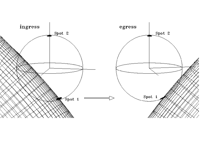
Figure 4: View of the system at phases of ingress and egress of spot 1 for the parameters of eclipse 1 for $q=0.2$ in Table 2. The secondary Roche lobe is projected as a wire model so that the white dwarf remains visible. The system inclination, $i$, where $i=0^{\circ}$ corresponds to pole-on, is inferred to be about $80^{\circ}$. The origin of the coordinate system is at the centre of the white dwarf, with the origin of co-latitude vertically ‘up’ (so that spot 2 has a co-latitude of close to $0^{\circ}$, while spot 1 is around $150^{\circ}$). The origin of longitude is the coordinate axis joining the line of centres, with increasing longitude in the direction of the third coordinate triad. Ingress or egress of a given spot constrains its instantaneous projected location on the plane of the sky to lie along the limb of the secondary at that instant. The combination of timings of both the covering and uncovering of a given spot then constrain its position in two dimensions.

3 Results and Discussion

3.1 Geometrical overview

Figure 2 displays a number of prominent features observed previously in UZ For through the optical (e.g. Allen et al. 1989; Bailey & Cropper 1991; Imamura & Steiman-Cameron 1998) to ultraviolet (Warren et al. 1995; Stockman & Schmidt 1996), and related to the variable viewing geometry with orbital phase (cf. Figure 8 of Ferrario et al. 1989; Figure 4 of Bailey & Cropper 1991; Figure 5 of Warren et al. 1995; Figure 7 of Stockman & Schmidt 1996). Most notable are the intensity variations out of eclipse and especially the pre-eclipse brightening, and the rapid changes during eclipse ingress and egress, attributable to the variable viewing geometry of the accretion spots and the accretion stream (e.g. Harrop-Allin et al. 1999; Kube et al. 2000).

Our present understanding of this system is illustrated in Figure 4, where the locations of the two accretion spots resulting from the present investigation are illustrated. The white dwarf is rotationally locked to the secondary, and eclipsed for about 8 min as the system rotates. Covering/uncovering of the white dwarf photosphere during ingress/egress occurs in about 40 s. The projected positions of the accretion spots on the plane of the sky are fully defined by the times of the successive rapid changes in light intensity as the spots themselves are covered and uncovered. If the position of the accretion spots are assumed to be located at the white dwarf surface, their location on the white dwarf is then defined by the inferred white dwarf radius. The rate of accretion affects the system brightness, and only at low accretion rates (i.e. in the low state) can emission from the white dwarf photosphere be distinguished (Bailey & Cropper 1991). The location of the emission regions probably depends on accretion rate: even it is assumed that the spin and magnetic field axes are aligned, the accretion spots can still be located away from the poles (e.g. towards the secondary) depending on where the ballistic flow impacts the field lines. With variable higher accretion rates, the accretion spots may therefore be expected to move accordingly.

3.2 System brightness

The optical light curve of UZ For is dominated by accretion flow onto the primary, and changes significantly from epoch to epoch. Imamura & Steiman-Cameron (1998) identify three states, ‘low’ (V$\sim 18.5$), ‘faint high’ (V$\sim 16.7$) and ‘bright high’ (V$\sim 15.9$), and provide a schematic representation of these. Our estimate of the magnitude of UZ For at the epoch of observation is derived from the observation of a $V=7.1$ mag star through a ND4 neutral density filter, resulting in 3300 detected photons^-1 over the array. With about 700 photons^-1 over the whole array from the sky, the sky-corrected signal in Figure 2 corresponds to a magnitude of about 17.7–18.1 mag out of eclipse, depending on phase, and ignoring the different spectral energy distributions of UZ For and the comparison star. At the time of our observations, the system therefore appears to be in an ‘intermediate’ state between the low state of Bailey & Cropper (1991) and faint high state of Imamura & Steiman-Cameron (1998).

In the low state, the light curve has an on-off appearance typical of a system accreting at a single point on the white dwarf, corresponding to the location of spot 1 in Figure 4. When this is not in view, the majority of the emission from the system at phases between $\phi\sim 0.15-0.65$ is from the two stellar photospheres. In the higher states, this phase interval is increasingly bright, until in the bright high state, the system is brightest at $\phi\sim 0.25$.

3.3 Shapes of eclipses and eclipse timing

The eclipse morphology of our data is distinct from that in the low and high states. Two pairs of rapid changes in brightness are prominent in all of our eclipses, around phases 0.97 and 1.03 (Figures 6 and 8), in contrast with the single active accretion pole observed by Imamura & Steiman-Cameron (1998). These can be assigned to the successive covering and uncovering by the secondary of two small accretion regions (‘spots’) on the surface of the white dwarf. These regions are resolved in our data at 0.5 s time resolution, with ingresses and egresses lasting $\sim$1.5 s (Figure 8). Such behaviour is also visible (but not discussed) in Bailey (1995), when the system is $\sim$1 mag brighter than the low state, and thus also in the intermediate state. The observations of Ferrario et al. (1989) were also in the intermediate state, but the time resolution of the data is insufficient to resolve rapid intensity changes through eclipse.

Bailey (1995) noted that the outer pair of rapid changes (spot 1, Figure 6) coincide in phase with the low state eclipse, and also with the simultaneous soft X-ray eclipse seen using ROSAT. This pair also coincide with the rapid changes in brightness in the faint high and bright high state data in Imamura & Steiman-Cameron (1998), the eclipses seen in the EUV by Warren et al. (1995), and those in the UV by Stockman & Schmidt (1996). Spot 2, in contrast, is not known to emit in X-rays.

Figure 5: Timing residuals with respect to our revised ephemeris (Equation 2) constructed from the eclipse timings in Bailey & Cropper (1991) and our present data (crosses). Also shown for comparison are the ROSAT timings from Ramsay (1994) (stars), and other timings in the literature (diamonds).

The shapes of the three eclipses in Figure 8 is similar. However, there are clear differences in the amplitude of the rapid brightness changes from eclipse to eclipse. Both spots are fainter in eclipse 3 compared to eclipse 1 and 4. There are also differences in the relative brightnesses at ingress and egress: the brightness change at ingress is larger for eclipse 1, while that at egress is larger for eclipse 4. In general however the relative spot total brightnesses are constant, with spot 1 $\sim$3 times brighter than spot 2. This indicates to first order that the relative accretion flow to each spot remains constant even in the presence of changes in the total flow rate.

In Table 1, we estimate the mid-points of each of these pairs of rapid changes in brightness for three of the four eclipses observed. For each eclipse, the outer drops ($t_{1}$ and $t_{4}$) are the most precipitous. There is no evidence for differences in these times as a function of energy, and our estimates of the mid-times are probably accurate to about 0.5 s. As noted in Section 2, our times have been formally transformed from UTC times of observation to TDB (barycentric dynamical time).

The eclipse ingress and egress durations for the spots in the three eclipses in Figure 8 are the same for each eclipse to within the measurement uncertainties. There is some evidence that the ingress duration for spot 1 is longer than the egress ($\sim$2 s as opposed to $\sim$1.5 s). These durations are similar to those in Bailey & Cropper (1991) (but where the time resolution was barely sufficient). The ingress and egress durations for spot 2 are only slightly less than those for spot 1 and of equal duration in the three eclipses, indicating a spot radius similar to that of spot 1. These durations are also consistent with upper limits in the EUV (Warren et al. 1995) and soft X-ray (Bailey 1995), of about 4.7 s and $\sim$5 s respectively.

Only in the low state of Bailey & Cropper (1991) is the white dwarf clearly detectable, and hence usable as a timing reference. Most UZ For studies (Warren et al. 1995; Imamura & Steiman-Cameron 1998) therefore use the spot 1 mid-eclipse point, corresponding here to the outer pair, $(t_{1}+t_{4})/2$, corrected to the centre of the white dwarf eclipse (by subtracting 9 s as appropriate for the $45^{\circ}$ longitude in Bailey & Cropper 1991), as the origin of zero phase. Eclipse 1 represents eclipse $67\,777$ (about 16 years) after the origin given by Imamura & Steiman-Cameron (1998). The cycle count is unambiguous, but our eclipses occur $\sim$100 s earlier than predicted by their quadratic ephemeris.

The eclipse timings in the literature (Ramsay 1994; Warren et al. 1995; Imamura & Steiman-Cameron 1998) show timing residuals of $\pm$50 s from the Imamura & Steiman-Cameron (1998) ephemeris. Part of the timing residuals may be attributable to motion of the spot on the surface of the white dwarf, for example as a result of changes in the accretion rate. However, these changes cannot amount to more than the eclipse duration of the white dwarf ($\sim$40 s), unless the emission originates far above the surface, and it seems unlikely that the more extreme residuals can be accommodated in this way. In view of the heterogeneous data, the large residuals with respect to the Imamura & Steiman-Cameron (1998) ephemeris, and the uncertainties in correcting to the centre of the white dwarf, we have derived a linear fit using only our high time resolution data (three eclipses) and that with the next best time resolution (from Bailey & Cropper 1991, six eclipses) to define a linear ephemeris:

$${\rm BJD}=2\,445\,567.17653(2)+0.0878654325(4)\,{\rm E}$$ (2)

where BJD is the barycentric Julian Date, E is the eclipse number and the uncertainties in brackets are in the last figure. The resulting fit (Figure 5) leads to residuals of less than 1 s for our data, less than about 4 s for the Bailey & Cropper 1991 data, and less than about 5 s for the ROSAT timings of Ramsay (1994). This suggests that the large residuals noted previously may result from timing errors (or untraceable time-scale inconsistencies) in these different datasets. High precision timing data will be important for future investigations of the spot longitude changes and correlations with accretion rate.

3.4 Geometrical interpretation

Our precise timing and high-speed photometric data allow the position of the accretion spots to be located on the plane of the sky (Figure 4). To locate them on the white dwarf, assuming that they originate at the surface, we require an estimate of the white dwarf radius. Working in terms of the system mass ratio, $q$, we trace the Roche potential out of the binary system along the line of sight from any point in the vicinity of the white dwarf. We then adjust the system parameters under the constraints of grazing contact of this line of sight with the Roche lobe at particular phases. Starting with the generally favoured $q=0.2$ solution of Bailey & Cropper (1991) to calculate the positions of the accretion regions on the white dwarf (corresponding roughly to $R_{\rm WD}\sim 8\times 10^{8}$ cm, and $M_{\rm WD}\sim 0.7\,M_{\odot}$, cf. Schwope et al. 1997), we recover the radius of the white dwarf and co-latitude of the spot seen in their data and given in their Table 2, to the level of accuracy recorded. The derived parameters are sensitive to small changes in inclination and white dwarf radius, and this is sufficiently accurate to ensure a common basis for the following comparisons.

Table 2:  Inclination and co-latitudes/longitudes of spots 1 and 2 as a function of mass ratio $q$, assuming both spots are in the hemisphere facing the secondary (however, see Section 3.7). Figure 4 should be consulted for coordinate definitions. Errors are estimated at the $1\sigma$ level.

Eclipse	Inclination	Spot 1		Spot 2
number		Co-lat	Long	Co-lat	Long
	(∘)	(∘)	(∘)	(∘)	(∘)
$q=0.15$
1	$82.7\pm 0.1$	$144\pm 3$	$31$	$0\pm 3$	$-3\pm 10$
3	$82.7\pm 0.1$	$149\pm 3$	$31$	$0\pm 3$	$-3\pm 10$
4	$82.7\pm 0.1$	$144\pm 3$	$31$	$0\pm 3$	$-3\pm 10$
$q=0.2$
1	$80.9\pm 0.1$	$150\pm 3$	$45$	$4\pm 3$	$-10\pm 7$
3	$80.9\pm 0.1$	$148\pm 3$	$45$	$4\pm 3$	$-10\pm 7$
4	$80.9\pm 0.1$	$150\pm 3$	$45$	$4\pm 3$	$-10\pm 7$
$q=0.3$
1	$78.5\pm 0.1$	$139\pm 3$	$45$	$11\pm 3$	$-10\pm 8$
3	$78.5\pm 0.1$	$144\pm 3$	$45$	$11\pm 3$	$-10\pm 8$
4	$78.5\pm 0.1$	$136\pm 3$	$45$	$11\pm 3$	$-10\pm 8$

We have measured the eclipse durations for spot 1 in our data, in the EUVE data of Warren et al. (1995), and in the ROSAT and optical data of Bailey (1995). As in Bailey & Cropper (1991) and other previous studies, we assume the accretion spots are located on the surface of the white dwarf. If we allow the phase to be a free parameter to accommodate the timing residuals against the ephemeris (see Section 3.3), spot 1 can be located at a co-latitude of $\sim$150^∘ and longitude of $\sim$45^∘ (ahead of the line of centres) from all these data, as in Bailey & Cropper (1991). The view at the phases of ingress and egress of spot 1 is shown in Figure 4. There is no evidence for any movement of this region in co-latitude ($<5^{\circ}$). Any longitude changes from epoch to epoch are mixed in with the timing uncertainties, so these are not possible to determine.

From our data for $q=0.2$ we locate spot 2 in the ‘upper’ hemisphere (that inclined towards the line of sight), at a co-latitude of $4^{\circ}\pm 3^{\circ}$ and a longitude of $-10^{\circ}\pm 7^{\circ}$ (Figure 4). A similar fit to the Bailey (1995) data yields $5^{\circ}\pm 3^{\circ}$ and a longitude of $-10^{\circ}\pm 12^{\circ}$. Spot 2 is therefore close to the rotation axis and slightly behind the line of centres, and at the same co-latitude at these two epochs.

UZ For provides the opportunity to obtain highly constrained fundamental system parameters in an interacting binary. We summarise the locations of the spots in Table 2 for $q=0.2$ and the other mass ratios in the range $0.15-0.3$ found to be acceptable by Bailey & Cropper (1991). For $q<0.15$ no solution is achievable for spot 2 unless it is above the surface of the white dwarf. In order to progress further with $q$, we have to update the mass-radius relationships used by Bailey & Cropper (1991). Recent measurements of white dwarf masses and radii for 40 Eri B (Shipman et al. 1997) and V471 Tau (Barstow et al. 1997) indicate close agreement with the Hamada-Salpeter mass-radius relation for He white dwarfs used by Bailey & Cropper (1991). Recent mass-radius data derived using Hipparcos parallaxes (Vauclair et al. 1997) do not add to the accuracy. No progress is therefore possible in the case of the primary. With respect to the secondary, both the period-mass relations of Warner (1995) and Patterson (1984) predict a secondary mass $M_{2}=0.17\,M_{\odot}$, consistent with $q=0.23$, while the Kolb & Baraffe (2000) ZAMS models predict a secondary mass of $M_{2}=0.24\,M_{\odot}$, consistent with $q=0.3$. Unless the secondary was significantly evolved at the onset of mass transfer (Kolb & Baraffe 2000), values of $q=0.2-0.3$ are to be preferred, implying $M_{\rm WD}=0.7-0.8\,M_{\odot}$. This would require the better fits to the white dwarf eclipse data in Bailey & Cropper (1991) at $q=0.15$ than $q=0.2$ to result from their neglect of limb darkening. This conclusion rests, however, on the reliability of the secondary period-mass relationship, which has been the subject of considerable discussion (see Warner 1995).

These locations are consistent with the spot eclipse ingress and egress durations (Section 3.3): as is evident from Figure 4 the projected dimensions of spot 1 are smaller in egress, leading to a shorter egress than ingress duration, as observed. On the other hand the projected dimensions of spot 2 are almost unchanged between ingress and egress, suggesting similar ingress and egress durations, again as observed. From the duration of the spot ingress and egress, we calculate that the angle subtended by either spot from the centre of the white dwarf in the dimension of the secondary limb travel is $3^{\circ}\pm 1^{\circ}$, in all eclipses. For a circular spot this translates to a fractional area of $7\times 10^{-4}$, consistent with the upper limit of $5\times 10^{-3}$ in Bailey & Cropper (1991).

Further progress in determining the parameters for this system is desirable and feasible by obtaining the highest quality measurements of the eclipse profile in the low state.

Figure 6: Sky-subtracted and flat-fielded total counts s^-1 (top), counts s^-1 in three bands 340–490 nm (labelled ‘B’ for ease of reference), 490–580 nm (‘V’) and 580–700 nm (‘R’), and two colour ratios constructed from the three energy-resolved light curves for eclipse 1. Lower values of these ratios imply a redder colour. Data are displayed in bins of 2 s for the intensities, and 5 s for the colour ratios, with error bars for the ratios corresponding to photon statistical errors. Orbital phase is with respect to the updated ephemeris given by Equation 2.

3.5 Colour variations

Figure 6 provides the background-subtracted energy-resolved light curves for eclipse 1, and also the two colour (hardness) ratios. For conciseness we refer to these as V:R and B:V ratios (from ‘red’, ‘visual’ and ‘blue’ based on the bandpasses in Figure 6). We also show the colour ratio changes in eclipses 3 and 4 in Figure 7. Eclipses 1 and 3 are similar, while the B:V ratio in eclipse 4 shows less variation than in the first two.

After both spots are eclipsed, the colour is significantly redder in the V:R ratio, in line with our expectation that the major contributor to the ‘red’ band at these phases is the secondary star. Although also redder at mid-eclipse, the B:V ratio has a somewhat different behaviour, generally decreasing to mid-eclipse and then increasing again. No significant change in colour is expected from the secondary during the narrow phase range spanned by the eclipse. This indicates that flux contributed by the secondary in these bands is less significant, as expected for a dwarf M star. The white dwarf and associated accretion regions on its surface will have been covered within $\sim$40 s of eclipse spot ingress (see Bailey & Cropper 1991), so by mid-eclipse the flux contributing to the colour change must be some distance from the white dwarf. The only obvious candidate is the accretion flow between the two stars. However, the approximately symmetrical B:V ratio change though eclipse is not easily reconciled with emission from a ballistic+magnetic trajectory to only spot 1. The stream to spot 2 is uncovered before spot 2 egress and when the stream to spot 1 is still eclipsed. It is therefore likely that the B:V colour variation is due to a combination of the progressive covering and uncovering of both streams.

Care is required in the interpretation of the colour changes during eclipse, as the background contribution (from, for example, the secondary star) affects the interpretation of the colour ratio changes. Nevertheless the colour ratios in Figure 6 provide evidence for significant changes at the time of the spot ingresses and egresses, in the sense that the V:R ratio becomes marginally bluer and the B:V ratio somewhat redder once spot 1 is eclipsed. This behaviour is repeated in eclipses 3 and 4 (although not in the B:V ratio for eclipse 4). It is possible to separate out with some confidence the contributions of each of the spots, stream and secondary in the three bands for the three eclipses. This indicates that the relative contribution of spot 2 in comparison to spot 1 is $0.52\pm 0.14$, $0.58\pm 0.10$ and $0.36\pm 0.03$ in the B, V and R bands at ingress and $0.54\pm 0.07$, $0.71\pm 0.16$ and $0.38\pm 0.15$ at egress respectively. Although there appear to be small differences in the colours from eclipse to eclipse, the statistical evidence for this is weak.

The relatively greater contribution in V may indicate that there are cyclotron humps in the spectrum of spot 2, not a broad continuum, and if so, is indicative of lower temperatures. Such humps have been seen out of eclipse by Ferrario et al. (1989) and Schwope et al. (1990), who found a lower magnetic field in spot 2 compared to spot 1, but it is unclear whether these can explain the relative flux distributions. An alternative explanation may lie in the different viewing angles to the two spots at the time of eclipse: spot 2 is seen almost face on, with bluer harmonics undergoing more absorption and scattering at these viewing angles (Wickramasinghe & Meggitt 1985), while spot 1 is seen almost side on.

There is also a slow general colour variation in the V:R ratio over the duration of the observations, with the source tending to become bluer towards the time of eclipse, although the colour changes more substantially during the eclipse itself. We can investigate whether the slow variation might originate from the ellipsoidal variation of the red light from the secondary (Ferrario et al. 1989). An upper limit for the emission from the secondary is available from the count rate near mid-eclipse, $\sim$4 per cent in R, which is therefore insufficient to cause the observed V:R ratio change. This suggests that the V:R change must be due to a difference in cyclotron flux distributions from the spots, either because of intrinsic differences, or because of different viewing angles to the spots at any one phase.

Figure 7: Sky-subtracted and flat-fielded colour ratios for eclipses 3 and 4, binned at 5 s (as for Figure 6).

In this context it is interesting to note that when spot 1 disappears over the limb at $\phi\sim 1.15$ ($\sim$5780 s in Figure 2) there is no significant colour change in V:R or B:V. This indicates that when viewing angles are similar, the apparent flux distributions are also similar, and so viewing angle differences to the two spots are likely to be the main cause of the slow variation in V:R outside of eclipse. Spot 2 is seen through a greater range of angles than spot 1, so this explanation is consistent with the fact that the V:R variation is symmetric about a point near the end of the eclipse, which is when spot 2 is seen most face on (Table 2).

There is a reduction in brightness before the eclipse at $\phi\sim 0.93$ (Figure 6, and $\sim$4200 s in Figure 2). Although from these optical data it is could be argued that the pre-eclipse dip is a photometric variation (see also Bailey & Cropper 1991), it is clear from EUV data (Warren et al. 1995) that the dip is caused by absorption in the stream crossing the line of sight to the accretion regions. The dip is almost grey, but slightly stronger in the blue. This is somewhat different from that seen in HU Aqr by Harrop-Allin et al. (1999), where the dip is strongest at red wavelengths. The almost grey colour of the dip indicates that the extinction must be caused mostly by electron scattering or by completely obscuring material, although the latter is unlikely throughout the stream cross section.

3.6 A search for high frequency variations in the light curves

Several AM Her systems have been observed to show quasi-periodic oscillations (QPOs) on time-scales of 1–2 s (Middleditch 1982; Larson 1987). Their origin in the shock region was conclusively demonstrated by Larson (1989) who found that QPOs were not observed when the shock region disappeared from view as it rotated behind the white dwarf. No evidence for QPOs has yet been found in UZ For (Imamura & Steiman-Cameron 1998). Our data allow us to search for evidence of QPOs with significantly higher sensitivity.

The data were split into several sections and the three energy bands defined, as previously noted, so that an approximately equal number of counts were present in each. A time binning of 0.2 s was used for each band. A Discrete Fourier Transform (DFT) was used to search for periodic signals in the data. No evidence for a QPO in any energy band was detected. We can set an upper limit for a strictly periodic signal of $\sim$0.5 per cent in each band. Since the power of a QPO is spread in frequency and not strictly periodic, it is more difficult to give an accurate upper limit for a QPO, but we expect this also to be $\sim$0.5 per cent.

The frequency of the shock oscillations depends sensitively on the local cooling rate within the shock, which varies with $\dot{M}$ and the magnetic field strength. In magnetic systems there are two competing cooling mechanisms in the accretion shock: thermal bremsstrahlung and cyclotron radiation. Chanmugam et al. (1985) showed that when cyclotron cooling was strong, the shock tended to be stabilised against oscillations. Further, Wu et al. (1996) found that the stabilising influence depends on the magnetic field strength: the higher the field strength the greater the stability. This was explored further by Saxton & Wu (1999). In the case of UZ For, Schwope et al. (1990) found that the main accretion pole had a field strength of 53 MG and the secondary pole a field strength of 75 MG. This would suggest that cyclotron emission is the dominant cooling process in each accretion region and the shock is relatively stable – as confirmed by these observations.

3.7 Behaviour in different brightness states

We now consider the origin of the different photometric behaviour at different brightness states of the system.

The low state maximum is $\sim$0.1 of the bright high state maximum, indicating a substantial increase in emission in the higher states, particularly at those phases $\sim$0.15–0.65 when spot 1 is out of view. Spot 2 is in view between $\sim$0.75–0.35, with maxima expected from cyclotron beaming (Wickramasinghe & Meggitt 1985) at phases 0.85 and 0.25, or at phase 0.05, depending on the spot co-latitude. Some of the additional contribution in the bright high state could therefore come from this spot, but not the majority because spot 2 is at most only weakly evident in the eclipse profiles in Figures 7 and 8 of Imamura & Steiman-Cameron (1998).

Figure 8: The white light ingresses and egresses of eclipses 1, 3 and 4 at 0.5 s time resolution (see Table 1). Each successive eclipse is displaced vertically by 2000 counts s^-1. Orbital phase is with respect to the updated ephemeris given by Equation 2.

These considerations, and the phasing of the slow increase after spot 1 egress in the bright high state data, can only arise, as argued by Imamura & Steiman-Cameron (1998), from an extended emission structure leading the line of centres – probably the accretion stream to spot 1. At ingress, spot 1 is itself $\sim$5 times brighter than it was in the low state ($\sim$2 times at egress). Imamura & Steiman-Cameron (1998) note that the accretion stream is at least as bright as spot 1 at ingress, and significantly brighter than any contribution from spot 2 that might be buried in their light curves. Given that spot 1 will have passed out of view over the limb at phase 0.15, and given the absence of strong emission from spot 2, almost all of the emission in the bright high state at phase 0.25 (at which phase the system is at its brightest) must be from the stream.

The rotation of spot 1 over the limb should cause a change in brightness. None of our observations covers the phases when the spot rotates into view, but the rotation out of view is covered in Figure 2 at $\sim$5780 s, where a decline in brightness is evident. The decline is more gradual than that observed at blue wavelengths in Bailey & Cropper (1991), but is at a similar phase. Bailey & Cropper (1991) state that the duration of the bright phase, when spot 1 is in view, is consistent with the latitude and longitude they derive for the spot for $q=0.2$. This is true only if the optically emitting region is a small height above the surface of the white dwarf ($0.025R_{\rm WD}$), as expected for the standard accretion scenarios (see Cropper et al. 1999). The decline in brightness at $\sim$5780 s in Figure 2 is also consistent with the latitudes and longitudes we derive in Table 2, for all values of $q$ tabulated, if we assume a height of $0.02-0.025R_{\rm WD}$ (a more precise height determination is prevented by the gradual nature of the decline in our data). The height of the region depends in an inverse manner on the local accretion rate. The more gradual decline in our data may therefore be a result of a slightly lower height caused by the higher accretion rate in the intermediate state. The smaller drop in brightness compared to the spot brightness at eclipse egress can be qualitatively explained by the beaming of the cyclotron radiation and by an increase in the contribution of the accretion stream as it is viewed increasingly side-on.

It may be questioned whether the decline at $\sim$5780 s is in fact the signature of spot 1 rotating over the limb. In order to remain in view, the consequence would be that the height of the optically emitting region must be significantly higher, requiring a change in spot latitude and a different inclination from those derived in Table 2 and in Bailey & Cropper (1991). It is also questionable whether a small localised region of emission, consistent with both ingress and egress spot eclipse durations, is physically possible at heights far above the white dwarf. We therefore prefer the interpretation that the decline at $\sim$5780 s is due to the rotation of spot 1 over the limb.

We conclude the following: in the low state there is no evidence for spot 2 or an accretion stream to spot 1; in the intermediate state accretion begins at spot 2 and some stream becomes evident (whether to spot 1 or 2 must be subject to more detailed modelling); in the faint high and bright high states the accretion increases at spot 1, and the stream becomes brighter still. This indicates that in the optical the stream brightness is strongly dependent on the accretion rate – more so than the spot brightness.

It is also evident that the emission from spot 2 is greatest in the intermediate state and that it does not increase commensurately with the emission from spot 1 at higher accretion rates. In the higher states at the time of the EUVE observations (Warren et al. 1995) there is no evidence for spot 2 in the EUV. In the intermediate state when spot 2 is clearly visible in the optical, there are no detectable X-rays in the ROSAT soft or hard bands (Bailey 1995).

While the reduction in emission from spot 2 in the brighter states can be explained by changes in the accretion stream trajectory at higher accretion rates, it is difficult to explain the absence of soft or hard X-rays from spot 2 (Bailey 1995) in the intermediate state. One possibility could be that the foot of the accretion region is behind the limb of the primary at the time it is eclipsed, with only the top (optical cyclotron emitting) of the postshock accretion flow visible above the limb. In order to be consistent with the phasing of spot 2 ingress and egress, the co-latitude would be limited to only a few degrees more than $90^{\circ}-i$, the longitude must be $180^{\circ}$: no solution is obtainable for the $q=0.3$ case, and it is marginal for the $q=0.2$ case. For $q=0.15$ a solution with a co-latitude of $11^{\circ}$ and an emitting height above the white dwarf surface of $0.025\,R_{\rm WD}$ is consistent. This has the advantage of naturally explaining the disappearance of the second spot at higher accretion rates (when the post-shock region cools more efficiently and is lower). On the other hand we have argued in Section 3.1 that mass ratios in the range $0.2-0.3$ are to be preferred if we accept the constraints of the secondary star period-mass relationships, and the special conditions of a grazing occultation of the accretion column may be considered unlikely.

We suggest instead that the accretion rate at spot 2 is low enough that no accretion shock forms: instead the accreting material interacts with the white dwarf surface layer directly (the ‘bombardment solution’ of Kuijpers & Pringle 1982). This has been investigated for parameters appropriate to UZ For by Woelk & Beuermann (1992), with the prediction that the optical flux produced by cyclotron radiation is sufficient to produce the observed spot brightness ($\sim 0.05$ mJy). At the same time the temperature in the optically thick atmospheric layers emitting X-rays is $\sim 10$ eV, too low to be detected in the ROSAT band, even for the low interstellar absorption to this system (Ramsay et al. 1994).

4 Conclusions

The high time resolution, quantum efficiency, dynamic range and intrinsic colour resolution of the new STJ detector has made it possible to explore the accretion processes in even faint magnetic cataclysmic variables with new levels of precision. The photon-counting nature of the instrument allows the data to be combined flexibly, a posteriori, in spectral and temporal bins limited only by the photon statistics, while the limited array size is nevertheless sufficient to provide simultaneous sky subtraction.

We have obtained data for three eclipses of UZ For. We attribute two sharp changes in brightness to the eclipse of two small accretion regions and localise them on the surface of the white dwarf primary. The first of these is at the lower hemisphere at the location seen by others in the optical (e.g. Bailey & Cropper 1991), and in the EUV and X-rays (Warren et al. 1995; Bailey 1995). The second is in the upper hemisphere, near the rotation axis, and there is no evidence for any emission from this region in X-rays. We have explained this in terms of the bombardment solution of Kuijpers & Pringle (1982) which produces optical emission from a thin interaction layer, while requiring the X-ray emission to be sufficiently cool to be unobservable by ROSAT. However, we also have to consider the possibility of a grazing occultation of this region, although the special conditions required are somewhat unsatisfactory.

We have updated the orbital ephemeris using those timings we believe to be of the highest accuracy. This will be important for future investigations of the spot longitude changes and correlations with accretion rate. Light time corrections to the Solar System barycentre are required to obtain timing accuracies below $\sim$3 s, which is significant in comparison with the diameter of the white dwarf of $\sim$40 s.

The accretion regions are resolved in our data, and we derive a spot size as a fraction of the white dwarf surface of slightly less than $10^{-3}$, somewhat smaller than the size usually derived for accretion spots in optical data. This may result partly from a lower time resolution and S/N ratio in other data compared to that available here.

We have looked for, and placed strong upper limits on, QPOs on time-scales of order 1 s, as seen in some other AM Her systems. We conclude that the magnetic field and thus cyclotron emission is sufficient to stabilise the post-shock flow (Saxton & Wu 1999).

An analysis of the accretion spots and the accretion stream brightness, along the lines of that in Harrop-Allin et al. (1999), is planned for a subsequent paper. Significantly higher spectral resolution STJ data expected in the future would be well matched to obtain low-resolution cyclotron spectra in AM Her systems. By co-adding several eclipses, it will be possible to obtain this spectral data even for short phase intervals, e.g. after eclipse ingress of spot 1 and before that of spot 2. In brighter systems a reconstruction of the accretion spot will be possible in several spectral bands.

References

- Allen et al. (1989) Allen R. G., Berriman G., Smith P. S., Schmidt G. D., 1989, ApJ, 347, 426
- Bailey (1995) Bailey J., 1995, in Buckley D. A. H., Warner B., eds, Cape Workshop on Magnetic Cataclysmic Variables Fundamental properties of polars. ASP Conf. Ser. 85, San Francisco, pp 10–20
- Bailey & Cropper (1991) Bailey J., Cropper M., 1991, MNRAS, 253, 27
- Barstow et al. (1997) Barstow M. A., Holberg J. B., Cruise A. M., Penny A. J., 1997, MNRAS, 290, 505
- Blackburn (1995) Blackburn J., 1995, in Shaw R. A., Payne H. E., Hayes J. J. E., eds, Astronomical Data Analysis Software and Systems IV FTOOLS: A FITS data processing and analysis software package. ASP Conf. Ser. 77, San Francisco, pp 367–370
- Chanmugam et al. (1985) Chanmugam G., Langer S. H., Shaviv G., 1985, ApJ, 299, L87
- Cropper (1990) Cropper M., 1990, Space Sci. Rev., 54, 195
- Cropper et al. (1999) Cropper M., Wu K., Ramsay G. T., Kocabiyik A., 1999, MNRAS, 306, 684
- Ferrario et al. (1989) Ferrario L., Wickramasinghe D. T., Bailey J., Tuohy I. R., Hough J. H., 1989, ApJ, 337, 832
- Harrop-Allin et al. (1999) Harrop-Allin M. K., Cropper M., Hakala P. J., et al., 1999, MNRAS, 308, 807
- Imamura & Steiman-Cameron (1998) Imamura J. N., Steiman-Cameron T. Y., 1998, ApJ, 501, 830
- Kolb & Baraffe (2000) Kolb U., Baraffe I., 2000, New Astron. Rev., 44, 99
- Kube et al. (2000) Kube J., Gänsicke B. T., Beuermann K., 2000, A&A, 356, 490
- Kuijpers & Pringle (1982) Kuijpers J., Pringle J. E., 1982, A&A, 114, L4
- Kusters (1996) Kusters J. A., 1996, Hewlett-Packard Journal, December 1996, 60
- Larson (1987) Larson S., 1987, A&A, 181, L15
- Larson (1989) Larson S., 1989, A&A, 217, 146
- Middleditch (1982) Middleditch J., 1982, ApJ, 257, L71
- Osborne et al. (1988) Osborne J. P., Giommi P., Angelini L., Tagliaferri G., Stella L., 1988, ApJ, 328, L45
- Patterson (1984) Patterson J., 1984, ApJS, 54, 443
- Peacock et al. (1996) Peacock A., Verhoeve P., Rando N., et al., 1996, Nature, 381, 135
- Peacock et al. (1997) Peacock A., Verhoeve P., Rando N., et al., 1997, A&AS, 123, 581
- Perryman et al. (1999) Perryman M. A. C., Favata F., Peacock A., Rando N., Taylor B. G., 1999, A&A, 346, L30
- Perryman et al. (1993) Perryman M. A. C., Foden C. L., Peacock A., 1993, Nuc. Inst. Meth. A, 325, 319
- Ramsay (1994) Ramsay G., 1994, IBVS, 4075
- Ramsay et al. (1994) Ramsay G. T., Mason K. O., Cropper M., Watson M. G., Clayton K. L., 1994, MNRAS, 270, 692
- Rando et al. (1998) Rando N., Peacock A., Andersson S., et al., 1998, Proc. SPIE, 3435, 74
- Rando et al. (2000) Rando N., Verveer J., Verhoeve P., Peacock A., et al., 2000, Proc. SPIE, ATI-2000, Munich, in press
- Saxton & Wu (1999) Saxton C. J., Wu K., 1999, MNRAS, 310, 667
- Schwope et al. (1990) Schwope A. D., Beuermann K., Thomas H.-C., 1990, A&A, 230, 120
- Schwope et al. (1997) Schwope A. D., Mengel S., Beuermann K., 1997, A&A, 320, 181
- Shipman et al. (1997) Shipman H. L., Provencal J. L., Høg E., Thejll P., 1997, ApJ, 488, 43
- Stockman & Schmidt (1996) Stockman H. S., Schmidt G. D., 1996, ApJ, 468, 883
- Vauclair et al. (1997) Vauclair G., Schmidt H., Koester D., Allard N., 1997, A&A, 325, 1055
- Warner (1995) Warner B., 1995, Cataclysmic Variable Stars. Cambridge University Press
- Warren et al. (1995) Warren J. K., Sirk M. M., Vallerga J. V., 1995, ApJ, 445, 909
- Wickramasinghe & Meggitt (1985) Wickramasinghe D. T., Meggitt S. M. A., 1985, MNRAS, 214, 605
- Woelk & Beuermann (1992) Woelk U., Beuermann K., 1992, A&A, 256, 498
- Wu et al. (1996) Wu K., Pongracic H., Chanmugam G., Shaviv G., 1996, Publ. Astron. Soc. Australia, 13, 93