Lensing by Lyman Limit Systems:
Determining the Mass to Gas Ratio

Abstract

We present a new method to determine $\Upsilon_{\rm HI}$, the total mass-to-neutral gas ratio in Lyman-limits systems. The method exploits the relation between the neutral hydrogen column density and the magnification of background sources due to the weak gravitational lensing that these systems induce. Because weak lensing does not provide a direct measure of mass, one must use this relation in a statistical sense to solve for the average $\Upsilon_{\rm HI}$ and its distribution. We use a detailed mock catalog of quasars (sources) and Lyman-limit systems (lenses) to demonstrate the applicability of this approach through our ability to recover the parameter $\Upsilon_{\rm HI}$. This mock catalog also allows us to check for systematics in the method and to sketch its limitations. For a universal constant $\Upsilon_{\rm HI}$ and a sample of $n_{\rm QSO}$ quasars, we obtain an unbiased estimate of its value with $95\%$ confidence limits (independent of its actual value) of $\Upsilon_{\rm HI}\pm 140\,\sqrt{10^{5}/n_{\rm QSO}}$.

1 Introduction

The Lyman limit systems of neutral hydrogen column density ${\rm N_{HI}}>2\times 10^{17}{\rm{cm}^{-2}}$ are believed to be closely related to galaxies at all redshifts. Among these the rare damped ${\rm Ly-}\alpha~{}$systems (DLAS) with ${\rm N_{HI}}>2\times 10^{20}{\rm{cm}^{-2}}$ are usually identified with galactic disks (Wolfe et al. (1986); see, however, Rauch et al. (1997)), while lower column density systems are more likely to correlate with galactic or proto-galactic halos (Bahcall & Spitzer, 1969; Churchill et al., 1996; Mo & Miralda-Escude, 1996; Abel & Mo, 1998). Halos are the basic building blocks of structure formation when it comes to dark matter (DM) gravitational collapse and virialization in any hierarchical scenario. Hence, low column density Lyman limit systems (hereafter simply LLS) provide a unique opportunity to study the connection between the DM component and the gas component at different redshifts while the two are still in hydrodynamical equilibrium.

The relation between the DM component and the gas component in LLS can be characterized in terms of the “mass-to-gas” ratio, in analogy to the mass-to-light ratio commonly used for galactic disks. In the large scale structure picture this ratio represents the mean value of the biasing factor, which connects the spatial distribution of the baryons (gas as well as stellar disks) with that of the dark matter. Generally, the biasing may be a linear relation between the gas over-density and the DM over-density, or a more elaborated functional connection (e.g., Dekel & Lahav 1999). Biasing can be deterministic, but in reality it is more likely to be stochastic. It is possible to calculate such parameters as the mean biasing in any scheme in which there is a functional relation between the bias and the overdensity.

In order to determine the mass-to-gas ratio, one has to observe at least two quantities, where one of them is directly related to the gas density and the other probes the DM density field. This has been in part applied by Croft et al. (1998) who presented a method by which they recover the DM density fluctuations from the ${\rm Ly-}\alpha~{}$forest. A detailed comparison to $N$-body  simulations provided them with the “experimental” bias parameter and spared the need to solve for it independently. Based on these simulations, Katz et al. (1996) and Hernquist et al. (1996) previously realized that ${\rm Ly-}\alpha~{}$absorption systems consist of a variety of physical objects: collapsing halos, cusps in phase space for density shells, and galactic disks. The nice agreement between the results from the simulations and the observed column density function added credibility to this picture.

The appeal to $N$-body  simulations can be computationally expensive, and it is unclear whether the higher resolution needed for the LLS can be achieved today in a large cosmological simulation (Gardner et al., 1999). The simulations also make assumptions on the physical conditions and the equation of state of the gas, which also limits their use. It is therefore desirable to construct an independent method by which the mean mass-to-gas ratio and other parameters can be measured.

Here we propose to use gravitational lensing to determine the matter content, baryonic fraction and ionization state of the LLS. The absorption features, being a direct probe of the neutral hydrogen content in LLS, provide complementary data needed to reveal the connection between the matter and HI densities.

The absorption features are well known and well measured (see Petitjean, 1998; Rauch, 1998, for recent reviews). Their interpretation, although subject to uncertainties in fitting the line profile, is rather straightforward and can be expressed in terms of their column density ${\rm N_{HI}}$, their equivalent width, and their velocity parameter. The lensing due to the moderate column densities of the LLS has not previously been considered because of the low signal expected.

So far only lensing by DLAS (${\rm N_{HI}}>2\times 10^{20}{\rm{cm}^{-2}}$) has been studied for its effect on the magnification bias for the background source population, as well as on the distribution of the observed impact parameters with respect to the center of the lens (Smette et al., 1997; Bartelmann & Loeb, 1996; Smette, 1995). Lensing by column densities of ${\rm N_{HI}}<10^{20}{\rm{cm}^{-2}}$ seemed unreasonable to consider because of the very small effect it has on the background sources; a typical quasar is only magnified by about one percent. Theoretically, only the overall effects of lensing on quantities like the luminosity function of quasars have been considered (Hamana et al., 2000; Pei, 1995a), while observationally a possible excess in the number counts of metal line systems has been detected (vanden Berk et al., 1996).

Other manifestations of weak lensing have been detected and used to map the mass distribution in clusters and larger scale structure (see Bartelmann & Schneider 2000 for a review). The standard lore in weak gravitational lensing is to use the ellipticity as induced by the intervening gravitational shear field in order to resolve the projected mass distribution along the line of sight (Kaiser & Squires, 1993). Due to the small level of magnification and the unavailable absolute luminosity of the sources, the observed flux of the background sources has never been used in weak lensing studies. For this reason, point sources, for which ellipticities cannot be measured, cannot be used to map intervening mass concentrations in this fashion. The weak magnification of point sources has usually been considered only as a nuisance in extracting information from the background sources (e.g., in the case of supernovae Ia Wambsganss et al., 1997; Porciani & Madau, 2000).

Until now, a key aspect of the phenomenon of weak lensing by LLS has been neglected, the fact that the same systems that cause the magnification are also responsible for the troughs in the continuum emission of the background source. Both are proportional to projected surface densities along the line of sight. The two are therefore correlated. It is this correlation, and the fact that it holds for each individual system that we wish to exploit in order to extract statistically the relation between the total mass of these systems and their HI content. In addition, the absorption system gives the redshift of the lens.

In a large sample, the magnification of point sources can have a strong statistical effect. Treating all quasars as a set eliminates in part the need to know the absolute magnitudes of the individual sources. The magnification shifts the luminosity function of the combined population in a calculable way. The lensed population can be “de-magnified” (assuming a mass-to-gas scheme) on an individual basis. The criterion for a successful correction is the return to the statistical properties of an un-lensed population.

Every statistical approach requires a large data base in order to maximize the signal to noise ratio. Fortunately in the upcoming years such a data base will become available when the quasar sample from the Sloan Digital Sky Survey (SDSS) is completed. This sample should serve as an excellent target list by itself or for follow-up observations. Combined with high resolution spectra for a selective sub sample from ground- and space-based telescopes it will allow coverage of ${\rm Ly-}\alpha~{}$absorption features over a wide range of redshifts.

Here, we propose a recipe for an observational project to determine the mass-to-neutral-hydrogen ratio in LLS, check different bias schemes, or apply a similar technique to the mass-to-metal-line ratio in these systems.

In §2 we define our notation and present the formalism of the technique. In order to describe the main features of the proposed method in §3, we introduce a toy model which avoids many complications and which allows us to outline the ingredients of the technique. The next section (4) is devoted to the generation of a realistic mock quasar and Lyman-limit system catalog which enables various estimates of the method’s biases and errors, as well as the functional dependence of the obtained signal-to-noise ratio on the input parameters. In the same section, we use Monte-Carlo realizations of that catalog and describe our procedure for measuring the mass-to-gas ratio. The method is implemented, and its advantages and limitations are discussed. We conclude this section by additional checks that verify that the measured effect indeed comes from gravitational lensing. In section 5 we sketch the preferred procedure for actual observations, consider extensions of the method, and estimate additional effects like dust. Section 6 summarizes the method’s strengths and weaknesses.

2 The Theory

It is common in gravitational lensing to express the magnification in terms of two dimensionless quantities; $\kappa$, the convergence and $\gamma$, the shear. The magnification $\mu$ is then given by

$$\mu={{1}\over{(1-\kappa)^{2}-\gamma^{2}}}\,,$$ (1)

(Narayan & Bartelmann, 1999; Schneider et al., 1992). In the weak lensing limit, where $\kappa\sim\gamma\ll 1$ this equation becomes

$$\mu=1+2\kappa\,.$$ (2)

The convergence, $\kappa$, is the projected surface density, $\Sigma$, along the line of sight divided by the critical surface density,

$$\Sigma_{\rm cr}={{c^{2}}\over{4\pi G}}D_{\rm eff}\,;\,D_{\rm eff}={{D_{l}D_{ls}}\over{D_{s}}},$$ (3)

where $D_{l,s,ls}$ are the angular diameter distances between observer, lens and source.

For absorption systems the column density in neutral hydrogen, ${\rm N_{HI}}$, along the line of sight is related to $\Sigma$ via

$${\rm N_{HI}}={\rm Y}_{\rm HI}{f_{\rm H}\over m_{\rm H}}f_{b}f_{g}\Sigma\,,$$ (4)

where $f_{\rm H}$ the fraction of baryons that are in hydrogen, $m_{\rm H}$ is the hydrogen mass, $f_{b}$ is the fraction of total mass made up by baryons, and $f_{g}$ is a geometry factor that relates the possible different geometries of the baryons and the dark matter (e.g., gas disk in a spherical dark matter halo, etc.). The fraction of neutral hydrogen is defined by

$${\rm Y}_{\rm HI}={\rho_{\rm HI}\over\rho_{\rm H}}={{\rm N_{HI}}\over{\rm N}_{\rm H}}\,,$$ (5)

where in the last equality we explicitly assume that the volume density fraction is identical to the surface density fraction. The geometry factor, $f_{g}$ is of order unity if LLS can be adequately described by a roughly spherical halo with the DM and baryons well mixed.

We can define a projected mass-to-gas ratio,

$$\Upsilon_{\rm HI}\equiv{{\Sigma}\over{m_{\rm HI}{{\rm N_{HI}}}}}\,,$$ (6)

which is determined by these different factors. Observations suggest values of $f_{b}\sim 0.1$ (Kirkman et al., 2000), $f_{\rm H}\simeq 0.75$, and ${\rm Y}_{\rm HI}$ in the range of $10^{-2}-10^{-3}$ for $z=0-5$ (Prochaska, 1999; Haardt & Madau, 1996). Hence from Eqs. (4) and (6) we expect $\Upsilon_{\rm HI}$ to be in the range of $10^{2}-10^{4}$.

In a similar manner it is possible to define a mass-to-ionic-column-density ratio that relates the magnification to a metal line column density. This introduces an additional parameter, the metallicity of the gas, or, more accurately, the specific abundance of a certain metal in a specific ionization state. Throughout this paper, except in §5, we will focus specifically on HI absorption. However, everything we will present can also be applied to any observed metal line.

With the above definitions we can now express the magnification of a quasar by an absorption system along its path as

$$\mu=1+2{\Upsilon_{\rm HI}{\rm N}_{\rm HI}m_{\rm H}\over\Sigma_{cr}}.$$ (7)

If we could measure the magnification of a single quasar, we could determine $\Upsilon_{\rm HI}$ for every observed absorption system. However since there is no way to know a quasar’s un-lensed luminosity, we must exploit the correlation between magnification and the observable ${\rm N_{HI}}$ to determine $\Upsilon_{\rm HI}$ statistically.

For a statistical sample of quasars, magnification has two effects. It causes the observed solid angle to correspond to a smaller solid angle in the source plane, and therefore the density of quasars with fluxes intrinsically above a flux limit decreases. However, magnification also increases the flux received from each quasar and therefore more quasars are detected above the flux limit. The net effect depends on the slope of the luminosity function of quasars. An increase in the number of quasars is detected if the slope is steeper than $-2$ and a decrease otherwise. In the situation we will be considering, magnification will tend to increase the number of quasars brought into a sample.

In the next section, we illustrate the essence of the effect studied here with a toy model. Most of its simplifications will be dropped in later sections, to which readers familiar with gravitational lensing might want to skip right away.

3 Simple Model

In this section we introduce a simple model that demonstrates the basic concepts of the method for a statistical recovery of $\Upsilon_{\rm HI}$ without the complications that will be introduced in the following, more realistic case.

Let us assume all quasars are at $z=3$ and their luminosity function (LF) is given by a power law of slope $-3.0$. The number of absorption systems as a function of column density and redshift with column densities in the range $18<\log{\rm N_{HI}}<19.7$ is taken to be

$${\rm d}n=0.096{\rm N}_{18}^{-1.5}(1+z)^{1.55}{\rm d}{\rm N}_{18}{\rm d}z$$ (8)

where ${\rm N}_{18}={\rm N_{HI}}/(10^{18}{\rm{cm}^{-2}})$. The choice of these parameters will be justified in section 4.1. Throughout this paper we adopt the cosmological parameters ${\rm H}_{0}=65\,{\rm{km\,s}}^{-1}{\rm{Mpc}}^{-1}$, $\Omega_{M}=0.3$ and $\Omega_{\Lambda}=0.7$.

Using these distribution functions, we construct a sample of quasars and the associated absorption line systems along their lines of sight. The magnification value for each quasar is calculated according to the systems in its foreground, and the apparent luminosity of the quasar is correspondingly corrected by applying Eq. 7. The dilution of quasars by solid-angle magnification is taken into account by randomly removing quasars. This is performed for values of $\Upsilon_{\rm HI}$ of $0$, $1000$, and $2000$ (we loosely denote the un-lensed case by $\Upsilon_{\rm HI}=0$).

A flux cutoff at 45 $\mu$Jy (B brighter than $20^{m}$) is then applied to the magnified sample. Quasars which initially were below this flux limit are magnified by their LLS, exceed the flux limit, and introduce more high column density systems into the sample.

Figure 1: The observed luminosity function of our toy model for all quasars and for quasars with at least one absorption system with $\log{{\rm N_{HI}}}>19.0$. Each is plotted for three values of $\Upsilon_{\rm HI}$ (0, 1000, 2000). The upper three lines lie on top of each other as weak lensing has a negligible effect on the total quasar luminosity function, as was previously found. However the magnification by gravitational lensing is discernible in the subset of quasars that contain high column density absorption systems.

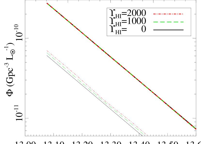
Figure 1 shows the quasar LF in this toy model. The upper lines depict the LF of all quasars in the sample with the three $\Upsilon_{\rm HI}$ values. Since the fraction of significantly magnified quasars is negligible, the magnification (different $\Upsilon_{\rm HI}$ values) has no detectable effect on the total LF, in accord with the conclusions of Pei (1995a). The lower three lines depict the LF as derived from a subset of quasars with at least one absorption system with $\log{\rm N_{HI}}>19.0$. For this subset it is evident that the LF is shifted to the right with increasing $\Upsilon_{\rm HI}$, i.e. increasing magnification.

In principle, the relative heights of the different lines in Fig. 1 are proportional to $\Upsilon_{\rm HI}$ and could be used to find its value. Unfortunately, in practice there is only one realization of the Universe so only one of the lines (for each ${\rm N_{HI}}$ cutoff) in Fig. 1 is observed. In order to find out what is the relative amplitude, the lowest line (un-lensed, $\Upsilon_{\rm HI}=0$) should be inferred from the expected fraction of high column density systems, based on lower column density systems and Eq. (8). Thus the effect of magnification is to change the fraction of observed quasars with high column density absorption systems.

Figure 2: The distribution of column densities of observed absorption systems for values of $\Upsilon_{\rm HI}$ of 0, 1000, and 2000. The number of absorption systems observed per 1000 quasars is plotted versus the log of the column density. For higher values of $\Upsilon_{\rm HI}$ more high column density systems are brought into the sample because of the magnification bias on the background sources.

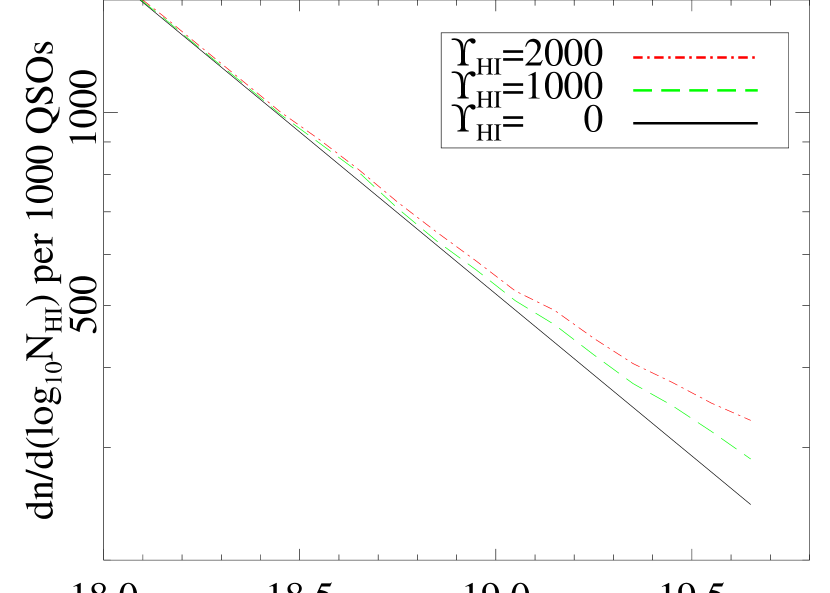
This effect is more clearly seen if instead of looking at the luminosity function we look at the distribution in column density of the absorption systems. Figure 2 shows this distribution for different values of $\Upsilon_{\rm HI}$. The effect of increasing $\Upsilon_{\rm HI}$ is immediately obvious; more high column density systems are brought above the flux limit due to magnification bias. The distribution also deviates from the original power law as the effect becomes progressively more pronounced with increasing ${\rm N_{HI}}$.

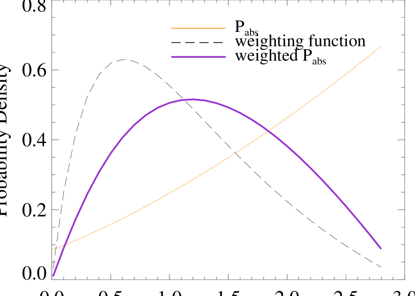
The magnification which causes the line divergence in Fig. 2 is not only a function of $\Upsilon_{\rm HI}$ but also of the lens’ redshift through $D_{\rm eff}$ in Eq. (3). We demonstrate this dependence in Figure 3 where the probability of encountering an absorption system (here normalized to integrate to unity) as given by Eq. (8) is weighted by the redshift dependent factors of Eq. (3) that contribute to the magnification. The resultant function is a modification of Eq. (8) (again normalized to integrate to unity) with a broad distribution in redshift. This means that lensing by absorption systems is relevant over a wide range of redshifts.

Figure 3: Magnification weighted probability of an absorption system as a function of absorption redshift (thick solid line) for quasars at $z=3$. The unweighted probability of an absorption system (Eq. 8, thin dotted line is weighted by $D_{\rm eff}$ of Eq. (3) (dashed line). All three functions are normalized so that they integrate to unity. The combination of magnification weighting which peaks at intermediate redshifts, and a monotonically increasing probability of encountering an absorption system with redshift, results in a rather broad redshift range in which lensing by absorption systems is important.

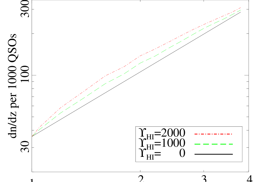
This redshift dependence distinctly affects the counts of absorption systems per unit redshift for a fixed number of quasars. This effect depends on the value of the magnification coefficient, $\Upsilon_{\rm HI}$. Figure 4 shows the number of absorption systems with $\log{\rm N_{HI}}>19.0$ as a function of absorption redshift. The increase in number of high column density absorption systems happens preferentially between redshifts of 0.5 and 2.0. This is a clear sign that the increase is due to lensing for which the magnification becomes very small as the lens approaches the quasar redshift. A deviation from the redshift power-law dependence of Eq. (8) is thus a statistical tool by which the amplitude of the magnification can be inferred. These effects do depend to some extent on cosmology.

Figure 4: The distribution of observed absorptions systems with column densities greater then $10^{19}{\rm{cm}^{-2}}$ in redshift for $\Upsilon_{\rm HI}$ values of 0, 1000 and 2000 for quasars at $z=3$. Since lensing depends on the redshift of the lens, systems that are at redshifts between 0.5 and 2.0 are preferentially brought into the sample.

The toy model we have used here highlights the main effects of treating the magnification by intervening absorption line systems in a statistical manner. The luminosity function of quasars is shifted to higher luminosities, a shift that can be observed if a cut by column density along their line of sight is performed. However, it is cumbersome to get a reference line for a non-lensed luminosity function, whereas it is more straightforward to detect the change in the column density function and its redshift distribution.

4 Recovery method for $\Upsilon_{\rm HI}$

The results of the toy model as presented in the last section portrayed the basic effects of lensing on the statistical distributions of quasars and their absorption systems. In reality, however, there are various deviations from the idyllic picture of the toy model. In order to assess our ability to use these altered distributions for the recovery of $\Upsilon_{\rm HI}$ we need to take all of these complications into account. Only a detailed imitation of a realistic situation will allow us to draw conclusions regarding the success or failure of the recovery method.

The main complications that should be included in a more realistic picture are;

• The observed luminosity function of quasars resembles a double power law, rather than a single one, and thus an additional scale (the “knee”) is added to the problem (Boyle et al., 1988; Hartwick & Schade, 1990; Warren et al., 1994; Boyle et al., 2001).

• The observed quasars span a large range of redshifts. This together with the redshift dependence of the LF “knee” results in a complicated observed flux function.

• An observed sample is flux limited, but quasars may be magnified above the flux limit depending on their absorption systems and the value of $\Upsilon_{\rm HI}$.

• Frequently, more than one absorption system intersects the line of sight to a quasar. These events, especially for high column densities, contribute a substantial signal to the shifts of the distribution functions. Multiple magnification events must thus be included in the analysis.

• Observational errors in ${\rm N_{HI}}$ and flux measurements introduce various biases to the method. These biases must be treated to evaluate their systematic effects on the recovery result.

For all these reasons one must appeal to Monte-Carlo realizations of a realistic mock catalog of quasars and absorption systems. The recovery method is demonstrated and tested using these Monte-Carlo realizations.

4.1 The Mock Catalog

We generate a sample of quasars according to their observed flux and redshift distribution ${{{\rm d}n_{\rm QSO}}/{{\rm d}S{\rm d}z}}$. Although this is the quantity which is directly observed, it is not reported in the literature. Instead it is converted to a luminosity function by binning under an assumed cosmology. We thus start with a fit to the luminosity function and recover the observed flux function. We start with the double power-law fit to the luminosity function as given by Pei (1995b).

$$\Phi(L,z)={{{\rm d}n_{\rm QSO}}\over{{\rm d}L{\rm d}V}}={{\Phi_{*}/L_{z}}\over{(L/L_{z})^{\beta_{1}}+(L/L_{z})^{\beta_{2}}}}$$ (9)

where $L_{z}=L_{*}\exp{[-(z-z_{*})^{2}/(2\sigma^{2})]}$ describes the redshift evolution of the luminosity function, $\Phi_{*}=234\,{\rm(comoving)Gpc}^{-3}$, $\beta_{1}=1.83$, $\beta_{2}=3.70$, $L_{*}=2.63\times 10^{13}L_{\sun}$, $z_{*}=2.77$ and $\sigma=0.91$. We convert this to the observed flux function by

$${{{\rm d}n_{\rm QSO}}\over{{\rm d}S{\rm d}z}}=4\pi{{{\rm d}n_{\rm QSO}}\over{{\rm d}L{\rm d}V}}{{{\rm d}L}\over{{\rm d}S}}{{{\rm d}V}\over{{\rm d}z}}.$$ (10)

For the probability of encountering an absorption system $P({\rm N_{HI}},z)$ we assume this function is separable in ${\rm N_{HI}}$ and $z$ as observations seem to imply. Storrie-Lombardi et al. (1994) found that the number density of LLS increases as $(1+z)^{1.55}$. Many authors (Tytler, 1987; Press & Rybicki, 1993; Hu et al., 1995; Lu et al., 1996; Kirkman & Tytler, 1997; Kim et al., 1997) showed that the distribution in column density is well fit by ${\rm N_{HI}}^{-1.5}$ over ten decades. Thus we take the probability density to be

$${\rm d}P=0.096{\rm N}_{18}^{-1.5}(1+z)^{1.55}\,{\rm d}{\rm N}_{18}\,{\rm d}z$$ (11)

with ${\rm N}_{18}={\rm N_{HI}}/(10^{18}{\rm{cm}^{-2}})$ as in section 3. We only consider absorption systems with column densities between $10^{18}{\rm{cm}^{-2}}$ and $5\times 10^{19}{\rm{cm}^{-2}}$. At the lower limit the magnification in the most favorable configuration (maximal $D_{\rm eff}$ and high $\Upsilon_{\rm HI}$) is only $0.01$ so we can safely neglect lower column density systems when considering lensing.

The upper limit is set because we would like all the systems we consider to contain gas in a similar ionization state (${\rm Y_{HI}}$), i.e, similar $\Upsilon_{\rm HI}$. This upper limit must be set lower than the column density of damped ${\rm Ly-}\alpha~{}$(${\rm N_{HI}}>2\times 10^{20}{\rm{cm}^{-2}}$) that consist of mostly neutral gas (Prochaska & Wolfe, 1996). A kinematic analysis of damped ${\rm Ly-}\alpha~{}$by Maller et al. (2001) suggests that cold gas disks at $z\simeq 3$ extend down to ${\rm N_{HI}}\sim 4\times 10^{19}{\rm{cm}^{-2}}$, and local observations of the average surface densities of gas disks yield ${\rm N_{HI}}\gtrsim(few)\times 10^{19}$ (Zwaan et al., 1997). Taking inclination effects into account this implies that absorption systems with column densities below $5\times 10^{19}{\rm{cm}^{-2}}$ are dominated by hot gas. We therefore take this value as a conservative upper limit. This choice of an upper limit also safely keeps us away from strong lensing events that would not be described correctly by Eq. (7).

Our results for $\Upsilon_{\rm HI}$ turn out to be quite insensitive to a change in the assumed cosmology, the quasar flux function, or the less constrained column density function. Their primary effect is a slight modification in the number of quasars required to reach a result with the same level of confidence. In light of the current uncertainty of over an order of magnitude in the value of $\Upsilon_{\rm HI}$, we will ignore these possible modifications.

Armed with these relations we turn to generate a mock catalog of quasars and their associated absorption systems. For the rare high (though still weak) magnification events which lift quasars above the flux limit of the survey, there is a need for a large sample of quasars. We have generated a sample of $8\times 10^{6}$ quasars and assigned them fluxes and redshifts according to the flux/redshift distribution, ${{{\rm d}n_{\rm QSO}}/{{\rm d}S{\rm d}z}}$ (Eqs. 9, 10).

In generating this catalog we have in mind the specifications of the SDSS and apply a flux limit of $45\mu$Jy to approximate the SDSS limit of $19^{m}.7$ in the $g^{\prime}$ band. The target for the photometric errors of the Sloan survey are $2\%$. Based on what is commonly quoted in the literature we estimate that the errors in measuring ${\rm N_{HI}}$ to be around $15\%$. This catalog is used in the next section to exercise and test our proposed method for the $\Upsilon_{\rm HI}$ recovery.

4.2 The Recovery Procedure

Our goal is to present an unbiased recovery method for $\Upsilon_{\rm HI}$, assumed at first to be a universal constant. Relaxation of this assumption will be discussed in §4.3. The recovery is judged by the confidence levels that can be put on the value of $\Upsilon_{\rm HI}$ as function of its value and the number of quasars above a flux limit that are needed in order to get these levels. A magnification signal is manifested in the change of the distribution functions of the column density: the relative number density of different column density systems and their redshift distribution. For $P({\rm N_{HI}},z)$ there are three independent variables: the amplitude of the function, the slope of the separable ${\rm N_{HI}}$ part of the function, and the slope of the separable $z$ part of it. Note that the amplitude can only be used once. We assume that the true underlying slopes can be read off the low column density systems that produce only negligible magnification, and then extrapolated to higher column densities. Justifications for this assumption and ways to check its validity will be presented in §4.4.

Figure 5: The distribution of the total projected HI column density, ${\rm N}^{T}_{\rm HI}$, for values of $\Upsilon_{\rm HI}$ of 0, 1000 and 2000. Without lensing the distribution would be that of the $\Upsilon_{\rm HI}=0$ case. Because of the magnification bias, systems with high values of ${\rm N}^{T}_{\rm HI}$ are magnified over the flux limit. The error bars are the Poisson errors from a Monte-Carlo realization with $n_{\rm QSO}=10^{5}$.

4.2.1 The total column density along the line of sight

Let us now introduce a new variable, ${\rm N}^{T}_{\rm HI}$, the total column density of HI along the line of sight. For the $j$-th quasar in the sample,

$${{\rm N}^{T}_{\rm HI}}_{j}=\sum_{i}{{\rm N_{HI}}}_{j,i}\,,$$ (12)

where the sum is over all systems along the line of sight. Note that this is not weighted by $D_{\rm eff}$. The probability distribution of this variable, $P({\rm N}^{T}_{\rm HI})$, folds in the redshift/flux distribution of the quasars, the column density/redshift distribution of the Lyman-limit systems, and in addition the Poisson process of multiple systems along the line of sight.

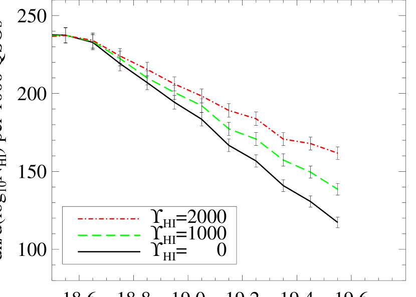
The total magnification experienced by a quasar is the product of the magnification by each absorption system along its line of sight. Thus ${\rm N}^{T}_{\rm HI}$ has a stronger correlation with magnification than the column densities of individual absorption systems. Another advantage of the ${\rm N}^{T}_{\rm HI}$ quantity is that its measurement does not require assumptions on cosmology. Figure 5 shows $P({\rm N}^{T}_{\rm HI})$ for three values of $\Upsilon_{\rm HI}$. There is a dramatic dependence on $\Upsilon_{\rm HI}$ in the distribution $P({\rm N}^{T}_{\rm HI})$ for higher total column densities. This should be compared to Fig. 2 where the effect of lensing was much less evident.

4.2.2 Rejection of the null hypothesis

We first examine the rejection levels of the null hypothesis that the sample under consideration is not magnified at all. Under this assumption any deviation from the expected $P({\rm N_{HI}},z)$ is purely because of Poisson errors due to a finite sample and observational errors. As discussed above the relevant distribution function to maximize the lensing detection is $P({\rm N}^{T}_{\rm HI})$ rather than $P({\rm N_{HI}},z)$. The equivalent projection along the $z$ axis, $P_{{\rm N_{HI}}}(z)=\int{\rm d}{\rm N_{HI}}P({\rm N_{HI}},z)$ can in principle also be used, as we demonstrated in Fig. 2. Let us first phrase the statistics we use in the conventional $\chi^{2}$ terms and then modify it to get a statistic which is more appropriate for the problem under consideration.

For a sample of $n_{\rm QSO}$ quasars, let $n^{\rm model}_{j}({\rm N}^{T}_{\rm HI})$ be the number of expected absorber in bin $j$ spanning the range $[{\rm N}^{T}_{\rm HI},{\rm N}^{T}_{\rm HI}+\Delta{\rm N}^{T}_{\rm HI}]$. This number depends, of course, on the redshift distribution of the quasars in the sample. Let $\tilde{n}^{\rm model}_{i}(z)$ be the number of expected absorbers in bin $i$ that spans the redshift range $[z,z+\Delta z]$. If the two observed values of the same quantities are $n^{\rm obs}_{j}({\rm N}^{T}_{\rm HI})$ and $\tilde{n}^{\rm obs}_{i}(z)$ we can construct the two $\chi^{2}$ functions

$$\chi^{2}_{1} = \sum_{j}{{\left[(n^{\rm model}_{j}({\rm N}^{T}_{\rm HI})-n^{\rm obs}_{j}({\rm N}^{T}_{\rm HI})\right]^{2}}\over{\epsilon_{{\rm poisson},j}^{2}+\epsilon_{{\rm error},j}^{2}}}$$

$$\chi^{2}_{2} = \sum_{i}{{\left[(n^{\rm model}_{i}(z)-n^{\rm obs}_{i}(z)\right]^{2}}\over{\epsilon_{{\rm poisson},i}^{2}+\epsilon_{{\rm error},j}^{2}}}\,,$$ (13)

where the sums are over the relevant bins. The two error contributions are from the Poisson error due to the finite sample, $\epsilon_{\rm poisson}$ and the propagating error due to the observational uncertainty in $N_{\rm HI}$. The slope in the $P(N_{\rm HI})$ function is affected by a Malmquist-like bias since it is more likely for lower column density systems to “leak” into a bin of higher column density than the other way around. We therefore adopted the following form for the error terms,

$$\epsilon_{{\rm poisson},j}=\left(n^{\rm model}_{j}\right)^{-1/2}$$ (14)

$$\epsilon_{{\rm error},j}={\frac{1}{2}{\delta{\rm N}_{\rm HI}}\over{\Delta{\rm N}^{T}_{\rm HI}}}\left(n^{\rm model}_{j-1}-2n^{\rm model}_{j}+n^{\rm model}_{j+1}\right),$$

where $\delta{\rm N}_{\rm HI}$ is the measurement error in ${\rm N_{HI}}$ ($15\%$). We approximate the Poisson error from the modeled (expected) $n_{j}$ since ultimately we would like to get a probability distribution about the true underlying value of $\Upsilon_{\rm HI}$.

The two functions, $\chi^{2}_{1,2}$ are not independent as written in Eq. (13). If, for instance the total number of observed absorption systems exceeds the expected one, this will affect both the $\chi^{2}$ values. In order to regain the statistical independence, one of the $\chi^{2}$ functions should be renormalized such that the modified function is read

$${\tilde{\chi}}^{2}_{2}={\sum_{i}{\left({{n^{\rm model}_{i}(z)}\over{\sum_{i}n^{\rm model}_{i}(z)}}-{{n^{\rm obs}_{i}(z)}\over{\sum_{i}n^{\rm obs}_{i}(z)}}\right)^{2}}\over{{\tilde{\epsilon}}_{{\rm poisson},i}^{2}+{\tilde{\epsilon}}_{{\rm error},i}^{2}}}\,,$$ (15)

where the original errors, $\epsilon$, are re-scaled accordingly to ${\tilde{\epsilon}}$. The final $\chi^{2}$ function is then expressed as the weighted sum of the two independent functions

$$\chi^{2}={c_{1}\chi^{2}_{1}+c_{2}{\tilde{\chi}}^{2}_{2}}\,;\,\,c_{1}+c_{2}=1\,.$$ (16)

In practice we find that the statistics is dominated by $\chi^{2}_{1}$ and little improvement in the statistical rejection levels or confidence levels is obtained by including ${\tilde{\chi}}^{2}_{2}$. We therefore set $c_{1}=1$ and $c_{2}=0$ for the rest of our analysis. For example, the $\chi^{2}$ statistics allows us to reject the null hypothesis with $n_{\rm QSO}=2\times 10^{4}$ and values of $\Upsilon_{\rm HI}$ of 300, 400 and 500 at the $70\%,82\%$ and $90\%$ confidence levels respectively.

So far we have used standard $\chi^{2}$ statistics. However, in the current case, where we try to detect a non-random process (or to reject the absence thereof) there is a better, more robust way of doing it. Based on Fig. 5 we notice that the high column density end of the ${\rm N}^{T}_{\rm HI}$ distribution can be well fit by a power law. This power-law description is excellent for the non-magnified case, but it provides a reasonable description for the magnified cases as well. A full description of the fit to the non-lensed case is provided by its normalization, $a_{0}$, and its slope $a_{1}$. Recall that since ${\rm N}^{T}_{\rm HI}$ is the (plain, unweighted) sum of the ${\rm N_{HI}}$ of all absorption systems on the line of sight to a quasar, $a_{1}$ is not identical to the slope of ${\rm d}P/{\rm d{\rm N_{HI}}}$ of Eq. (8). The function $P({\rm N}^{T}_{\rm HI})$ is established using $10^{6}$ un-lensed quasars from the mock catalog. From this we determine $n^{\rm model}_{j}({\rm N}^{T}_{\rm HI})$ for a given value of $n_{\rm QSO}$ and bin size. The best fit to the values of $n^{\rm model}_{j}({\rm N}^{T}_{\rm HI})$ and the errors on these values as given by equation (14) provides the value of $(a_{0},a_{1})$.

In the presence of magnification, we expect a coherent deviation from the non-magnified line ($a_{0},a_{1}$) of the ${\rm N}^{T}_{\rm HI}$ distribution. This altered distribution can be fit with the two parameters which describe it best, ($a^{\prime}_{0},a^{\prime}_{1}$), by a standard fitting procedure, which also takes into account an error covariance matrix ${\bf\Delta a}$ which is a function of $n^{\rm model}_{j}({\rm N_{HI}})$ and of the $\epsilon_{j}$s.

Figure 6: Rejection levels for the null hypothesis that the observed distribution of ${\rm N}^{T}_{\rm HI}$ is unbiased by gravitational lensing as a function of the number of quasars in the sample and the value of $\Upsilon_{\rm HI}$. $n_{\rm QSO}$ is the total number of quasar in the sample, but only a subset of these quasars are used in order to calculate the rejection levels. The subset is determined by a cut in ${\rm N}^{T}_{\rm HI}$ so that $19.0<\log{\rm N}^{T}_{\rm HI}<19.7$. This amounts to $10\%$ of the $n_{\rm QSO}$ in the case of no lensing and increases to $12\%$ if $\Upsilon_{\rm HI}$ is 1000.

At this point the new statistic we establish compares two lines; the model line ($a_{0},a_{1}$) and the fit to the observed line ($a^{\prime}_{0},a^{\prime}_{1}$). We use Monte-Carlo runs to map the probability space in the parameters ($a_{0},a_{1}$) of the non-magnified ${\rm N}^{T}_{\rm HI}$ distribution and to evaluate the probability of fitting a line (in log) of normalization $a^{\prime}_{0}$ and slope $a^{\prime}_{1}$ given a random, discrete realization of this distribution with $n_{\rm QSO}$ lines of sight. The outcome is a full map of the distribution ${\rm d}P/({\rm d}a_{0}{\rm d}a_{1})$ which is similar to Eqs. (13) replacing $n^{\rm model}_{j}({\rm N_{HI}})$ by the fit to the modeled ${\rm N}^{T}_{\rm HI}$ and $n^{\rm obs}_{j}({\rm N_{HI}})$ by the fit to the realization of the ${\rm N}^{T}_{\rm HI}$ distribution. Under this change of variables there is no longer summation over bins and the function which effectively replaces $\chi^{2}$ becomes,

$$\psi={|(a_{0},a_{1})-(a^{\prime}_{0},a^{\prime}_{1})|^{2}\over|{\bf\Delta a}|}\,.$$ (17)

For the z distribution this statistic cannot be used because magnification causes an increase of the number of systems in some bins and a decrease in others. Thus a magnified distribution is no longer well fit by a line (in the log). To compare instead an observed $z$ distribution with a non-magnified one, we use the standard Kolmogorov-Smirnov test.

Figure 7: Same as Fig. 6, but rejection levels are drawn based only on quasars with $19.5<\log{\rm N}^{T}_{\rm HI}<19.7$ which corresponds to $2.1\%$ and $2.7\%$ of $n_{\rm QSO}$  for $\Upsilon_{\rm HI}=0$ and $\Upsilon_{\rm HI}=1000$ respectively.

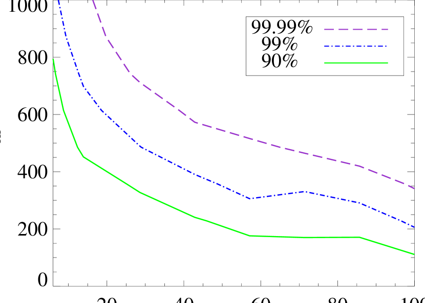
Based on this $\psi$ statistic we can draw rejection levels of the null hypothesis. These are more stringent than those obtained using $\chi^{2}$; for example with a sample of $2\times 10^{4}$ quasars an $\Upsilon_{\rm HI}$ of 600 can be rejected with $99.4\%$ confidence using the $\psi$ statistic, but with only $96\%$ confidence using $\chi^{2}$. Figure 6 shows the rejection levels as function of $n_{\rm QSO}$ and the true modeled value of the constant $\Upsilon_{\rm HI}$. Even though $n_{\rm QSO}$ is of the order $10^{4}-10^{5}$ ($x$ axis), the rejection levels are drawn from a subset of quasars that were selected based on their ${\rm N}^{T}_{\rm HI}$ value. This subset amounts to $10\%$ of the quasars if $19<\log{\rm N}^{T}_{\rm HI}<19.7$ and $\Upsilon_{\rm HI}=0$ and increases to $12\%$ for $\Upsilon_{\rm HI}=1000$. As expected, the rejection confidence increases with increasing $n_{\rm QSO}$ and $\Upsilon_{\rm HI}$. For example, it is enough to have a total sample of $2\times 10^{4}$ quasars in order to reject the null hypothesis by more than $99\%$ for a true $\Upsilon_{\rm HI}$ value of $600$. Recall that only about one tenth of this sample is actually being used in this calculation.

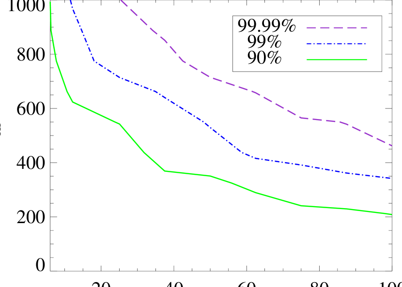
The fraction of the sample that is actually being used can be further reduced by a factor of $4-5$ if a higher lower limit for ${\rm N}^{T}_{\rm HI}$ is adopted. Figure 7 shows the rejection levels if only quasars with $19.5<\log{\rm N}^{T}_{\rm HI}<19.7$ are taken into account. This reduces the sample to $\sim 2.1\%$ and $\sim 2.7\%$ of the size of the original sample for $\Upsilon_{\rm HI}=0$ and $\Upsilon_{\rm HI}=1000$ respectively. However it now takes about $4.5\times 10^{4}$ quasars in the original sample in order to reject the null hypothesis at the $99\%$ confidence level for a true $\Upsilon_{\rm HI}$ value of $600$.

4.2.3 Confidence levels for recovered $\Upsilon_{\rm HI}$

Rejection of the null hypothesis is only the first step in establishing the value of $\Upsilon_{\rm HI}$ and its functional shape. Similarly to the choice of $c_{2}=0$ in the $\chi^{2}$ statistics of the previous section (§4.2.2, Eq. 16), we only consider the change in the number counts in ${\rm N}^{T}_{\rm HI}$ bins since the information in the change of the redshift distribution does not improve the confidence levels by more than a few percent .

To get the best value of $\Upsilon_{\rm HI}$ we de-magnify each quasar in the sample individually, based on the actual absorption systems along its line of sight. The observed flux, $S^{\prime}_{j}$ of a quasar $j$ at $z_{j}$ is shifted to the de-magnified flux, $S_{j}$ by

$$S^{\prime}_{j}\rightarrow S_{j}={S^{\prime}_{j}\over\prod_{i}\mu_{j,i}(z_{j},z_{i},{\rm N_{HI}}^{i};\Upsilon_{\rm HI})}\,,$$ (18)

where $\mu_{j,i}$ is the magnification due to the absorption system $i$ of column density ${\rm N_{HI}}^{i}$ at $z_{i}$ on the line of sight to the quasar, according to Eq. (7). If $S_{j}$ turns out to be lower than the “survey” flux limit, then quasar $j$ along with all its associated absorption systems are removed from the sample. The remaining sample contains $n^{\prime}_{\rm QSO}$$(\leqslant n_{\rm QSO}$) quasars with a set of $n^{\prime}_{\rm QSO}$values of ${\rm N}^{T}_{\rm HI}$. Then in order to account for the dilution of quasars due to solid-angle magnification, we add quasars in the following way. Quasars are drawn randomly from the remaining sample with a probability $1/\mu$ and then added to the sample such that there are duplicates of some of the quasars and their ${\rm N}^{T}_{\rm HI}$ values. These values are fit (in the log) to a linear function characterized by $(a^{\prime}_{0},a^{\prime}_{1})$ and compared to the non-magnified (i.e., the extrapolation from the low ${\rm N}^{T}_{\rm HI}$ range) distribution fit. This is done in the same manner described in §4.2.2. The best $\Upsilon_{\rm HI}$ value is obtained by minimization of the $\psi$ statistic.

Figure 8 shows the success of the recovery of $\Upsilon_{\rm HI}$ values along with its confidence levels. The ratio of the recovered value ($\Upsilon_{\rm HI}^{r}$) and the true pre-assigned value ($\Upsilon_{\rm HI}^{t}$) is shown as a function of $\Upsilon_{\rm HI}^{t}$. Only quasars with $19.0<\log{\rm N}^{T}_{\rm HI}<19.7$ were used to draw the confidence levels. As the total $n_{\rm QSO}$ increases (from the top panel down) the confidence levels of the recovery for a given true $\Upsilon_{\rm HI}^{t}$ value become narrower about this value. Note that the average recovered value is not biased even when the confidence levels are broad.

All quantities are calculated using between $10-20$ Monte-Carlo runs depending on the value of $n_{\rm QSO}$. With a sample of $10^{5}$ quasars it is possible to measure $\Upsilon_{\rm HI}$ to a higher accuracy than $30\%$ of its value if it is greater than 500. This is a remarkable improvement over the current uncertainty of an order of magnitude. The uncertainty in the recovered value of the mass-to-gas ratio does not depend on $\Upsilon_{\rm HI}^{t}$ but only on $n_{\rm QSO}$ (the relative uncertainty as shown in Fig. 8 goes down because $\Upsilon_{\rm HI}^{t}$ increases). The $95\%$ uncertainty in the recovered value of $\Upsilon_{\rm HI}$ is approximately equal to $140\,\sqrt{{10^{5}}\over{n_{\rm QSO}}}$.

Figure 8: The ratio of the recovered ($\Upsilon_{\rm HI}^{r}$) to the true ($\Upsilon_{\rm HI}^{t}$) value of the mass-to-gas ratio and the $95\%$ (shaded region) and $99.7\%$ (dashed line) confidence regions are shown versus $\Upsilon_{\rm HI}^{t}$ for three quasar sample sizes.

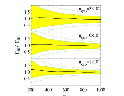
Using only quasars with $19.5<\log{\rm N}^{T}_{\rm HI}<19.7$ out of a sample size of $10^{5}$ quasars has the effect of broadening the confidence levels to the degree of confidence level widths close to the case of $n_{\rm QSO}=6\times 10^{4}$ with $19.0<\log{\rm N}^{T}_{\rm HI}<19.7$.

4.3 Non-constant $\Upsilon_{\rm HI}$

Figure 9: The ratio of the recovered ($\Upsilon_{\rm HI}^{r}$) to the true ($\Upsilon_{\rm HI}^{t}$) value of the mass-to-gas ratio for different mass-to-gas ratio schemes. The top panel is the universal constant scheme explored in §4.2. The middle panel shows the result from a random mass-to-gas ratio with a mean of $\Upsilon_{\rm HI}^{t}$ and a $\sigma_{\Upsilon_{\rm HI}}=\frac{1}{2}\Upsilon_{\rm HI}^{t}$. The bottom panel shows the results from the redshift dependent scheme explained in the text. For all three panels $n_{\rm QSO}=10^{5}$ and quasars with $19.0<\log{\rm N}^{T}_{\rm HI}<19.7$ are used with the $\psi$ statistic. The shaded region and dashed line denote $95\%$ and $99.7\%$ confidence levels respectively.

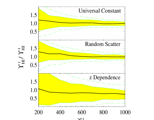
The assumption of a universal mass-to-gas ratio is quite simplistic. We here explore two deviations from this assumption. The first scheme we investigate assumes that $\Upsilon_{\rm HI}$ has a Gaussian distribution with mean $\Upsilon_{\rm HI}$ and standard deviation, $\sigma_{\Upsilon_{\rm HI}}$. The middle panel of Figure 9 shows the recovered value for $\Upsilon_{\rm HI}$ and the confidence levels about it for $\sigma_{\Upsilon_{\rm HI}}=0.5\Upsilon_{\rm HI}^{t}$. Introduction of this significant scatter in the mass-to-gas ratio has a modest effect on the recovery of $\Upsilon_{\rm HI}$. The recovered mean value is slightly higher than $\Upsilon_{\rm HI}^{t}$, but this small bias is less than $50\%$ of the uncertainty of the recovered value of $\Upsilon_{\rm HI}$ even for values of $\sigma_{\Upsilon_{\rm HI}}$ as large as $\Upsilon_{\rm HI}^{t}$. Thus it is only noticeable for small values of $\Upsilon_{\rm HI}^{t}$ as can be seen in Fig. 9. Part of this bias arises because $\Upsilon_{\rm HI}$ must be positive, which skews the Gaussian distribution, thereby increasing the mean value of $\Upsilon_{\rm HI}$. However, there is also the effect that in an observed sample higher values of $\Upsilon_{\rm HI}$ will preferentially be brought into the sample, increasing the mean $\Upsilon_{\rm HI}$ value of observed absorption systems. The scatter in the recovered value shows no noticeable increase for $\sigma_{\Upsilon_{\rm HI}}=0.5\Upsilon_{\rm HI}^{t}$ because the Poisson scatter in the distribution of absorption systems dominates the noise. Thus the statistical nature of the recovery and the large data set being used makes random scatter unimportant in the recovery of $\Upsilon_{\rm HI}$.

The second scheme for the deviation of $\Upsilon_{\rm HI}$ from a universal constant is motivated by the ionization evolution of the Universe. If the ${\rm Y}_{\rm HI}$ parameter of LLS in Eq. (4) is a function of redshift then so is $\Upsilon_{\rm HI}$. For the functional form of ${\rm Y}_{\rm HI}$ we adopt (Haardt & Madau, 1996)

$${\rm Y}_{\rm HI}={\rho_{\rm H}\alpha_{\rm HI}(T)\over\Gamma_{\rm HI}-\rho_{\rm H}\alpha_{\rm HI}(T)}\,$$ (19)

where $\Gamma_{\rm HI}$, the photo-ionization rate per hydrogen atom, is given by

$$A(1+z)^{B}\exp\left[-{(z-z_{c})^{2}\over s}\right]\,,$$ (20)

with the fitting parameters $A=7\times 10^{13}$, $B=0.8$, $s=1.95$, and $z_{c}=2.2$. $\alpha_{\rm HI}$ is assumed to be $2.6\times 10^{-13}$, its value for a $10^{4}\,$K, optically thin gas, with density of $\rho_{\rm H}=4\times 10^{-3}$cm^-3. This roughly corresponds to the virial density and $f_{b}=0.1$. In practice we adjust $A$ so that the maximal $\Upsilon_{\rm HI}$ value we obtain is $3000$.

First, we address the issue of recovering $\Upsilon_{\rm HI}$ under the assumption that it is a universal constant. In this case we will refer to the true value of the mass-to-gas ratio $\Upsilon_{\rm HI}^{t}$ as the average value of $\Upsilon_{\rm HI}$. For the parameters given above the average value is $42\%$ the maximal value.

When $\Upsilon_{\rm HI}$ really does vary with redshift, the bottom panel of Fig. 9 shows the results of the recovery method. The recovered value is about 2/3 the average value which reflects the sensitivity of lensing to redshift as shown in Fig. 4. Also the uncertainty in the recovered value is much wider then in either the universal constant or random scatter schemes.

The second issue of concern is whether we can determine $z_{c}$ in Eq. (20) using our recovery method. First we need to know that $\Upsilon_{\rm HI}$ is a function of $z$ and not a universal constant. This can be done by examining the distribution in redshift of absorption systems with $\log{{\rm N_{HI}}}>19.0$ in the demagnified sample. Figure 10 shows that while the demagnified sample fits the unbiased distribution of ${\rm N_{HI}}$ the $z$ distribution of its absorption systems is markedly different.

Figure 10: The number of absorption systems with $\log{{\rm N_{HI}}}>19.0$ as a function of redshift. The thick solid line is the un-lensed case. The dotted line is the lensed sample magnified by a mass-to-gas ratio that depends on redshift (see text). The dot-dot-dot-dash line is obtained when the sample is erroneously de-magnified by an assumed universal constant value for $\Upsilon_{\rm HI}$. De-magnifying by the correct $z$ dependent scheme results in the dashed line.

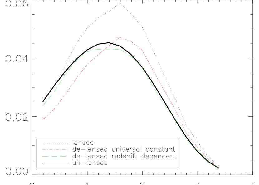
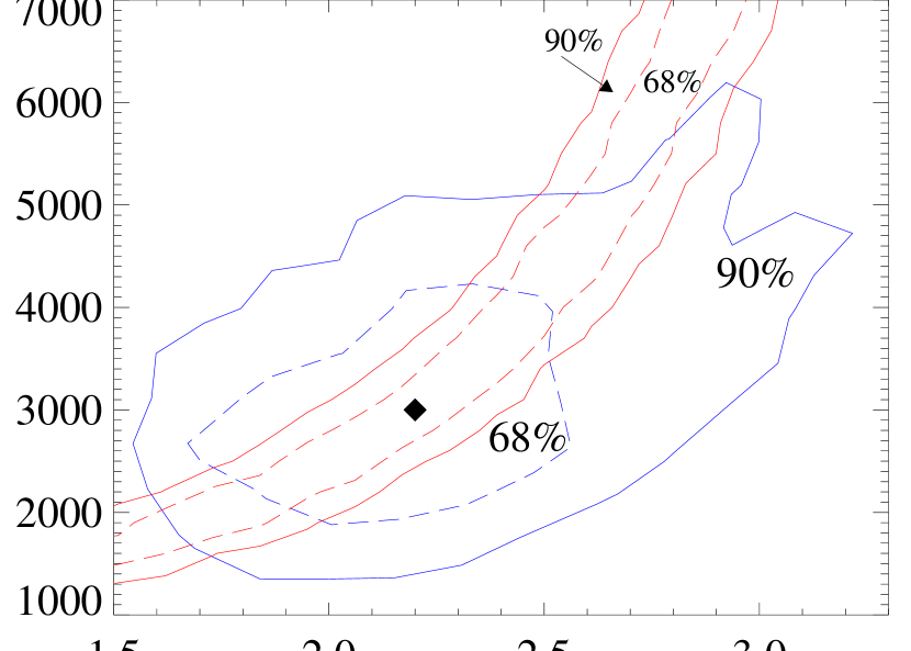
Finding that the assumption of a universal constant $\Upsilon_{\rm HI}$ provides a poor fit to the expected $z$ distribution of absorption systems with $\log{{\rm N_{HI}}}>19.0$, we can try other mass-to-gas schemes. If we assume a function of the form Eq. (20) we can allow $z_{c}$ and the maximum value of $\Upsilon_{\rm HI}$ to vary and compare the resulting de-magnified samples against the expected ${\rm N}^{T}_{\rm HI}$ and $z$ distributions. The results are shown in Figure 11 where the $\psi$ statistic has been used to compare to the ${\rm N}^{T}_{\rm HI}$ while a K-S test is used to determine the probability that the demagnified $z$ distribution is compatible with the expected one. The narrow curve is the constraint from the $\psi$ statistic while the broader, closed region shows the constraints from matching the $z$ distribution. The black diamond shows the true values used in the magnification. Values of $z_{c}$ that are compatible with both tests at better then the $90\%$ level lie between redshifts of 1.5 and 2.9. Thus constraints on the redshift dependence of $\Upsilon_{\rm HI}$ can be placed by considering the $z$ distribution of absorbers in combination with the ${\rm N}^{T}_{\rm HI}$ distribution.

Figure 11: The ability to recover the values of $z_{c}$ and the maximum value of $\Upsilon_{\rm HI}$ using the ${\rm N}^{T}_{\rm HI}$ distribution and the $z$ distribution of absorption systems. The broad, closed region shows the constraints from considering the $z$ distribution and the narrow arc comes from considerations of the ${\rm N}^{T}_{\rm HI}$ distribution. This is done with $n_{\rm QSO}=10^{5}$. Both tests individually allow for a large range in $z_{c}$ but their combination can yield a fairly good measure of these parameters.

4.4 Additional checks for the method

Checks that the signal measured and ascribed to gravitational lensing is really due to gravitational lensing come naturally in our scheme. The first verification is to check that with the recovered value of $\Upsilon_{\rm HI}$ the demagnified sample is in all ways unbiased. The second is to break the observed sample into a part favorable to being lensed and an unfavorable part and then perform the above procedure comparing these two parts.

The correct value of $\Upsilon_{\rm HI}$ should not only bring the distribution of ${\rm N}^{T}_{\rm HI}$ into agreement with what is expected for an un-lensed population, but also the flux function of these demagnified quasars and the redshift distribution of their absorption systems should be in agreement with those quasars that are not significantly lensed. The ability of one value of $\Upsilon_{\rm HI}$ to bring the quasar sample into agreement with these three independent distributions seems quite unlikely if the measured difference in ${\rm N}^{T}_{\rm HI}$ was due to some other effect than lensing. If the $z$ distribution does not match the un-lensed one this does not rule out lensing, it simply rules out the dependence of $\Upsilon_{\rm HI}$ on redshift that we have assumed. A different dependence that is compatible with the three distributions must then be found as has been demonstrated above.

A second check is to divide the sample into those absorber-quasar pairs that are favorable and unfavorable to lensing. Equation 3 shows that lenses of the same mass with redshifts near the redshift of the quasar produce less magnification. Thus separating the sample by this criterion creates a subsample that is in every way identical to the total sample except for this one relationship that should only be relevant to gravitational lensing. The ${\rm N}^{T}_{\rm HI}$ distributions of the two samples can be compared and $\Upsilon_{\rm HI}$ recovered in exactly the same method as explained above. The advantage of this test is that it can be made solely with the data at hand with no need to extrapolate $P({\rm N_{HI}},z)$ from lower column densities; however, because one divides the observed sample into two parts the signal will be reduced. Thus our preference is to assume that we can extrapolate $P({\rm N_{HI}},z)$, and then perform the separation of the sample as an additional check that our assumption is correct. In practice one would first want to validate the assumption that $P({\rm N_{HI}},z)$ can be extrapolated to higher column densities by checking that those systems unfavorable to lensing are consistent with the lower column density $P({\rm N_{HI}},z)$.

5 Observational procedure, metal lines, and dust

The basis of any future large quasar study will be based on the five band photometry of $10^{6}$ quasars and spectra of $10^{5}$ quasars obtained by the SDSS . The Sloan spectra will identify ${\rm Ly-}\alpha~{}$, MgII and CIV lines in the redshift ranges, $2.3<z<6.4$, $0.5<z<2.2$, and $1.6<z<4.8$, respectively.

The detection of ${\rm Ly-}\alpha~{}$from the ground is restricted to $z>2$ so only about $15\%$ of the absorption systems we have been considering in §4 will be detected in ${\rm Ly-}\alpha~{}$in the Sloan data. Furthermore these systems will be less favorable to lensing because of the proximity in redshift of the quasar and the absorber. However, as shown in Fig. 6, if the true mass-to-gas ratio exceeds 800 then with only 5000 quasars it is possible to reject $\Upsilon_{\rm HI}=0$ (no lensing) at the $90\%$ confidence level. So it is possible that a lensing signal may be detected with just the LLS identified in the Sloan survey.

MgII, CIV and other metal lines are detectable over a wide range of redshifts from the ground and thus from the Sloan data alone values for $\Upsilon_{\rm MgII}$ and $\Upsilon_{\rm CIV}$ can be determined. While the theoretical interpretation of these values is more uncertain than $\Upsilon_{\rm HI}$ because of the added complication of metallicity of the gas, nonetheless metal lines can establish that there is lensing by absorption systems. The mass-to-metal-line ratios of different elements can be used to study the enrichment history of LLS. Using correlations between metal line and ${\rm Ly-}\alpha~{}$column density, $\Upsilon_{\rm HI}$ can also be inferred, though with a bigger scatter.

The optimal sample consists of LLS below redshift 2. The Cosmic Origins Spectrograph (COS) to be installed on the Hubble Space telescope and the Galaxy Evolution Explorer (GALEX) will both be able to detect ${\rm Ly-}\alpha~{}$in the ultraviolet starting in 2003. Of course these missions will not be able to get spectra for $10^{5}$ quasars, but as we have described in §4 we only use the $10-12\%$ of quasars with $\log{\rm N}^{T}_{\rm HI}>19.0$ in measuring the lensing signal and recovering $\Upsilon_{\rm HI}$. Thus if the quasars likely to cross this threshold can be identified from their MgII and/or CIV features in a manner identical to that already done when looking for DLAS (Rao & Turnshek, 2000) it only requires $\approx 10^{4}$ spectra to measure ${\rm N_{HI}}$ in the relevant systems. Since GALEX intends to get spectra for $10^{4}$ quasars it is even feasible that almost the entire Sloan sample can be used in measuring the value of $\Upsilon_{\rm HI}$. Because the method of targeting MgII absorbers is the most effective way to detect DLAS with $z<2$, it is likely that a significant fraction of telescope time will be spent on such an endeavor. About $5-10\%$ of all quasars are expected to have at least one absorption system that is above our upper bound on ${\rm N_{HI}}$ ($5\times 10^{19}{\rm{cm}^{-2}}$) and therefore would not be included in the lensing analysis. Of MgII absorbers $\approx 50\%$ are above this upper bound but the rest will be exactly the higher column density LLS that are needed for the lensing analysis. Thus the prospects of having UV spectra for a large number of quasars with $19.0<\log{\rm N}^{T}_{\rm HI}<19.7$ is reasonably good.

One possible impediment to the method we have described in this paper would be the presence of dust in LLS. Metallicity is usually believed to be connected with the dust content in galactic systems. If in spite of their high ionization states, the LLS do contain dust, then dust absorption may be proportional to ${\rm N_{HI}}$ and may act as a counter effect to the gravitational magnification. A straightforward way to probe whether absorption by dust is important would be to apply the recovery method from photometry at different band filters. Similar values for $\Upsilon_{\rm HI}$ from analyses in different bands should verify the irrelevance of dust reddening. If, however, a filter dependent result is obtained for $\Upsilon_{\rm HI}$ values, this might be an extension of the method which would constrain the dust content in LLS.

6 Conclusions

We have introduced a new statistical method to recover the mass to neutral hydrogen ratio in Lyman limit systems. The method makes use of the connection between the measured column density of individual absorption systems and their contribution to the magnification of their background quasars.

The main effect of the gravitational magnification is the change of slope at the high column density end of the column density distribution function. This can be also seen as a shift in the quasar luminosity function, a shift which depends on column densities. Accompanied effects include a distortion of the redshift distribution for the LLS and a small shift in the quasars redshift distribution for quasars with high column density of total absorption.

The relevant variable for these effects is the total column density in LLS along the line of sight to a quasar. We have simulated in detail the quasar population along with their associated LLS. We have mimicked the observational procedure and demonstrated the ability to recover the right value of the mass to neutral gas ratio, $\Upsilon_{\rm HI}$. If $\Upsilon_{\rm HI}$ is a universal constant in these systems then the $95\%$ confidence level of the recovered $\Upsilon_{\rm HI}$ value is given by $\pm 140\left(\sqrt{{10^{5}}\over{{n_{\rm QSO}}}}\right)$ for a sample size in the range $10^{4}<n_{\rm QSO}<10^{5}$, independent of the value of $\Upsilon_{\rm HI}^{t}$! For a stochastic $\Upsilon_{\rm HI}$ with a Gaussian distribution with standard deviation $\sigma_{\Upsilon_{\rm HI}}$, the $95\%$ confidence levels increase only slightly because the large number of quasars diminishes the effects of stochastic processes. A small bias is also introduced because observed higher values of $\Upsilon_{\rm HI}$ are preferentially brought into the sample and because the mean of an unbiased sample is also slightly higher since $\Upsilon_{\rm HI}$ is always positive. However this bias is relatively small; for the large scatter of $\sigma_{\Upsilon_{\rm HI}}=\Upsilon_{\rm HI}$ the bias is only half as large as the $95\%$ confidence level.

A redshift dependence of the $\Upsilon_{\rm HI}$ value due, e.g., to evolution in the ionization state of the LLS can be recovered to a certain extent by assuming the functional form of the dependence and deriving the free parameters of that form. For a reasonable example of a redshift dependent model (Haardt & Madau, 1996), the maximum ionization redshift can be recovered with an accuracy of $\pm 0.7$ These scaling relations for the recovery ability are all achievable in light of the upcoming quasars survey of the SDSS. Follow up observations from space should then be undertaken in order to fill in the low redshift range of LLS, unaccessible from ground.

So far the mass to neutral gas ratio in LLS is unknown to more than an order of magnitude. The method we presented here enables, for the first time, to constrain this value tightly, hopefully leading to a better understanding of the relation between gas and dark matter in the universe.

References

- Abel & Mo (1998) Abel, T. & Mo, H. J. 1998, ApJ, 494, L151
- Bahcall & Spitzer (1969) Bahcall, J. N. & Spitzer, L. J. 1969, ApJ, 156, L63
- Bartelmann & Loeb (1996) Bartelmann, M. & Loeb, A. 1996, ApJ, 457, 529
- Bartelmann & Schneider (2000) Bartelmann, M. & Schneider, P. 2000, Phys. Rep., in press
- Boyle et al. (1988) Boyle, B. J., Shanks, T., & Peterson, B. A. 1988, MNRAS, 235, 935
- Boyle et al. (2001) Boyle, B. J., Shanks, T. C. S. M., Smith, R. J., Miller, L., Loaring, N., & Heymans, C. 2001, MNRAS, accepted, astro-ph/0005368
- Churchill et al. (1996) Churchill, C. W., Steidel, C. C., & Vogt, S. S. 1996, ApJ, 471, 164
- Croft et al. (1998) Croft, R. A. C., Weinberg, D. H., Katz, N., & Hernquist, L. 1998, ApJ, 495, 44
- Dekel & Lahav (1999) Dekel, A. & Lahav, O. 1999, ApJ, 520, 24
- Gardner et al. (1999) Gardner, J. P., Katz, N., Weinberg, D. H., & Hernquist, L. 1999, astro-ph/9911343
- Haardt & Madau (1996) Haardt, F. & Madau, P. 1996, ApJ, 461, 20
- Hamana et al. (2000) Hamana, T., Martel, H., & Futamase, T. 2000, ApJ, 529, 56
- Hartwick & Schade (1990) Hartwick, F. D. A. & Schade, D. 1990, ARA&A, 28, 437
- Hernquist et al. (1996) Hernquist, L., Katz, N., Weinberg, D. H., & Miralda-Escude, J. 1996, ApJ, 457, L51
- Hu et al. (1995) Hu, E. M., Kim, T., Cowie, L. L., Songaila, A., & Rauch, M. 1995, AJ, 110, 1526
- Kaiser & Squires (1993) Kaiser, N. & Squires, G. 1993, ApJ, 404, 441
- Katz et al. (1996) Katz, N., Weinberg, D. H., Hernquist, L., & Miralda-Escude, J. 1996, ApJ, 457, L57
- Kim et al. (1997) Kim, T., Hu, E. M., Cowie, L. L., & Songaila, A. 1997, AJ, 114, 1
- Kirkman & Tytler (1997) Kirkman, D. & Tytler, D. 1997, ApJ, 484, 672
- Kirkman et al. (2000) Kirkman, D., Tytler, D., Burles, S., Lubin, D., & O’Meara, J. M. 2000, ApJ, 529, 655
- Lu et al. (1996) Lu, L., Sargent, W. L. W., Womble, D. S., & Takada-Hidai, M. 1996, ApJ, 472, 509
- Maller et al. (2001) Maller, A. H., Prochaska, J. X., Somerville, R. S., & Primack, J. R. 2001, MNRAS, submitted
- Mo & Miralda-Escude (1996) Mo, H. J. & Miralda-Escude, J. 1996, ApJ, 469, 589
- Narayan & Bartelmann (1999) Narayan, R. & Bartelmann, M. 1999, in Formation of Structure in the Universe, ed. A. Dekel & J. P. Ostriker (Cambridge: University Press), 360–432
- Pei (1995a) Pei, Y. C. 1995a, ApJ, 440, 485
- Pei (1995b) —. 1995b, ApJ, 438, 623
- Petitjean (1998) Petitjean, P. 1998, in Formation and Evolution of galaxies, ed. O. L. Fevre & S. Charlot, Les Houches (Springer-Verlag), astro-ph/9810418
- Porciani & Madau (2000) Porciani, C. & Madau, P. 2000, ApJ, 532, 679
- Press & Rybicki (1993) Press, W. H. & Rybicki, G. B. 1993, ApJ, 418, 585
- Prochaska (1999) Prochaska, J. X. 1999, ApJ, 511, L71
- Prochaska & Wolfe (1996) Prochaska, J. X. & Wolfe, A. M. 1996, ApJ, 470, 403
- Rao & Turnshek (2000) Rao, S. M. & Turnshek, D. A. 2000, ApJS, accepted
- Rauch (1998) Rauch, M. 1998, ARA&A, 36, 267
- Rauch et al. (1997) Rauch, M., Haehnelt, M. G., & Steinmetz, M. 1997, ApJ, 481, 601
- Schneider et al. (1992) Schneider, P., Ehlers, J., & Falco, E. E. 1992, Gravitational Lenses (Berlin: Springer-Verlag)
- Smette (1995) Smette, A. 1995, in QSO Absrobtion Lines, ed. G. Meylan (New York: Springer), 275
- Smette et al. (1997) Smette, A., Claeskens, J. F., & Surdej, J. 1997, New Astronomy, 2, 53
- Storrie-Lombardi et al. (1994) Storrie-Lombardi, L. J., McMahon, R. G., Irwin, M. J., & Hazard, C. 1994, ApJ, 427, L13
- Tytler (1987) Tytler, D. 1987, ApJ, 321, 49
- vanden Berk et al. (1996) vanden Berk, D. E., Quashnock, J. M., York, D. G., & Yanny, B. 1996, ApJ, 469, 78
- Wambsganss et al. (1997) Wambsganss, J., Cen, R., Xu, G., & Ostriker, J. P. 1997, ApJ, 475, L81
- Warren et al. (1994) Warren, S. J., Hewett, P. C., & Osmer, P. S. 1994, ApJ, 421, 412
- Wolfe et al. (1986) Wolfe, A. M., Turnshek, D. A., Smith, H. E., & Cohen, R. D. 1986, ApJS, 61, 249
- Zwaan et al. (1997) Zwaan, M. A., Briggs, F. H., Sprayberry, D., & Sorar, E. 1997, ApJ, 490, 173