Chandra X-ray observations of the 3C295 cluster core

Abstract

We examine the properties of the X-ray gas in the central regions of the distant ($z=0.46$), X-ray luminous cluster of galaxies surrounding the powerful radio source 3C295, using observations made with the Chandra Observatory. Between radii of $50-500$ kpc, the cluster gas is approximately isothermal with an emission-weighted temperature, $kT\sim 5$ keV. Within the central 50 kpc radius this value drops to $kT\sim 3.7$ keV. The spectral and imaging Chandra data indicate the presence of a cooling flow within the central 50 kpc radius of the cluster, with a mass deposition rate of approximately 280 $\hbox{$\rm\thinspace M_{\odot}$}{\rm\thinspace yr}^{-1}\,$. We estimate an age for the cooling flow of $1-2$ Gyr, which is approximately one thousand times older than the central radio source. We find no evidence in the X-ray spectra or images for significant heating of the X-ray gas by the radio source. We report the detection of an edge-like absorption feature in the spectrum for the central 50 kpc region, which may be due to oxygen-enriched dust grains. The implied mass in metals seen in absorption could have been accumulated by the cooling flow over its lifetime. Combining the results on the X-ray gas density profile with radio measurements of the Faraday rotation measure in 3C295, we estimate the magnetic field strength in the region of the cluster core to be $B\sim 12\mu$G.

1 Introduction

X-ray observations of clusters of galaxies show that in the central regions of many clusters the cooling time of the intracluster gas is significantly less than a Hubble time (e.g. White, Jones & Forman 1997; Peres et al. 1998). This cooling is thought to lead to a slow net inflow of material towards the cluster centre; a process known as a cooling flow (see Fabian 1994 for a review). X-ray imaging data show that the gas typically ‘cools out’ and is deposited throughout the central few tens to hundreds of kpc in clusters, with ${\dot{M}}(r)\mathrel{\hbox to0.0pt{\lower 3.0pt\hbox{$\sim$}\hss}\raise 2.0pt\hbox{$\propto$}}r$, where ${\dot{M}}(r)$ is the integrated mass deposition rate within radius $r$ (e.g. Thomas, Fabian & Nulsen 1987). Spatially resolved X-ray spectroscopy of nearby clusters with ROSAT and ASCA has confirmed the presence of distributed, relatively cool gas in cooling flows, with spatial distributions and luminosities in good agreement with the predictions from the imaging data and cooling flow models (e.g. Allen & Fabian 1997; Allen et al. 2000).

In this paper we present Chandra (Weisskopf et al. 2000) X-ray observations of the central region of the distant ($z=0.4605$), optically rich (Dressler & Gunn 1992), X-ray luminous (Henry & Henriksen 1986) cluster of galaxies surrounding the powerful radio source 3C295. Previous X-ray imaging studies of the cluster with the Einstein Observatory and ROSAT have suggested that the cluster contains a strong cooling flow in the region surrounding its central radio source (Henry & Henriksen 1986; White et al. 1997; Neumann 1999). Here we present the first spatially resolved X-ray spectroscopy of the cluster which support this hypothesis. We estimate the age of the cooling flow using the Chandra data and show that it is approximately one thousand times older than the central radio source.

Harris et al. (2000) have reported the detection of X-ray emission from the radio hot-spots in 3C295, using the same Chandra observations discussed here, which they associate with synchrotron self-Compton emission. We here extend the combined radio/X-ray analysis and estimate the magnetic field strength in the cluster core.

The cosmological parameters $H_{0}$=50 $\hbox{${\rm\thinspace km}{\rm\thinspace s}^{-1}\,$}{\rm\thinspace Mpc}^{-1}$, $\Omega=1$ and $\Lambda=0$ are assumed throughout. At the redshift of 3C295 ($z=0.4605$), an angular scale of 1 arcsec corresponds to a physical size of 6.87 kpc.

2 Chandra observations and data reduction

The Chandra observations of 3C295 were made using the Advanced CCD Imaging Spectrometer (ACIS) on 1999 August 30, during the performance verification and calibration phase of the mission. The target was observed in the back-illuminated CCD detectors, close to the nominal aim point for the S3 detector. (The source was positioned close to the node-0/node-1 boundary of the chip). The focal plane temperature at the time of the observations was -100C.

We have used the level-2 events file provided by the standard Chandra pipeline processing and the $CIAO$ software available from the Chandra X-ray Center (CXC; http://asc.harvard.edu/ciao/ for our analysis. Further manual screening based on the instrument light curve was also carried out to remove periods of anomalously high background at the beginning and end of the observation. Only those X-ray events with grade classifications of 0,2,3,4 and 6 were included in our final cleaned data set, which had an exposure time of 17.0ks.

3 Basic imaging analysis

3.1 X-ray and radio morphology

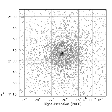
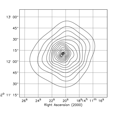
Figure 1: (Left panel) The raw $0.3-7.0$ keV Chandra image of 3C295. The pixel size is 2 detector pixels (0.9838 arcsec). (Right panel) Contour plot of the same region, adaptively smoothed using the code of Ebeling, White & Rangarajan (2001), with a threshold value of $3.5\sigma$. The contours have equal logarithmic spacing.

The raw $0.3-7.0$ keV image for the central $2\times 2$ arcmin² ($0.825\times 0.825$ Mpc²) region of the 3C295 cluster is shown in Fig. 1(a). The pixel size is $0.984\times 0.984$ arcsec², corresponding to $2\times 2$ raw detector pixels. Fig. 1(b) shows an adaptively smoothed contour plot of the same data, using the smoothing algorithm of Ebeling, White & Rangarajan (2001).

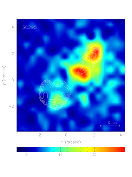
Figure 2: The 8.4 GHz radio image of 3C295 (contours) overlaid on the Chandra image at maximum spatial resolution ($0.492\times 0.492$ arcsec² pixels). The central radio source and hot-spots are clearly detected in X-rays (see also Harris et al. 2000).

Extensive multi-frequency radio observations of 3C295 have been carried out by Perley & Taylor (1991) and Taylor & Perley (1992). These observations reveal a compact (40 kpc diameter) double lobed radio galaxy with prominent steep spectrum hot spots on both sides of a weak flat spectrum core. Fig. 2 shows an 8.4 GHz radio image of the source (contours) overlaid on the $0.3-7.0$ keV Chandra image (in this case shown at maximum spatial resolution with $0.492\times 0.492$ arcsec² pixels). The position for the 8.4 GHz radio core is 14h11m20.53$\pm 0.01$ +52d12m09.69$\pm 0.05$s (J2000.) The Chandra image has been shifted by 0.015 arcsec east and 0.377 arcsec north (these shifts are within the astrometry errors) which provides excellent agreement between the positions of the radio and X-ray core and hot-spots. The central radio source and both radio lobes are clearly detected in X-rays, which Harris et al. (2000) attribute to synchrotron self-Compton emission.

We have searched for the presence of additional patchy substructure in the Chandra images by comparing the data with simple elliptically-symmetric models. The data do not exhibit substructure on scales $>1$ arcsec that is significant at the $>3\sigma$ level, other than that associated with the central radio source. The radio data for the cluster are discussed in more detail in Section 6.

3.2 The surface brightness profile

X-ray emission from the 3C295 cluster is detected out to a radius $r\sim 1$ Mpc (2.4 arcmin) in the Chandra data. Beyond $r\sim 500$ kpc (1.2 arcmin), however, background counts dominate the detected flux. Fig. 3 shows the azimuthally-averaged, $0.3-7.0$ keV surface brightness profile for the central 500 kpc radius. The bin-size is 2 detector pixels (0.984 arcsec). The data have been background subtracted using a rectangular region of size $5\times 1$ arcmin², located $\sim 5.7$ arcmin (2.35 Mpc) from the cluster centre. All point sources, including the central AGN and regions of enhanced emission associated with the radio lobes have been excluded.

Within a radius $r\sim 500$ kpc (excluding the innermost bin associated with the central AGN), the X-ray surface brightness profile can be approximated ($\chi^{2}=101$ for 70 degrees of freedom) by a an isothermal $\beta$-model (e.g. Jones & Forman 1984) of the form $S(r)=S(0)\left[{(1+{r/r_{\rm c})}^{2}}\right]^{1/2-3\beta}$, with a core radius $r_{\rm c}=18.8\pm 1.0$ kpc and a slope parameter $\beta=0.517\pm 0.005$ ($1\sigma$ errors; $\Delta\chi^{2}=1.0$). The best-fitting $\beta$-model is shown overlaid on the surface brightness data in Fig. 3.

3.3 X-ray ‘colour’ profile

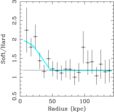
Figure 4: The X-ray colour, defined by the ratio of the counts in the $0.5-1.2$ and $1.3-7.0$ keV bands (soft/hard), as a function of radius. At large radii the ratio is approximately constant and consistent with a temperature $kT=5.0^{+1.3}_{-0.9}$ keV. Within a ‘break’ radius of $53^{+22}_{-19}$ kpc, however, the colour ratio rises sharply indicating the presence of cooler gas. Comparison with the cooling time curve shown in Fig. 13(b) suggests an age for the cooling flow of $1-2$ Gyr. The grey curve shows the predicted colour profile for a cooling flow of age $1.5$ Gyr, assuming that the gas cools from an upper temperature $kT\sim 5$ keV within the central 50 kpc. A metallicity of 0.5 solar and a Galactic column density of $1.3\times 10^{20}$atom cm^-2 are assumed.

In order to investigate radial variations in the temperature of the X-ray gas at high spatial resolution, we have constructed an X-ray colour profile for the central regions of the cluster. Two separate images were created using counts in Pulse Invariant (PI) channels $36-83$ and $84-480$, which cover the observed energy ranges $0.5-1.2$ and $1.2-7.0$ keV (or $0.73-1.75$ and $1.75-10.2$ keV in the rest frame of the source). The soft and hard X-ray images were background subtracted and all significant point sources, including the central AGN and the brightest regions of X-ray emission associated with the radio lobes, were masked out and excluded from the analysis. Azimuthally-averaged surface brightness profiles for the cluster were then constructed in each energy band, centred on the overall peak of the X-ray emission (Section 3.1). The X-ray ‘colour’ profile, formed from the ratio of the surface brightness profiles in the soft and hard bands, is shown in Fig. 4.

Fig. 5 shows the theoretical expectations for the X-ray colour for both isothermal gas and a constant pressure cooling flow, as a function of temperature. (A metallicity of 0.5 solar and a Galactic column density of $1.3\times 10^{20}$atom cm^-2 are assumed.) For the cooling flow predictions, the temperature refers to the upper temperature from which the gas cools). We see that the observed X-ray colour ratio of $1.19\pm 0.12$ in the outer regions of 3C295 (determined from a $\chi^{2}$ fit with a constant model in the $50-140$ kpc range) implies a gas temperature of $5.0^{+1.3}_{-0.9}$ keV (in excellent agreement with the results from the spectral analysis discussed in Section 4.3.1). Within a ‘break’ radius of $53^{+22}_{-19}$ kpc, however, the colour ratio rises sharply, indicating the presence of cooler gas (the $1\sigma$ errors on the break radius are determined from a $\chi^{2}$ fit to the data in Fig. 4 with a broken power-law model). We note that the observed X-ray colour ratio is relatively insensitive to variations in metallicity within the cluster, ranging from 1.19 to 1.17 for isothermal 5 keV gas as the metallicity is varied from $0.0-1.5$ solar.

4 Spatially-resolved spectroscopy

4.1 The regions studied

For our spectral analysis, we have divided the cluster into three annuli, covering the radial ranges $0-50$ kpc (within which the X-ray colour profile shown in Fig. 4  indicates the presence of cooler gas), $50-250$ kpc and $250-500$ kpc. Spectra were extracted from each region in 2048 Pulse Height Analyser (PHA) channels, which were re-grouped to contain a minimum of 20 counts per bin, thereby allowing $\chi^{2}$ statistics to be used. (For the outermost annulus, a grouping of 80 counts per PHA bin was used due to the larger background contribution.) A background spectrum was extracted from a rectangular region, approximately $480\times 140$ arcsec² in size, located well away from the cluster in nodes 2 and 3 of the S3 chip. All significant point sources, including the central AGN, were masked out and excluded from the analysis. In addition, for the central 50kpc region, the X-ray emission associated with the radio lobes (Harris et al. 2000) was excluded using two $2\times 2$ arcsec² square masks. (The X-ray emission from the central AGN and radio lobes are discussed in Section 4.5.)

Separate photon-weighted response matrices and effective area files were constructed for each annular region studied using the calibration and response files appropriate for the focal plane temperature, available from the CXC. Two separate energy ranges were analysed: a conservative $0.5-7.0$ keV range, over which the calibration of the back-illuminated CCDs is currently best understood, and a more extended $0.3-7.0$ keV energy range, which provides extra information on cool emission components and intrinsic absorption in the cluster.

4.2 The spectral models

The analysis of the spectral data has been carried out using the XSPEC software package (version 10.0; Arnaud 1996). The spectra were modeled using the plasma emission code of Kaastra & Mewe (1993; incorporating the Fe L calculations of Liedhal, Osterheld & Goldstein 1995) and the photoelectric absorption models of Balucinska-Church & McCammon (1992). We first examined each annular spectrum using a simple, single-temperature model with the absorbing column density fixed at the nominal Galactic value ($N_{\rm H}=1.33\times 10^{20}$atom cm^-2; Dickey & Lockman 1990). This model is hereafter referred to as model A. The free parameters in model A were the temperature ($kT$) and metallicity ($Z$) of the plasma (measured relative to the solar photospheric values of Anders & Grevesse 1989, with the various elements assumed to be present in their solar ratios) and the emission measure ($K$). We also examined a second single-temperature model (model B) which was identical to model A but with the absorbing column density ($N_{\rm H}$; assumed to act at zero redshift) also included as a free parameter in the fits.

Motivated by the results on the X-ray colour profile shown in Fig. 4 and the results from the deprojection analysis discussed in Section 5.3, we have also examined the spectrum for the central 50 kpc region with a series of more sophisticated, multiphase emission models in which the properties of any cooling flow present can be explicitly accounted for. In the first such model, model C1, the cooling gas was assumed to cool at constant pressure from the ambient cluster temperature, following the prescription of Johnstone et al. (1992). In the second case, model C2, the cooling flow was modeled as an ‘isothermal’ cooling flow, following Nulsen (1998). In both cooling-flow models, the normalization of the cooling-flow component was parameterized in terms of a mass deposition rate, ${\dot{M}}$, which was a free parameter in the fits. Finally, we also examined a more general emission model, model D, in which the cooling gas was modelled by a second, cooler isothermal emission component, with the temperature and normalization of this component included as free fit parameters. Model D provides a more flexible parameterization, with an additional degree of freedom over models C1 and C2, and invariably provides a good match to the more specific cooling-flow models at the spectral resolution and signal-to-noise ratios typical of ACIS observations of distant clusters. However, we found that the ambient cluster temperature was not well constrained with model D, and thus we do not quote explicit results for this model here.

With each of the cooling-flow emission models, we have also examined the effects of including extra absorption, using a variety of different absorption models. In the first case (absorption model i), the only absorption included was that due to cold gas in our Galaxy, with the equivalent column density fixed to the nominal Galactic value (Dickey & Lockman 1990; For a single temperature emission model, this would be identical to spectral model A). In the second model (model ii), the absorption was again assumed to be due to Galactic (zero redshift) cold gas, but with the column density, $N_{\rm H}$, included as a free parameter in the fits. (For a single temperature emission model, this is equivalent to spectral model B.) In the third case (absorption model iii), an intrinsic absorption component with column density, $\Delta N_{\rm H}$, due to cold gas at the redshift of the cluster was introduced. The absorber was assumed to lie in a uniform screen in front of the cooling flow, with the column density included as a free fit parameter. In the fourth case (model iv), the intrinsic absorption was assumed to cover only a fraction, $f$, of the emission from the cooling flow. The fifth and final absorption model (model v) was similar to model (iii) but with the gaseous absorber replaced by an intrinsic absorption edge, with the edge depth, $\tau$, and energy, $E_{\rm edge}$, free parameters in the fits. This general absorption model may be used to approximate the effects of a dusty and/or ionized absorber.

In those cases where the absorption has been quantified in terms of an equivalent hydrogen column density, solar metallicity in the absorbing gas is assumed. We note that in absorption models (iii–v), the absorption acting on the ambient cluster emission was fixed at the nominal Galactic value. However, allowing the Galactic absorption to vary from this value did not significantly improve the fit (at $\geq 95$ per cent confidence) in any case.

4.3 Results from the spectral analysis

The best fit parameter values and 90 per cent ($\Delta\chi^{2}=2.71$) confidence limits determined from the spectral analysis are summarized in Tables $1-3$. For the multiphase analysis of the central 50 kpc region over the restricted $0.5-7.0$ keV band, only the results for absorption models (i) and (ii) are listed, since the other models were poorly constrained. A complete summary of results from the multiphase analysis using the full $0.3-7.0$ keV energy band is provided in Table 3.

4.3.1 Single temperature emission models

Figs. $6-8$ show the Chandra spectra and best-fitting single-temperature models (using model B) for the three annular regions. In all cases, the fits are acceptable in terms of the $\chi^{2}$ values obtained (although for the central 50kpc region, the fits were significantly improved using the multiphase emission plus absorption edge models discussed in Section 4.3.2 below). The results determined in the $0.5-7.0$ and $0.3-7.0$ keV energy ranges show good agreement, arguing against serious calibration problems at low energies in the data. The results for the $50-250$ and $250-500$ kpc annuli both indicate an ambient cluster temperature of $\sim 5$ keV. A joint fit to the data for the two outer annuli with spectral model B over the $0.3-7.0$ keV band gives a mean, ambient cluster temperature, $kT=5.3^{+1.2}_{-0.7}$ keV.

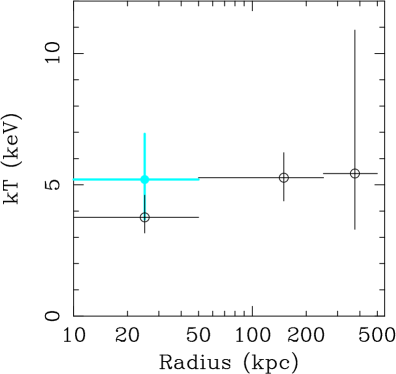
Figure 9: The X-ray gas temperature (and 90 per cent confidence limits) as a function of radius, determined from the $0.3-7.0$ keV data. Open circles show the emission-weighted results determined with the single-temperature model (model B). The ambient temperature in the central 50 kpc region, determined from the multiphase analysis with the effects of the cooling flow and absorption edge accounted for (Section 4.3.2), is shown as the solid grey point.

Within the central 50 kpc region, the results determined with the single temperature models (A and B) indicate a sharp drop in the mean emission-weighted temperature to a value of $\sim 3.7$ keV. (The temperature profile for the X-ray gas determined with spectral model B in the $0.3-7.0$ keV band is shown in Fig. 9.) We find no evidence for intrinsic absorption due to cold gas at any radius using the single temperature models and for all three annuli the best-fit column densities measured with spectral model B are in good agreement with the nominal Galactic value of $1.3\times 10^{20}$atom cm^-2. The results indicate a rather high metallicity, $Z\sim 0.6Z_{\rm\odot}$, across the central 250 kpc of the cluster. (The metallicity at larger radii is not firmly constrained.)

4.3.2 Multiphase emission models

Although the fits to the central 50kpc with spectral models A and B are formally acceptable in terms of their $\chi^{2}$ values, the residuals shown in Fig. 6 indicate a systematic problem at low energies. The data for the outer annuli do not exhibit such poor residuals despite, in the case of the $50-250$ kpc region, having a higher signal-to-noise ratio. We are therefore motivated to examine the improvements in the fits to the spectrum for the central 50 kpc that may be obtained using the more sophisticated, multiphase emission and absorption models described in Section 4.2.

The fits with the multiphase cooling flow models incorporating variable zero-redshift or intrinsic absorption due to cold gas (absorption models (ii) and (iii)) provide only marginal improvements in $\chi^{2}$ with respect to model A(i). A significantly better fit with the cooling flow emission models ($\Delta\chi^{2}\sim 17$) is obtained, however, when we also include an absorption edge (absorption model v), with an intrinsic edge energy, $E_{\rm Edge}\sim 0.6$keV and an optical depth, $\tau\sim 1$. The best-fit model and data, and the residuals to the fit, are shown in Fig. 10. The improvement in the fit at low energies obtained with cooling flow-plus-edge-absorption model may be seen by comparison with Fig. 6.

We note that a single-temperature emission model incorporating an absorption edge (model A(v) in Table 3 ) does not provide as good a fit. Thus, both a multiphase emission model and an edge-like absorption model are favoured by the data for the central 50kpc region.

We adopt the results determined with spectral model C2(v) as our preferred values, since this is the most physically-motivated model. The results determined with model C2 show that the cluster contains a relatively strong cooling flow in its central 50kpc region, with a mass deposition rate of $281^{+85}_{-95}$ $\hbox{$\rm\thinspace M_{\odot}$}{\rm\thinspace yr}^{-1}\,$. The cooling flow accounts for essentially the entire flux from the central 50 kpc, as expected within the context of the ‘isothermal’ cooling flow model, given the results on the probable size of the cooling flow in Section 5.3. The ambient temperature in the central region of the cluster, corrected for the effects of the cooling flow, is $5.20^{+1.74}_{-1.52}$ keV (shown as the filled circle in Fig. 9), in good agreement with the value measured at larger radii. This indicates that the ambient temperature in the cluster remains approximately isothermal within the central 500 kpc. The metallicity within the central 50 kpc measured with model C2(v), $Z=0.47^{+0.35}_{-0.26}Z_{\odot}$, is in reasonable agreement with the result determined with the simple, single temperature models.

Assuming that the absorption edge is due to oxygen, the element with the largest photoelectric absorption cross section ($\sigma\sim 5\times 10^{-19}$cm²) in this region of the X-ray spectrum, the best-fit edge depth of $\tau=1.14^{+0.97}_{-0.41}$ corresponds to an oxygen column density, $\Delta N_{\rm O}=2.3^{+2.0}_{-0.9}\times 10^{18}$atom cm^-2 and/or an equivalent hydrogen column density, $\Delta N_{\rm H}=2.7^{+2.3}_{-1.0}\times 10^{21}$atom cm^-2. (An oxygen number density relative to hydrogen equal to the solar value of $8.51\times 10^{-4}$ is assumed; Anders & Grevesse 1989). The apparent edge energy of $0.57-0.65$ keV is nominally well-matched to the K-absorption edge of partially ionized oxygen, with an ionization state in the range OIII–OV. However, the gain calibration at low energies ($E<0.5$ keV) is presently uncertain (Section 4.7 ) and the apparent edge energy is probably consistent with any ionization state of oxygen from OI to OV. (The photoelectric absorption cross section for oxygen does not vary greatly for any ionization state from OI-OV).

4.4 Spectral deprojection analysis

The results discussed in Section 4.3 are based on the analysis of projected spectra. In order to estimate the effects of projection, we have also carried out a further analysis of the Chandra data using a simple spectral deprojection technique. (A similar method is described by Buote 2000a).

A series of spectra were extracted for the nested set of annuli defined by $r_{1}<r_{2}\ldots<r_{n}$, which were then used to determine the mean, emission-weighted temperatures and densities for the set of spherical shells defined by the same set of radii. The emission from the annulus between $r_{i}$ and $r_{i+1}$ is made up of contributions from the spherical shell between $r_{i}$ and $r_{i+1}$ and all outer shells. We assume that the emission from each spherical shell is isothermal and absorbed by the Galactic column density. Thus, the spectral model for the annulus between $r_{i}$ and $r_{i+1}$ is a weighted sum of $n-i$ absorbed, isothermal models. The fit to the outermost annulus determines the parameters for the outermost spherical shell, which are held fixed in the spectral models for all remaining annuli. The contribution of the outermost shell to each inner shell is determined by purely geometric factors. The fit to the second annulus inward determines the parameters for the second spherical shell, and so forth, working inward. (This parallels the usual image deprojection procedure.) Fitting of the spectral shells was carried out in the $0.5-7.0$ keV band.

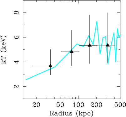
Figure 11: The intrinsic temperature profile determined from the spectral deprojection analysis (Section 4.4; filled triangles) overlaid on the model temperature profile determined using the image deprojection code and best-fit NFW mass model (grey curve). The median model profile determined from 100 monte-carlo simulations is shown).

We have studied six annuli covering the central 2 arcmin of the cluster. No attempt was made to correct for residual emission from the X-ray gas at larger radii since the steeply rising surface brightness profile of the cluster means that only the outer 1 or 2 rings will be significantly affected. (The results for these shells should therefore be viewed with caution, although the temperatures in these regions are poorly determined in any case). The temperature profile determined from the spectral deprojection analysis is shown in Fig. 11. The results are in good agreement with those determined from the projected spectra (Section 4.3.1). We therefore conclude that projection effects do not severely affect the results from the spectral analysis.

4.5 X-ray emission from the central AGN and radio lobes

We have extracted X-ray spectra for the central AGN and the brighter (northwest) of the two radio lobes. In both cases, a square extraction region of size $3\times 3$ pixel² (approximately $1.5\times 1.5$ arcsec²) was used. The local background was determined from a circular region of radius 2.7 arcsec, centred on the AGN, with the emission from the AGN and both radio lobes excluded.

The background-subtracted count rates for both sources are rather low, with a total of 95 and 70 counts for the AGN and northwest lobe, respectively. Fitting a simple power-law model to the spectra, with the column density fixed to the Galactic value of $1.3\times 10^{20}$atom cm^-2, we determine best-fit photon indices of $\Gamma=-0.2\pm 0.4$ for the AGN and $\Gamma=2.7\pm 0.8$ for the X-ray emission associated with the northwest radio lobe. The $0.5-2.0$ and $2.0-10.0$ keV model fluxes are $6.2\pm 2.4\times 10^{-15}$ ${\rm\thinspace erg}{\rm\thinspace cm}^{-2}{\rm\thinspace s}^{-1}\,$($0.5-2.0$ keV) and $2.1\pm 0.7\times 10^{-13}$ ${\rm\thinspace erg}{\rm\thinspace cm}^{-2}{\rm\thinspace s}^{-1}\,$($2.0-10.0$ keV) for the AGN, and $1.2\pm 0.4\times 10^{-14}$ ${\rm\thinspace erg}{\rm\thinspace cm}^{-2}{\rm\thinspace s}^{-1}\,$($0.5-2.0$ keV) and $6^{+9}_{-5}\times 10^{-15}$ ${\rm\thinspace erg}{\rm\thinspace cm}^{-2}{\rm\thinspace s}^{-1}\,$($2.0-10.0$ keV) for the northwest lobe. The very flat slope for the X-ray spectrum associated with the AGN suggests that the emission from the nucleus is heavily obscured and that the observed flux is primarily due to X-ray photons Compton-scattered into our line of sight by cold, optically thick material close to the central X-ray source (e.g. Lightman & White 1988; George & Fabian 1991; Matt, Perola & Piro 1991).

4.6 Comparison with previous results

Our results on the properties of the cluster gas, central AGN and northwest radio lobe are in good agreement with those reported by Harris et al. (2000). These authors measured a mean, emission-weighted temperature of $4.4\pm 0.6$ keV from a fit with spectral model A to the $0.5-7.0$ keV data from within 90 arcsec of the nucleus. A similar, combined fit to the data from all three annuli studied in this paper (which together cover the central 73 arcsec radius) with spectral model A gives $kT=4.61^{+0.55}_{-0.45}$ keV ($0.3-7.0$ keV) or $kT=4.37^{+0.50}_{-0.39}$ keV using the $0.5-7.0$ keV data. (The temperature and metallicity are linked to take the same values in each annulus.) This mean, emission-weighted temperature is lower than the ambient cluster temperature and reflects the presence of cooler gas in the central region of the cluster.

The best-fit ambient cluster temperature of $kT=5.3^{+1.2}_{-0.7}$ keV, determined from a combined analysis of the Chandra data for the $50-500$ kpc region, is slightly cooler than the value of $7.1^{+2.1}_{-1.3}$ keV reported by Mushotzky & Scharf (1997), based on ASCA observations. Our own analysis of the same ASCA Solid-State Imaging Spectrometer (SIS0) data for the central 3.0 arcmin (radius) region of the cluster, using updated calibration files and spectral model B, gives a value $kT=5.0^{+2.4}_{-1.5}$ keV, with a metallicity of $0.36^{+0.39}_{-0.32}Z_{\odot}$ and an absorbing column density $N_{\rm H}=7^{+9}_{-7}\times 10^{20}$ atom cm^-2, in good agreement with the Chandra results. We note that the application of standard screening procedures to the ASCA observation of 3C295 excludes the bulk of the Gas Scintillation Imaging Spectrometer (GIS) data. (We have also excluded the SIS1 data from our analysis, since the cluster centre lies close to the edge of that detector.)

The absorption-corrected bolometric luminosity of the 3C295 cluster ($L_{Bol}=2.3\pm 0.3\times 10^{45}$${\rm\thinspace erg}{\rm\thinspace s}^{-1}\,$) determined from the ASCA data is in good agreement with the value of $2.6^{+0.4}_{-0.2}\times 10^{45}$${\rm\thinspace erg}{\rm\thinspace s}^{-1}\,$ reported by Neumann (1999), based on ROSAT observations. Applying the cooling-flow corrected $kT-L_{\rm Bol}$ relation for cooling-flow clusters determined by Allen & Fabian (1998), we find that such a luminosity typically corresponds to a temperature of $5.5-6.5$ keV, in good agreement with the Chandra results.

4.7 Calibration uncertainties and the apparent absorption edge

The data for the central 50 kpc region of the cluster statistically require the introduction of an absorption edge at high formal significance. The application of an F-test indicates that the improvements obtained with spectral models C1(v) and C2(v), with respect to models C1(i) and C2(i), of $\Delta\chi^{2}\sim 17$ for the addition of two extra fit parameters, are significant at $\gg 99$ per cent confidence. However, especially at this early stage in the Chandra mission, it is important to consider how calibration uncertainties may also affect the results.

The presence of an absorption edge in the data for the central 50 kpc region is supported by the absence of such a feature in the data for the outer annuli. Although the introduction of an absorption edge at an energy of 0.63 keV with an optical depth $\tau<0.6$ is permitted (though not required) by the data for the $50-250$ kpc region, the introduction of an edge with an optical depth $\tau=1.14$ (the best fit value for the central 50 kpc) at this same energy leads to a significant increase in $\chi^{2}$ ($\Delta\chi^{2}=24.1$) with respect to the result obtained for no edge. The presence of an edge with the best-fit parameter values determined for the central 50 kpc region can therefore be ruled out in the $50-250$ kpc data at the $4-5\sigma$ level. The data for the outer, $250-500$ kpc region are less constraining and permit the inclusion of an absorption edge at 0.63 keV with an optical depth $\tau<1$, although the introduction of such an edge provides no improvement in $\chi^{2}$. Thus, the absorption signature appears to be concentrated within the central 50 kpc region of the cluster.

The intrinsic edge energy of $0.63^{+0.03}_{-0.05}$ keV (apparent energy $0.43^{+0.02}_{-0.03}$ keV) determined from the analysis of the PHA data with spectral models C1(v) and C2(v) is inconsistent with the neutral K-edge of oxygen, which should occur at an intrinsic energy of $0.53-0.55$ keV (see discussion in Arnaud & Mushotzky 1998). The solid curve in Fig. 12 shows the relative increase in $\chi^{2}$ with respect to the best fit value determined with spectral model C2(v) as the intrinsic edge energy is varied between values of 0.5 and 0.7 keV. It is crucial to note, however, that the gain calibration for the S3 detector is currently only estimated to be accurate to within $\sim 5$ per cent in the range $0.3-0.5$ keV; N. Schulz, private communication.) To check the low-energy gain calibration, we have searched for fluorescent OI K emission in the background spectrum used in our analysis, which should appear at an energy of $0.525$ keV. We indeed detect such a line at an apparent energy of $0.552^{+0.014}_{-0.017}$ keV (90 per cent confidence limits) which suggests the presence of a gain offset of $5.1^{+1.9}_{-3.2}$ per cent at this energy. Applying such a gain correction to our results, we recover a true, intrinsic edge energy of $0.60^{+0.05}_{-0.06}$ keV, which is consistent with the expected edge energy due to neutral oxygen, or indeed any ionization state of oxygen up to OV. (The maximally gain-corrected results are shown as the dashed curve in Fig. 12.)

We have also repeated our analysis of the properties of the absorption edge in the central 50 kpc region using a spectrum extracted in 1024 Pulse Invariant (PI) detector channels (using a gain file appropriate for the observation date). The PI data were grouped to contain a minimum of 20 counts per analysis bin, in an identical manner to the PHA analysis. The best-fit parameters determined from the PI analysis ($kT=4.54^{+2.07}_{-1.18}$ keV, $Z=0.47^{+0.36}_{-0.27}$ $Z_{\rm odot}$, ${\dot{M}}=266^{+95}_{-106}$ $\hbox{$\rm\thinspace M_{\odot}$}{\rm\thinspace yr}^{-1}\,$, $E_{\rm edge}=0.60^{+0.05}_{-0.05}$ keV and $\tau=1.59^{+1.99}_{-0.69}$, giving $\chi^{2}=33.2$ for 42 degrees of freedom using spectral model C2(v)) are in good overall agreement with those determined from the PHA data, although the best-fit edge energy in the PI case is consistent with the expected value for neutral oxygen. (The constraints on the edge energy determined from the PI data are shown as the dot-dashed curve in Fig. 12.) Taking the PI and PHA analyses together, it is apparent that the results on the edge energy should be viewed with caution at present, but are probably consistent with any ionization state of oxygen from OI-OV.

Significant gain calibration errors appear to be limited to low energies in the S3 detector. Analysing a single PHA spectrum for the entire central 500 kpc region, excluding the emission associated with the central AGN, we detect a clear Fe-K line complex at an energy of $\sim 4.5$ keV, from which we determine a redshift $z=0.461^{+0.019}_{-0.017}$ (90 per cent confidence), in excellent agreement with the optically-determined result.

We note that the results on the absorption edge in the central 50 kpc region are insensitive to the choice of background region used in the analysis and to spatial variations in the spectral response across the field of the S3 detector. The fact that the data for the $50-250$ kpc annulus exclude the presence of an edge with the best-fit parameters determined for the central region, also argues against the absorption edge being due to uncertainties in the quantum efficiency of the detector at low energies.

Finally, we note one further possibility which may affect the observed edge energy, which is resonant scattering of the central AGN continuum by OVII gas in the cooling flow. In principle, this could produce an emission line at an energy of 0.57 keV with a flux of a few $10^{-15}$ ${\rm\thinspace erg}{\rm\thinspace cm}^{-2}{\rm\thinspace s}^{-1}\,$, and lead to an apparent shift in the edge energy from 0.54 keV to higher values.

In summary, the presence of a photoelectric absorption edge is statistically required by the Chandra data for the central 50 kpc region of the 3C295 cluster. The edge is not easily explained as an artefact due to calibration or modeling errors, although the results on the edge energy should be viewed with caution at present. Similar results on the edge energy and depth are determined whether we carry out the analysis in PHA or PI bins. We note that similar systematic residuals at low energies have not, as yet, been seen by us in Chandra data sets for other cluster cooling flows.

5 Image Deprojection analysis

We have carried out a deprojection analysis of the Chandra X-ray images using an extensively updated version of the deprojection code of Fabian et al. (1981; see White, Jones & Forman 1997 for details). For this analysis, we first rebinned the observed surface brightness profile (Fig. 3) into 2 arcsec bins. For the innermost bin, we have corrected for the excluded cluster emission in the region of the central AGN by extrapolating an analytic King law fit to the surface brightness profile in the $1-10$ arcsec range. (We associate a systematic error of 25 per cent with the extrapolated central value.)

5.1 The cluster mass model

The observed surface brightness and deprojected temperature profiles (Figs. 3, 11) may together be used to measure the X-ray gas mass and total mass profiles in the cluster. A variety of simple parameterizations for the total mass distribution were examined, including an isothermal sphere (Equation 4-125 of Binney & Tremaine 1987) and a Navarro, Frenk & White (1997; hereafter NFW) profile. In each case, the best-fit parameter values were determined using a simple iterative technique: given the observed surface brightness distribution and a particular parameterized mass model, the deprojection code is used to predict the temperature profile of the X-ray gas, which is then compared with the observations. (We use the median model temperature profile determined from 100 Monte-Carlo simulations.) The parameters for the mass model are stepped through a regular grid of values to determine the best-fit value (minimum $\chi^{2}$) and confidence limits. Spherical symmetry and hydrostatic equilibrium are assumed throughout.

We find that a good match to the observations can be obtained using an isothermal mass model with a core radius, $r_{\rm c}=60\pm 20$ kpc and a velocity dispersion $\sigma=770\pm 50$ ${\rm\thinspace km}{\rm\thinspace s}^{-1}\,$(90 per cent confidence limits). Alternatively, the temperature and surface brightness data can be well-modelled using an NFW mass model with a scale radius, $r_{\rm s}=0.19^{+0.17}_{-0.08}$ Mpc and a concentration parameter, $c=11.0^{+4.9}_{-3.7}$. The normalization of the NFW mass profile may also be expressed in terms of an equivalent velocity dispersion, $\sigma=\sqrt{50}H_{0}r_{\rm s}c=740^{+190}_{-120}$${\rm\thinspace km}{\rm\thinspace s}^{-1}\,$. The deprojected temperature profile predicted by the best-fitting NFW mass model is shown overlaid on the spectral results in Fig. 11.

Smail et al. (1997) measure a projected mass within a radius of 400 kpc of the centre of the 3C295 cluster from a weak lensing analysis of Hubble Space Telescope images of $4.7\pm 0.8\times 10^{14}$$\rm\thinspace M_{\odot}$. This value is approximately twice as large as the projected mass within the same radius implied by the best-fitting NFW X-ray mass model of $2.1^{+0.8}_{-0.5}\times 10^{14}$$\rm\thinspace M_{\odot}$. (We assume that the X-ray mass model extends to an outer radius of 2 Mpc in our calculation of the projected mass). The discrepancy between the lensing and X-ray results is probably due to the presence of significant substructure along the line of sight to the cluster core, which includes the presence of a foreground cluster at $z\sim 0.26$ (Dressler & Gunn 1992). It remains possible, however, that the mean redshift of the lensed sources might exceed the value of 0.83 assumed in the Smail et al. (1997) study (which would cause the lensing mass to be over-estimated) and/or that the temperature of the X-ray gas might rise significantly beyond the central 250 kpc radius. Our results and conclusions regarding the projected mass within the central 400 kpc region of the cluster are consistent with those of Neumann (1999).

5.2 The X-ray gas properties

The results on the the electron density and cooling time of the X-ray gas from the deprojection analysis, using the best-fitting NFW mass model, are shown in Fig. 13. Within a radius of 500 kpc, the deprojected electron density distribution can be approximated ($\chi^{2}=47.6$ for 34 degrees of freedom) by a $\beta$-model with a core radius $r_{c}=17.8\pm 1.3$ kpc, $\beta=0.515\pm 0.013$, and a central density, $n_{\rm e}(0)=0.16\pm 0.01$ cm^-3 ($1\sigma$ errors), although we caution that the results on the central density are sensitive, at the level of a few tens of per cent, to the manner in which the X-ray emission associated with the radio lobes and central AGN are excluded.

For an assumed Galactic column density of $1.3\times 10^{20}$atom cm^-2, we measure a central cooling time (i.e. the mean cooling time within the central 2 arcsec bin) of $t_{\rm cool}=2.1\pm 0.3\times 10^{8}$ yr, and a cooling radius (at which the cooling time first exceeds a Hubble time) of $r_{\rm cool}=145^{+38}_{-30}$ kpc.

The X-ray gas-to-total mass ratio determined from the deprojection analysis is shown in Fig. 14. At $r=500$ kpc (the outermost radius at which reliable temperature and density data are available) we measure $f_{\rm gas}=13.9^{+3.5}_{-4.6}$ per cent (90 per cent confidence limits).

5.3 The mass deposition rate from the cooling flow

The mass deposition profile from the cooling flow, determined from the image deprojection analysis, is shown in Fig. 15. The mass deposition profile is a parameterization of the luminosity distribution in the cluster core, under the assumption that this emission is due to a steady-state cooling flow (for details of the calculation see e.g. White et al. 1997). Since the presence of cooling gas will tend to enhance the X-ray luminosity of a cluster, the outermost radius at which cooling occurs may also be expected to be associated with a ‘break’ in the X-ray surface brightness profile and, more evidently, the mass deposition profile determined from the deprojection code. We have fitted a broken power-law model to the mass deposition profile for 3C295 over the central 200 kpc radius and find that the data exhibit a break at a radius of $32\pm 5$ kpc, which is consistent with the break radius determined from the fit to the X-ray colour profile in Section 3.3. (The best-fit broken power-law model has been overlaid on the mass deposition profile in Fig. 15.)

The slopes of the mass deposition profile internal and external to the break radius are $1.45\pm 0.25$ and $0.28\pm 0.13$, respectively ($1\sigma$ errors determined from a least-squares fit). Accounting only for absorption due to cold gas with the nominal Galactic column density, we measure an integrated mass deposition rate within the break radius determined from the deprojection analysis of $286^{+12}_{-59}$$\hbox{$\rm\thinspace M_{\odot}$}{\rm\thinspace yr}^{-1}\,$. If we also account for the presence of an absorption edge with the best-fit properties determined with spectral model C2(v), the mass deposition rate within the break radius rises to $316^{+13}_{-65}$$\hbox{$\rm\thinspace M_{\odot}$}{\rm\thinspace yr}^{-1}\,$, in reasonable agreement with the independent spectral result of $281^{+85}_{-95}$$\hbox{$\rm\thinspace M_{\odot}$}{\rm\thinspace yr}^{-1}\,$ (Table 3).

The Chandra result on the mass deposition rate is slightly lower than the value of $410^{+125}_{-130}$$\hbox{$\rm\thinspace M_{\odot}$}{\rm\thinspace yr}^{-1}\,$ reported by White et al. (1997) based on Einstein Observatory High Resolution Imager (HRI) observations, and $400-900$$\hbox{$\rm\thinspace M_{\odot}$}{\rm\thinspace yr}^{-1}\,$ reported by Neumann (1999) using ROSAT HRI data. However, both the White et al. (1997) and Neumann (1999) results were based on calculations which assumed a very old age for the cooling flow of 13 and 10 Gyr, respectively. As we discuss below, the Chandra data suggest that the cooling flow in the 3C295 cluster is much younger than this, with an age of $\sim 1-2$ Gyr.

5.4 The age of the cooling flow

Allen et al. (2000) discuss a number of methods which may be used to estimate the ages of cooling flows. (Such ages are likely to relate to the time intervals since the central regions of clusters were last disrupted by major subcluster merger events.) Essentially, these methods identify the age of a cooling flow with the cooling time of the X-ray gas at the break radius measured in either the X-ray colour or deprojected mass deposition profiles.

Combining the results in Figs. 4 and 13, we see that cooling time of the X-ray gas at the break radius measured in the X-ray colour profile ($53^{+22}_{-19}$ kpc; Section 3.3) lies in the range $1.8^{+1.3}_{-0.9}$ Gyr. (The cooling time at the break radius is determined from a least-squares fit to the cooling time data in Fig. 13(b) between radii of $20-80$ kpc using a power-law model.) If we instead identify the age of the cooling flow with the cooling time at the break radius in the mass deposition profile in Fig. 15 ($32\pm 5$ kpc), we infer an age for the cooling flow of $0.8\pm 0.2$ Gyr. In both cases we assume that no intrinsic absorption acts beyond the outer edge of the cooling flow, which is reasonable if the absorbing matter is accumulated by the flow.

Following Allen & Fabian (1997), we may compare the observed X-ray colour profile to the predictions from the deprojection code for a steady-state cooling flow, assuming an age of 1.5 Gyr. This is shown in Fig. 4. The agreement between the observed and predicted values provides further support for the validity of the cooling-flow model in the central regions of the cluster.

In summary, we see that the two methods provide a consistent result on the age of the cooling flow in 3C295, with a preferred value of $1-2$ Gyr. This value is less than the typical age determined for the sample of nearby cluster cooling flows studied by Allen et al. (2000), although implies a similar formation redshift. It is worth emphasising the remarkable capabilities of Chandra, which allow it to constrain the age of the cooling flow in a cluster at a redshift of $z=0.46$, using only a 17ks exposure. The application of similar techniques to Chandra observations of a large sample of clusters should become possible over the next few years. This will provide significant insight into the evolution of cluster cooling flows and an important new data set for comparison with numerical simulations of cluster formation.

6 Radio properties

6.1 The age of the radio source

Based on synchrotron aging arguments and ram pressure confinement of the hot spots, Perley & Taylor (1991) argue that the central radio source in 3C295 has an age of 10⁶ years. The age of the radio source is therefore $\sim 1000$ times less than the age we derive for the cooling flow. The total luminosity of 3C295 in the radio band is $\sim 10^{45}$ ${\rm\thinspace erg}{\rm\thinspace s}^{-1}\,$. Assuming a radiative efficiency of 10 per cent, the ‘waste’ energy supplied by the radio source into its environs is then on the order of 10⁴⁶ ${\rm\thinspace erg}{\rm\thinspace s}^{-1}\,$, which exceeds the absorption-corrected luminosity of the cluster in X-rays. Thus, if the central radio source were intermittently active on a time scale of $\sim 10^{8}$ years, it could have a significant heating effect on the central X-ray gas. However, the cooling flow in 3C295 appears to have remained relatively undisturbed for a period of $1-2$ Gyr.

6.2 Faraday rotation measure and magnetic fields in the cluster gas

The compact, strong hot-spots in 3C295 have minimum pressures of up to 7.3 $\times$ 10^-8 dyn cm^-2. Our deprojection analysis of the Chandra observations leads to a central pressure approximately three times higher than that estimated from Einstein Observatory observations by Henry & Henriksen (1986). In spite of the upwardly revised estimate of the central X-ray pressure, the radio pressures of the hot spots still exceed the thermal gas pressure at the same radius by a factor of $\sim 100$ and ram pressure confinement of the hot spots is required. The radio lobes, however, have minimum pressures of $10^{-9}$ dyn cm^-2 and may be in equipartition with the X-ray emitting gas. In fact, the high brightness of the lobes in 3C295 may be a consequence of its high-pressure environment. Other examples of luminous radio galaxies embedded in cooling flow clusters are 3C84 in the Perseus cluster, Cygnus-A and Hydra A. Overall there is a trend for cD galaxies in dense X-ray emitting clusters to host moderately strong radio galaxies (e.g. Ledlow & Owen 1995), but most are less luminous than 3C295.

The radio galaxy 3C295 has been known for some time to possess very high Faraday rotation measures (RM; Perley & Taylor 1991), reaching 9000 rad m^-2, whereas typical background radio sources along this line of sight through our Galaxy have RMs of just 20 rad m^-2 (Simard-Normandin, Kronberg, & Button 1981). The most likely origin for the high RMs in 3C295 is a cluster magnetic field. To date, all radio galaxies found at the center of dense X-ray emitting clusters exhibit high RMs, with the RM correlating with the central density excess or cooling flow rate (Taylor, Allen & Fabian 1999; Taylor, Barton & Ge 1994).

Faraday rotation of the radio emission from 3C295 will be produced if magnetic fields are intermixed with the hot X-ray emitting gas that surrounds the radio galaxy. The polarization angle obeys a $\lambda^{2}$ law and the relation between the RM, the gas density $n_{e}$, and the magnetic field along the line of sight, $B_{\|}$, is given by

$$RM=812\int\limits_{0}^{L}n_{\rm e}B_{\|}{\rm d}l~{}{\rm radians~{}m}^{-2}~{},$$ (1)

where $n_{e}$ is the electron density in cm^-3, $B_{\|}$ is in $\mu$Gauss, and $l$ is in kpc. On average, the magnetic field, $B$, will be larger than the parallel component, $B_{\|}$, by $\sqrt{3}$.

If the magnetic field is tangled with cells of uniform size, same strength, and random orientation, then the observed RM along any given line of sight will be generated by a random walk process. The expected distribution is Gaussian with a zero mean, and the dispersion is related to the number of cells along the line of sight. The source will also depolarize if the cell size is smaller than the instrumental resolution.

Perley & Taylor (1991) measured the RM distribution in 3C295 and, assuming a constant density and magnetic field strength over a 100 kpc path, derived a field strength of 30 $\mu$G. Using the density profile derived in Section 5.2, and an analysis of the RM dispersion, we can provide a refined estimate for the magnetic field strength. From the patchy appearance of the Rotation Measure image, Perley & Taylor (1991) estimate a coherence length, $l$, of 0.5 arcsec (3.4 kpc). Using a spherical $\beta$-model for the density distribution, the expected dispersion in the RM for a source at the same distance from us as the cluster center has been evaluated by Felten (1996) to be

$$\sigma_{RM}={{441B_{\|}n_{0}r_{c}^{1/2}l^{1/2}}\over(1+r^{2}/r_{c}^{2})^{(6\beta-1)/4}}\sqrt{\Gamma(3\beta-0.5)\over{\Gamma(3\beta)}},$$ (2)

where $\Gamma$ is the Gamma function. Given the RM dispersion in 3C295 (see Fig.16), computed to be 2900 rad m^-2, we estimate $B_{\|}=7.2\mu$G, implying $B\sim 12\mu$G (after scaling by $\sqrt{3}$). The greatest uncertainty in this calculation stems from the knowledge of the cell size. If the cell size is in the range 10–1 kpc then the corresponding magnetic field strength, $B$, is 7–20 $\mu$G. These values are quite similar to the field strengths of 5–10 $\mu$G found in A119 (Feretti et al. 1999), and 7–14 $\mu$G in the 3C129 cluster (Taylor et al. 2001) by a similar analysis.

7 Discussion

7.1 X-ray absorption by dust grains

The absorption edge detected in the central regions of 3C295 is presumably due to oxygen, the element with the largest absorption cross section in this region of the X-ray spectrum. If we assume that the oxygen was initially contained in gas with approximately solar metallicity, and that this material lay in a uniform screen in front of the X-ray emitting region, we may estimate the corresponding gas mass as

$$M_{\rm abs}\sim 3\times 10^{7}r_{\rm abs}^{2}\Delta N_{\rm H}\hbox{$\rm\thinspace M_{\odot}$},$$ (3)

where $r_{\rm abs}$ is the radial extent of the absorber in kpc and $\Delta N_{\rm H}$ is the equivalent hydrogen column density in units of $10^{21}$ atom cm^-2. For $r_{\rm abs}=50^{+30}_{-20}$ kpc and $\Delta N_{\rm H}=2.7^{+2.3}_{-1.0}\times 10^{21}$atom cm^-2 (Section 4.3.2), we obtain $M_{\rm abs}=2.0^{+7.6}_{-1.5}\times 10^{11}$ $\rm\thinspace M_{\odot}$ (although Allen & Fabian 1997 and Wise & Sarazin 2001 argue that for a geometry in which the absorbing material is distributed throughout the X-ray emitting region, the true mass may be a few times higher.)

This gas mass may be compared to the mass expected to have been accumulated by the cooling flow within the same radius over its lifetime ($\sim 1-2$ Gyr; Section 5.4). If from time $t=0$ to $t=2\times 10^{9}$ yr the integrated mass deposition rate increases approximately linearly with time, then after $t=2\times 10^{9}$ yr, the accumulated mass is ${\dot{M}}t/2\sim 4\times 10^{11}$ $\rm\thinspace M_{\odot}$, in reasonable agreement with the inferred mass of absorbing gas. This suggests that the metals responsible for the X-ray absorption could initially have been associated with the cooled gas deposited by the cooling flow.

A cold gaseous absorption model is not favoured by the Chandra data. The absence of significant absorption below the observed edge energy suggests that relatively little neutral hydrogen and helium are present and that the oxygen is therefore likely either to have been depleted onto dust grains or be in a warm, partially ionized state. (Intrinsic column densities of solar metallicity cold gas $\mathrel{\hbox to0.0pt{\lower 3.0pt\hbox{$\sim$}\hss}\raise 2.0pt\hbox{$>$}}2\times 10^{20}$ atom cm^-2, included in addition to the absorption edge, can be excluded at 90 per cent confidence by the Chandra data.)

The possibility that the X-ray absorption commonly detected in cooling flow clusters may be primarily due to dust grains has been investigated by several authors (Voit & Donahue 1995; Arnaud & Mushotzky 1998; Allen 2000; see also Fabian, Johnstone & Daines 1994). In the case of silicate dust grains, the OI K edge at a rest-frame energy, $E\sim 0.54$keV is expected to be strong, with relatively little absorption at lower energies. Arnaud & Mushotzky (1998) presented Broad Band X-ray Telescope observations of the nearby Perseus cluster and showed that the $0.35-7.0$ keV data require significant excess absorption which is better-explained by a simple oxygen absorption edge (which they associate with dust) than by a cold, gaseous absorption model. The introduction of an OI K edge also typically provides at least as good a description as a cold gaseous absorber for the intrinsic absorption detected in $0.6-10.0$ keV ASCA spectra for cluster cooling flows (e.g. Allen et al. 2000 and references therein; in the ASCA band, the effects of a photoelectric absorption edge at 0.54 keV and a cold, gaseous absorber with approximately solar metallicity are essentially indistinguishable).

Optical and UV spectroscopy of the central $5-20$ kpc regions of cluster cooling flows often reveals large amounts of ongoing star formation (e.g. Johnstone, Fabian & Nulsen 1987; Allen 1995; Cardiel et al. 1995, 1998; McNamara et al. 1996; Voit & Donahue 1997, Crawford et al. 1999; McNamara 1999) and significant intrinsic reddening due to dust (Hu 1992; Allen et al. 1995; Crawford et al. 1999). Infrared (e.g. Allen et al. 2000; Hansen et al. 2000) and sub-mm (Edge et al. 1999) observations also require the presence of significant dust masses in the core regions of at least a few nearby and/or exceptionally massive cooling flows. In general, the data are consistent with dust being a ubiquitous feature of the central regions of cluster cooling flows.

The lifetime of grains of radius $a\mu$m to sputtering in hot gas of density $n$ is $\sim 2\times 10^{6}a/n{\rm\thinspace yr}$ (Draine & Salpeter 1979). In the central 50 kpc of 3C295, $n\sim 5\times 10^{-2}$cm^-3, so that for large dust grains with $a\sim 10\mu$m (which are inferred to have formed and carry most of the iron in e.g. the expanding remnant of SN1987A; Colgan et al. 1984) the sputtering timescale is $\sim 4\times 10^{8}$ yr. However, magnetic shielding in cooled clouds deposited from the cooling flow may allow dust grains to survive for significantly longer (B. Chandran, private communication).

7.2 The feasibility of a warm absorber

The possible presence of warm, partially-ionized, spatially-extended absorbing gas associated with cooling flows in nearby galaxies and galaxy groups has recently been explored by Buote (2000a,b) using ROSAT Position Sensitive Proportional Counter (PSPC) data. Buote (2000a,b) shows that the introduction of a simple photoelectric absorption edge at $E\sim 0.54$ keV in the modeling of the PSPC spectra for the central regions of such systems leads to significant improvements in the goodness of fit, in an analogous manner to the results reported here. The explanation for the origin of the absorption favoured by Buote (2000a,b) is that it is due warm ($T\sim$ a few $10^{5}$K), partially ionized gas. However, the existence of such material with masses, in some cases, exceeding the X-ray emitting gas mass within the same radii by factors of $1-10$ is difficult to understand in terms of its thermal stability and pressure support.

In the case of 3C295, a warm, ionized absorber is consistent with the observed edge energy, which allows for any ionization state of oxygen from OI-OV. However, the cooling rate of such material would be extremely rapid with a cooling time $\sim 100$ yr and an implied luminosity $L_{\rm abs}\sim 3\times 10^{47}{(M_{\rm abs}/10^{12}M_{\odot}}){(T/10^{5}K)}^{-3/2}$ ${\rm\thinspace erg}{\rm\thinspace s}^{-1}\,$, occurring mainly in optical/UV line emission (White et al. 1991; see also Loewenstein & Fabian 1990, Daines, Fabian & Thomas 1994; Pistinner & Sarazin 1994). For $M_{\rm abs}\sim 2\times 10^{11}$$\rm\thinspace M_{\odot}$ and $T\sim 10^{5}$ K, $L_{\rm abs}\sim 6\times 10^{46}$ ${\rm\thinspace erg}{\rm\thinspace s}^{-1}\,$, which significantly exceeds the total X-ray luminosity of the cluster. Although detailed UV observations of 3C295 are not currently available to unambiguously test this hypothesis, it is clear that an enormous heat source would be required to maintain the gas at such temperatures.

One possible mechanism for heating the absorbing matter without significantly heating the surrounding hot, X-ray emitting gas (which has the larger volume filling factor and which shows no obvious evidence for excess heating) is photoionization by UV/X-ray radiation from the central AGN. However, detailed calculations carried out by us using the Cloudy code (Ferland 1996; version 94.00) show that one cannot match the required absorbing column density in ionized Oxygen without greatly exceeding the observed optical line luminosities (Baum & Heckman 1989; Lawrence et al. 1996), other than with highly contrived models (see Appendix A for details).

A further difficulty with the warm absorber scenario in the case of 3C295 is in preventing the warm, absorbing gas clouds from falling rapidly into to the cluster centre. To avoid falling inwards, a warm cloud must have sufficient size such that the drag due to the hot gas is negligible. Minimally, this requires that their terminal velocities exceed the Kepler speed i.e.

$${\rho_{w}\over\rho_{h}}{r\over R}>1,$$ (4)

where $\rho_{w}$ is the density of the warm gas, $\rho_{h}$ the density of the hot gas, $r$ the radius of the warm cloud and $R$ the distance to the cluster centre. Even then, the decay time of a cloud’s orbit due to drag from the hot gas can be short;

$$t_{\rm decay}\sim{\rho_{w}\over\rho_{h}}{r\over R}{R\over v_{K}},$$ (5)

where $v_{K}$ is the Kepler speed, which should exceed the age of the cooling flow. For a Kepler speed of $\sim 1000$ ${\rm\thinspace km}{\rm\thinspace s}^{-1}\,$, an age of $2\times 10^{9}$ yr and $R=50$ kpc, this requires

$${\rho_{w}\over\rho_{h}}{r\over R}>40,$$ (6)

which can be translated into a limit on the mass of a warm cloud of

$${4\pi\over 3}\rho_{w}r^{3}>{4\pi\over 3}\rho_{h}R^{3}40^{3}\left(\rho_{h}\over\rho_{w}\right)^{2}$$ (7)

ie the mass of one warm cloud must exceed the mass of all the hot gas (roughly the total mass of cooled gas) unless $\rho_{w}>250\rho_{h}$. The last condition is barely satisfied if the warm gas is in pressure equilibrium and its temperature is $2\times 10^{5}$ K. A further issue is then whether thermally unstable clouds, which almost certainly fail the first condition above when they are first formed, can aggregate to form such a large cloud on a sufficiently fast timescale. (We note that magnetic fields in the warm gas clouds, if sufficiently strong and stable, may contribute to the pressure support of the clouds and slightly reduce the cooling rate, although the cooling will still be very rapid.) It therefore appears that a warm, partially ionized absorber with $T\sim 10^{5}$ K cannot provide a satisfactory explanation for the X-ray absorption detected in the central regions of 3C295.

7.3 On cooling flow models with a low temperature cut-off

Since this paper was submitted, a series of preprints based on the analysis of XMM-Newton data for the cooling flow clusters Abell 1795 (Tamura et al. 2001), Abell 1835 (Peterson et al. 2001) and Sersic 159-03 (Kaastra et al. 2001) have appeared. These works argue that the XMM-Newton data constrain the mass deposition rates from the cooling flows in these clusters, measured using a constant-pressure model, to be significantly less than the values determined from previous image deprojection studies which assumed ages for the cooling flows of $\sim 13$ Gyr, and studies of the integrated cluster spectra observed with ASCA. A model favoured by these authors is a modified cooling flow model with a low temperature cut-off, $kT_{\rm min}$, below which the gas does not cool. These authors measure values for $kT_{\rm min}$ of $\sim 2.4$ keV (Abell 1795; Tamura et al. 2001), $\sim 2.7$ keV (Abell 1835; Peterson et al. 2001) and $\sim 1.4$ keV (Sersic 159-03; Kaastra et al. 2001), respectively.

We have explored whether a cooling flow model with a low temperature cut-off can also provide a good description of the Chandra data for the 3C 295 cluster. Fitting the $0.3-7.0$ keV spectrum for the central 100 kpc radius with spectral models C1(v) and C2(v) including such a cut-off, we measure $kT_{\rm min}<1.0$ keV (model C1v) and $kT_{\rm min}<0.7$ keV (model C2v) at 90 per cent confidence, respectively (other parameters in good agreement with the values listed in Table 3). Over the restricted $0.5-7.0$ keV range, we measure $kT_{\rm min}<1.2$ keV (model C1v) and $kT_{\rm min}<0.8$ keV (model C2v). Thus, the Chandra data for the central regions of the 3C 295 cluster do not require the introduction of a low temperature cut-off in the cooling flow model and constrain the temperature of any such cut-off to be $kT_{\rm min}\mathrel{\hbox to0.0pt{\lower 3.0pt\hbox{$\sim$}\hss}\raise 2.0pt\hbox{$<$}}1$ keV.

Finally, we note that when comparing results on the properties of cooling flows determined from spatially-resolved spectroscopy with XMM-Newton and Chandra with the findings from previous X-ray missions, it is important to consider the strong assumptions involved in the earlier work. Firstly, the typical ages of cooling flows are likely to be significantly less than the canonical, maximum value of 13 Gyr assumed in most previous X-ray imaging studies (Section 5.4; see also e.g. Schmidt, Allen & Fabian 2001). Thus, the true mass deposition rates from the cooling flows are also likely be lower than the previously-published maximal values. Secondly, as discussed by Allen, Ettori & Fabian (2001), the presence of strong ambient temperature gradients in the centres of (at least some) cooling-flow clusters are likely to have caused the mass deposition rates inferred from previous spectral studies based on the analysis of integrated cluster spectra (which could not resolve spatial variations in the ambient cluster temperature), to have overestimated (e.g. by a factor $\sim 3$ in the case of the massive cluster Abell 2390) the true mass deposition rates from the cooling flows.

8 Conclusions

The main conclusions that can be drawn from this work may be summarized as follows:

(i) The 17ks Chandra ACIS-S observation of the cluster of galaxies surrounding the powerful radio source 3C295 ($z=0.46$) provide firm constraints on the properties of the intracluster gas. Between radii of $50-500$ kpc, the X-ray gas appears approximately isothermal with a mean, emission-weighted temperature $kT=5.3^{+1.2}_{-0.7}$ keV (90 per cent confidence limits). Within the central 50 kpc radius, this value drops to $kT\sim 3.7$ keV. The mean metallicity across the central 250 kpc radius is $Z\sim 0.6$ solar.

(ii) The spectral and imaging Chandra data indicate the presence of a cooling flow within the central 50kpc radius of the cluster, with a mass deposition rate of $\sim 280$ $\hbox{$\rm\thinspace M_{\odot}$}{\rm\thinspace yr}^{-1}\,$. We estimate an age for the cooling flow of $1-2$ Gyr, which is $\sim 1000$ times older than the central radio source. The presence of the cooling flow suggests that the radio source has not significantly heated the surrounding X-ray gas. On larger scales, the X-ray gas appears regular and relaxed.

(iii) The Chandra spectrum for the central 50 kpc region associated with the cooling flow exhibits an edge-like absorption feature which can be interpreted as being due to oxygen-rich dust grains. The implied mass in metals seen in absorption may have been accumulated by the cooling flow over its lifetime.

(iv) Combining the X-ray gas density profile measured with Chandra with radio determinations of the Faraday rotation measure in 3C295, we estimate the magnetic field strength in the region of the cluster core to be $B\sim 12~{}\mu$G.

                 

                          

Figure 3: The background-subtracted, azimuthally-averaged radial surface brightness profile for the central 500 kpc region of the 3C295 cluster in the $0.3-7.0$ keV band. The binsize is 0.984 arcsec (6.76 kpc). All point sources, including the central AGN, and the regions of enhanced emission associated with the radio lobes have been excluded.

       

Figure 5: Theoretical expectations for the X-ray colour ratios of isothermal gas (left panel) and a constant pressure cooling flow (right panel) as a function of temperature. The dotted lines in the left panel show the range of values consistent with the observed colour ratio between radii of $50-140$ kpc in 3C295. In the right panel, the temperature is the upper temperature from which the gas cools. A metallicity of 0.5 solar, an absorbing column density of $1.3\times 10^{20}$atom cm^-2 and a redshift of 0.4605, are assumed.

Figure 6: (Upper panel) Chandra spectrum for the central 50 kpc region of 3C295 in the $0.3-7.0$ keV band with the best-fit single-temperature plasma model (model B) overlaid. (Lower Panel) The residuals to the fit in units of $\chi$.

Figure 7: Chandra spectrum for the $50-250$ kpc annulus with the best-fit single-temperature plasma model (model B) overlaid. Other details as in Fig. 6.

Figure 8: Chandra spectrum for the $250-500$ kpc annulus with the best-fit single-temperature plasma model (model B) overlaid. Other details as in Fig. 6.

Figure 10: Chandra spectrum for the central 50 kpc region of 3C295 in the $0.3-7.0$ keV band with the best-fitting cooling flow model incorporating an intrinsic absorption edge (model C2v) overlaid. Note the improvement to the fit at low energies with respect to Fig. 6.

Figure 12: The increase in $\chi^{2}$ from the best-fit value as the edge energy is varied in spectral model C2(v). The solid curve shows the values determined from the PHA analysis with the nominal gain settings. The dotted curve shows the same results when a gain correction of 7 per cent (the maximum shift consistent with the observed energy of the OI K fluorescent emission line) is applied. The dot-dashed curve shows the results determined from the PI analysis (Section 4.7). The horizontal dashed lines mark the 90 per cent (lower curve) and $3\sigma$ confidence levels.

       

Figure 13: The results on (a) the electron density and (b) the cooling time as a function of radius determined from the X-ray image deprojection analysis using the best-fit NFW mass model. A Galactic column density of $1.3\times 10^{20}$ atom cm^-2 is assumed.

Figure 14: The X-ray gas-to-total mass ratio as a function of radius determined from the deprojection analysis. From top to bottom, the three curves show the 90 per cent confidence upper limit, best-fit value (dotted curve), and 90 per cent confidence lower limit.

Figure 15: The mass deposition profile from the cooling flow in 3C295 determined from the deprojection analysis. A Galactic column density of $1.3\times 10^{20}$atom cm^-2 is assumed. The best fitting broken power-law model is overlaid.

Figure 16: Histogram of the rotation measure for all significant pixels in 3C295 derived from the data of Perley & Taylor (1991).

Table 1: The best-fit parameter values and 90 per cent ($\Delta\chi^{2}=2.71$) confidence limits determined from the spectral analysis of the Chandra data using the single-temperature emission models (models A and B). Temperatures ($kT$) are quoted in keV, metallicities ($Z$) as a fraction of the solar value (Anders & Grevesse 1989) and X-ray absorbing column densities ($N_{\rm H}$) in units of of $10^{20}$ atom cm^-2.

		ENERGY RANGE $0.5-7.0$ keV				ENERGY RANGE $0.3-7.0$ keV
		$0-50$kpc	$50-250$kpc	$250-500$kpc		$0-50$kpc	$50-250$kpc	$250-500$kpc
MODEL A
$kT$		$3.57^{+0.58}_{-0.47}$	$5.02^{+0.80}_{-0.61}$	$6.4^{+4.3}_{-2.2}$		$3.72^{+0.65}_{-0.49}$	$5.22^{+0.85}_{-0.65}$	$6.57^{+3.92}_{-2.08}$
$Z$		$0.59^{+0.39}_{-0.32}$	$0.60^{+0.36}_{-0.31}$	$<1.1$		$0.59^{+0.40}_{-0.34}$	$0.60^{+0.36}_{-0.32}$	$<0.90$
$\chi^{2}$/DOF		35.2/40	87.3/76	8.9/8		48.3/48	110.6/88	10.7/10
MODEL B
$kT$		$3.79^{+0.66}_{-0.67}$	$5.44^{+0.95}_{-0.88}$	$4.7^{+6.2}_{-2.0}$		$3.76^{+0.84}_{-0.59}$	$5.27^{+0.95}_{-0.88}$	$5.43^{+5.46}_{-2.12}$
$Z$		$0.59^{+0.41}_{-0.34}$	$0.59^{+0.32}_{-0.37}$	$<2.1$		$0.60^{+0.42}_{-0.34}$	$0.60^{+0.32}_{-0.37}$	$<0.93$
$N_{\rm H}$		$<3.1$	$<2.1$	$<16.9$		$1.19^{+1.51}_{-1.19}$	$1.23^{+1.13}_{-1.04}$	$2.89^{+4.06}_{-2.89}$
$\chi^{2}$/DOF		34.7/39	86.0/75	8.4/7		48.3/47	110.6/87	10.2/9

Table 2: The best-fit parameter values and 90 per cent confidence limits from the multiphase spectral analysis of the central 50 kpc region using the data in the $0.5-7.0$ keV band. The mass deposition rate from the cooling flow (${\dot{M}}$) is given in units of $\hbox{$\rm\thinspace M_{\odot}$}{\rm\thinspace yr}^{-1}\,$. Other details as in Table 1.

			EMISSION MODEL
ABSORPTION MODEL			C1	C2
	$kT_{1}$		$4.30^{+5.62}_{-0.93}$	$4.18^{+3.10}_{-0.82}$
CASE (i)	$Z$		$0.60^{+0.44}_{-0.35}$	$0.60^{+0.44}_{-0.35}$
GALACTIC ABSORPTION	${\dot{M}}$		$78^{+86}_{-75}$	$77^{+86}_{-74}$
	$\chi^{2}$/DOF		32.3/39	32.3/39
	$kT_{1}$		$6.99^{+3.42}_{-3.42}$	$4.66^{+2.35}_{-1.35}$
CASE (ii)	$Z$		$0.60^{+0.42}_{-0.32}$	$0.58^{+0.45}_{-0.30}$
VARIABLE ABSORPTION	${\dot{M}}$		$317^{+172}_{-208}$	$333^{+182}_{-218}$
BY COLD GAS (z=0)	$N_{\rm H}$		$8.29^{+4.86}_{-4.77}$	$8.51^{+4.94}_{-5.43}$
	$\chi^{2}$/DOF		28.3/38	28.1/38

Table 3: The best-fit parameter values and 90 per cent confidence limits from the multiphase spectral analysis of the central 50 kpc region using the data from the full $0.3-7.0$ keV band. The mass deposition rate from the cooling flow (${\dot{M}}$) is in units of $\hbox{$\rm\thinspace M_{\odot}$}{\rm\thinspace yr}^{-1}\,$. Column densities ($N_{\rm H}$) and intrinsic column densities ($\Delta N_{\rm H}$) are in units of $10^{20}$ atom cm^-2. The absorption edge energy ($E_{\rm edge}$) is in units of keV. Other details as in Table 1. For a complete description of the spectral models see Section 4.2

			EMISSION MODEL
			SINGLE-PHASE	MULTIPHASE
ABSORPTION MODEL			A	C1	C2
	$kT_{1}$		$3.72^{+0.65}_{-0.49}$	$3.99^{+1.67}_{-0.72}$	$3.96^{+1.48}_{-0.69}$
CASE (i)	$Z$		$0.59^{+0.40}_{-0.34}$	$0.61^{+0.43}_{-0.35}$	$0.61^{+0.43}_{-0.35}$
GALACTIC ABSORPTION	${\dot{M}}$		—	$28^{+69}_{-28}$	$28^{+69}_{-28}$
	$\chi^{2}$/DOF		48.3/48	47.9/47	47.9/47
	$kT_{1}$		$3.76^{+0.84}_{-0.59}$	$3.98^{+1.80}_{-0.76}$	$3.94^{+1.53}_{-0.72}$
CASE (ii)	$Z$		$0.60^{+0.42}_{-0.34}$	$0.61^{+0.43}_{-0.35}$	$0.61^{+0.43}_{-0.35}$
VARIABLE ABSORPTION	${\dot{M}}$		—	$34^{+105}_{-34}$	$35^{+104}_{-35}$
BY COLD GAS (z=0)	$N_{\rm H}$		$1.19^{+1.51}_{-1.19}$	$1.56^{+2.09}_{-1.56}$	$1.57^{+2.09}_{-1.57}$
	$\chi^{2}$/DOF		48.3/47	47.9/46	47.9/46
	$kT_{1}$		$3.61^{+0.71}_{-0.54}$	$4.06^{+2.05}_{-0.77}$	$1.97^{+0.85}_{-0.38}$
CASE (iii)	$Z$		$0.57^{+0.40}_{-0.32}$	$0.57^{+0.40}_{-0.31}$	$0.37^{+0.27}_{-0.15}$
INTRINSIC ABSORPTION	${\dot{M}}$		—	$120^{+107}_{-108}$	$1796^{+2067}_{-1375}$
BY COLD GAS ($z=z_{\rm clus}$)	$\Delta N_{\rm H}$		$0.84^{+2.55}_{-0.84}$	$18.0^{+52.7}_{-8.6}$	$584.3^{+310.2}_{-188.8}$
	$\chi^{2}$/DOF		48.0/47	45.1/46	40.5/46
	$kT_{1}$		$2.15^{+0.73}_{-0.45}$	$2.32^{+0.80}_{-0.46}$	$2.04^{+0.78}_{-0.45}$
CASE (iv)	$Z$		$0.41^{+0.25}_{-0.17}$	$0.45^{+0.29}_{-0.18}$	$0.38^{+0.26}_{-0.16}$
PARTIAL COVERING	${\dot{M}}$		—	$3198^{+6289}_{-2604}$	$1652^{+2212}_{-1237}$
BY COLD GAS ($z=z_{\rm clus}$)	$\Delta N_{\rm H}$		$586.2^{+330.2}_{-227.6}$	$780.0^{+449.0}_{-302.7}$	$589.4^{+306.6}_{-195.4}$
	$f$		$0.67^{+0.15}_{-0.28}$	$1.00^{+0.00}_{-0.91}$	$1.00^{+0.00}_{-0.91}$
	$\chi^{2}$/DOF		40.8/46	41.4/45	40.5/45
	$kT_{1}$		$3.37^{+0.57}_{-0.53}$	$7.58^{+2.66}_{-3.40}$	$5.20^{+1.74}_{-1.52}$
CASE (v)	$Z$		$0.53^{+0.34}_{-0.30}$	$0.48^{+0.36}_{-0.26}$	$0.47^{+0.35}_{-0.26}$
SIMPLE EDGE	${\dot{M}}$		—	$272^{+78}_{-68}$	$281^{+85}_{-95}$
($z=z_{\rm clus}$)	$E_{\rm edge}$		$0.61^{+0.05}_{-0.08}$	$0.63^{+0.03}_{-0.05}$	$0.63^{+0.03}_{-0.05}$
	$\tau$		$0.38^{+0.39}_{-0.27}$	$1.15^{+1.52}_{-0.44}$	$1.14^{+0.97}_{-0.41}$
	$\chi^{2}$/DOF		43.3/46	31.0/45	30.8/45

Appendix A Photoionization modeling and the plausibility of a warm absorber

As mentioned in Section 7.2, one possible mechanism for heating relatively cool, X-ray absorbing gas clouds without significantly heating the surrounding hot, X-ray emitting gas (which has the larger volume filling factor and which shows no obvious evidence for excess heating) is photoionization by UV/X-ray radiation from the central AGN. We have used version 94.00 of the Cloudy photoionization code (Ferland 1996) to investigate this possibility. Our modeling uses the TABLE AGN command to specify the continuum shape (in a similar manner to Matthews and Ferland 1987), a pressure of $\sim 10^{7}\hbox{${\rm\thinspace cm}^{-3}{\rm\thinspace K}$}$ (which approximates that in the X-ray emitting gas at a radius of $\sim 10{\rm\thinspace kpc}$ from the nucleus), an abundance set matching that used in the X-ray spectral fitting and a heavy element abundance of 0.5 solar. The irradiated clouds were assumed to be free of grains. We have explored a range of ionizing fluxes and examined the resulting column densities in various oxygen ions and the predicted luminosities in a number of optical/UV emission lines.

We initially ran two models corresponding to total photoionizing luminosities of $3\times 10^{45}\hbox{${\rm\thinspace erg}{\rm\thinspace s}^{-1}\,$}$ (model 1) and $10^{46}\hbox{${\rm\thinspace erg}{\rm\thinspace s}^{-1}\,$}$ (model 2). The predicted column densities in various oxygen ions are shown in Table A1. The column density in ionized oxygen is very small when compared with that inferred from the fits to the X-ray spectra with the absorption edge model ($N_{O}=2.3^{+2.0}_{-0.9}\times 10^{18}\hbox{${\rm\thinspace cm}^{-2}\,$}$). The Cloudy models were terminated arbitrarily when the electron temperature fell to 1000K, where the oxygen is predominantly neutral. In principle, there may be an arbitrary amount of gas colder than this in the Cloudy models, subject to the constraint that it is Jeans stable. However, the X-ray data only allow absorption from a full ISM-like absorber with an equivalent neutral hydrogen column density $\mathrel{\hbox to0.0pt{\lower 3.0pt\hbox{$\sim$}\hss}\raise 2.0pt\hbox{$<$}}4\times 10^{20}\hbox{${\rm\thinspace cm}^{-2}\,$}$ (for half solar metallicity) in addition to the absorption edge, which would imply a maximum extra column density in oxygen of $1.7\times 10^{17}\hbox{${\rm\thinspace cm}^{-2}\,$}$. Adding this to the sum of the oxygen column densities in all ionization states ($1.5\times 10^{17}\hbox{${\rm\thinspace cm}^{-2}\,$}$ from the Cloudy models with an ionizing luminosity of $10^{46}\hbox{${\rm\thinspace erg}{\rm\thinspace s}^{-1}\,$}$) gives a total possible column density of $3.2\times 10^{17}\hbox{${\rm\thinspace cm}^{-2}\,$}$, which is still an order of magnitude short of the required value. We also note that allowing the models to continue to temperatures below 1000K causes a large build up of radiation pressure in excess of the thermal pressure.

Table A2 shows the predicted luminosities in the $H\beta$, [OII]$\lambda\lambda 3727,3729$, [OIII]$\lambda 5007$, Ly$\alpha$ and CIV $\lambda\lambda 1548,1552$ lines. There are no ultraviolet spectral observations of 3C295, but the observed [OIII]$\lambda 5007$ luminosity determined from narrow band imaging is $\sim 2.5\times 10^{42}$ ${\rm\thinspace erg}{\rm\thinspace s}^{-1}\,$(Baum & Heckman 1989). Scaling the optical line fluxes measured by Lawrence et al. (1996) to the total [OIII]$\lambda 5007$ luminosity also implies total [OII]$\lambda\lambda 3727,3729$ and $H\beta$ luminosities of $\sim 4.7\times 10^{42}$ and $6.1\times 10^{41}$ ${\rm\thinspace erg}{\rm\thinspace s}^{-1}\,$, respectively. We therefore see that the optical line luminosities predicted by photoionization models 1 and 2 exceed the observed values by $2-3$ orders of magnitude, ruling out such models. (Similar results can be obtained using the tabulated line emissivities of Pistinner & Sarazin 1994.)

A cooling cloud could, in principle, be at a pressure much lower than that inferred from the X-ray emitting gas if there were substantial magnetic pressure support, or if the cloud were to cool isochorically. To investigate how this might change the column densities in various ionization states of oxygen and the predicted optical emission line luminosities, we have run a series of further photoionization calculations at lower pressures. Constant pressure models with $nT\sim 10^{4}\hbox{${\rm\thinspace cm}^{-3}{\rm\thinspace K}$}$ were found to be dominated by radiation pressure in diffuse emission lines and are probably unstable. We have also examined a constant density model (model 3): setting the hydrogen number density to $0.32\hbox{${\rm\thinspace cm}^{-3}\,$}$ and using an ionizing flux appropriate for a nuclear ionizing luminosity of $3\times 10^{45}\hbox{${\rm\thinspace erg}{\rm\thinspace s}^{-1}\,$}$, we found that the pressure ranged from $nT\sim 1.4\times 10^{5}-3.6\times 10^{3}\hbox{${\rm\thinspace cm}^{-3}{\rm\thinspace K}$}$. For such a model, we obtain a much higher degree of ionization, with the column densities in various ionization states of oxygen given in Table A1. There is a substantial amount of oxygen in the four times ionized state, but even more in the twice ionized state. The total oxygen column density in this model is $8.8\times 10^{18}\hbox{${\rm\thinspace cm}^{-2}\,$}$, and could be higher if the model were allow to proceed to cooler temperatures. Again, however, Table A2 shows that very large $H\beta$, [OIII], Ly$\alpha$ and CIV line luminosities are expected, which greatly exceed the observed line fluxes at optical wavelengths, although the [OII] emission is somewhat reduced due to the smaller amount of singly ionized oxygen. Finally, to reduce the [OIII] emission, we have artificially truncated the ionized cloud at a size of $2.3\times 10^{20}{\rm\thinspace cm}$ (model 4). This reduces the [OIII] emission by more than two orders of magnitude, whilst still maintaining a large ionized oxygen column density ($\sim 7\times 10^{17}\hbox{${\rm\thinspace cm}^{-2}\,$}$). A model intermediate between models 3 and 4 could probably produce a sufficient column density in ionized oxygen without over-predicting the optical [OIII]$\lambda 5007$ emission, but would be extremely contrived and still produce strong CIV $\lambda\lambda 1548,1552$ lines. HST observations of the CIV emission lines in 3C295 would provide a definitive test of such a model.

Table 4: Column densities of oxygen in various ionization states from the Cloudy modeling. Column 2 lists the photoionizing luminosity in units of $10^{45}$${\rm\thinspace erg}{\rm\thinspace s}^{-1}\,$. Columns $3-10$ list the column densities in each ionization state of oxygen in atom cm^-2.

	IONIZING	OXYGEN COLUMN DENSITY
MODEL	LUMINOSITY	$O^{0}$	$O^{+}$	$O^{2+}$	$O^{3+}$	$O^{4+}$	$O^{5+}$	$O^{6+}$	$O^{7+}$	$O^{8+}$
1	3.0	1.8E16	2.7E16	1.3E16	3.3E14	3.8E12	—	—	—	—
2	10.0	1.9E16	4.2E16	8.0E16	6.9E15	2.4E14	1.5E12	—	—	—
3	3.0	3.0E18	1.5E17	4.4E18	5.2E17	5.5E17	1.8E17	2.8E16	8.8E13	—
4	3.0	1.5E08	5.6E12	8.9E15	2.0E17	3.4E17	1.3E17	2.1E16	6.8E13	—

Table 5: The predicted optical/UV line luminosities (in ${\rm\thinspace erg}{\rm\thinspace s}^{-1}\,$) determined from the photoionization modeling using the Cloudy code. The models are the same as in Table  4.

MODEL	H$\beta$	[OIII]	[OII]	Ly$\alpha$	CIV
1	$3.0\times 10^{43}$	$1.4\times 10^{44}$	$2.2\times 10^{44}$	$8.3\times 10^{44}$	$3.3\times 10^{41}$
2	$9.1\times 10^{44}$	$9.3\times 10^{44}$	$4.1\times 10^{44}$	$2.4\times 10^{45}$	$9.6\times 10^{42}$
3	$3.0\times 10^{43}$	$4.3\times 10^{44}$	$8.7\times 10^{42}$	$7.5\times 10^{44}$	$9.1\times 10^{43}$
4	$2.1\times 10^{43}$	$2.1\times 10^{42}$	—	$7.0\times 10^{43}$	$2.1\times 10^{43}$

References

- [1] Allen S.W., 1995, MNRAS, 276, 947
- [2] Allen S.W., 2000, MNRAS, 315, 269
- [3] Allen S.W., Fabian A.C., 1997, MNRAS, 286, 583
- [4] Allen S.W., Fabian A.C., 1998, MNRAS, 297, L57
- [5] Allen S.W., Ettori S., Fabian A.C., 2000, MNRAS, in press (astro-ph/0008517)
- [6] Allen S.W., Fabian A.C., Edge A.C., Böhringer H., White D.A., 1995, MNRAS, 275, 741
- [7] Allen S.W., Fabian A.C., Johnstone R.M., Nulsen P.E.J., Arnaud K.A., 2000, MNRAS, in press (astro-ph/9910188)
- [8] Anders E., Grevesse N., 1989, Geochemica et Cosmochimica Acta 53, 197
- [9] Arnaud K.A., Mushotzky R.F., 1998, ApJ, 501, 119
- [10] Arnaud, K.A., 1996, in Astronomical Data Analysis Software and Systems V, eds. Jacoby G. and Barnes J., ASP Conf. Series volume 101, p17
- [11] Balucinska-Church M., McCammon D., 1992, ApJ, 400, 699
- [12] Baum S.A., Heckman T., 1989, ApJ, 336, 681
- [13] Binney J., Tremaine S., 1987, Galactic Dynamics, Princeton Univ. Press, Princeton
- [14] Buote, D.A., 2000a, ApJL, 532, 113
- [15] Buote, D.A., 2000b, ApJ, in press (astro-ph/0001330)
- [16] Cardiel N., Gorgas J., Aragon-Salamanca A., 1995, MNRAS, 277, 502
- [17] Cardiel N., Gorgas J., Aragon-Salamanca A., 1998, MNRAS, 298, 977
- [18] Colgan S.W., Haas M.R., Erickson E.F., Lord S.D., Hollenbach D.J., 1994, ApJ, 427, 874
- [19] Crawford C.S., Allen S.W., Ebeling H., Edge A.C., Fabian A.C., 1999, MNRAS, 306, 857
- [20] Daines S.J., Fabian A.C., Thomas, P.A., 1994, MNRAS, 268, 1060
- [21] Dickey J.M., Lockman F.J., 1990, ARA&A, 28, 215
- [22] Draine B.T., Salpeter E.E., 1979, ApJ, 231, 77
- [23] Dressler A., Gunn J.E., 1992, ApJS, 78, 1
- [24] Ebeling H., White D.A., Rangarajan F.V.N., 2001, MNRAS, in press
- [25] Edge A.C., Ivison R.J., Smail I., Blain A.W., Kneib J.-P., 1999, MNRAS, 306, 599
- [26] Fabian A.C., 1994, A&AR, 32, 277
- [27] Fabian A.C., Johnstone R.M., Daines S.J., 1994, MNRAS, 271, 737
- [28] Fabian A.C., Hu E.M., Cowie L.L., Grindlay J., 1981, ApJ, 248, 47
- [29] Felten J.E., 1996, in Clusters, Lensing, and the Future of the Universe, eds. Trimble V., Reisenegger A., ASP Conference Series, Vol. 88, p. 271
- [30] Ferland G.J., 1996, ‘Hazy, a Brief Introduction to Cloudy’, University of Kentucky, Department of Physics and Astronomy, Internal Report.
- [31] Feretti L., Dallacaca D., Govoni F., Giovannini G., Taylor G.B., Klein U., 1999, A&A, 344, 472
- [32] George I.M., Fabian A.C., 1991, MNRAS, 249, 352
- [33] Hansen L., Jorgensen H.E., Norgaard-Nielsen H.U., Pedersen K., Goudfrooij P., Linden-Vornle M.J.D., 2000, A&A, 356, 83
- [34] Harris D.E. et al. , 2000, ApJL, 530, 81
- [35] Henry J.P., Henricksen M.J., 1986, ApJ, 301, 689
- [36] Hu E.M., 1992, ApJ, 391, 608
- [37] Johnstone R.M., Fabian A.C., Nulsen P.E.J., 1987, MNRAS, 224, 75
- [38] Johnstone R.M., Fabian A.C., Edge A.C., Thomas P.A., 1992, MNRAS, 255, 431
- [39] Jones C., Forman W., 1984, ApJ, 276, 38
- [40] Kaastra J.S., Mewe R., 1993, Legacy, 3, HEASARC, NASA
- [41] Kaastra J.S., Ferrigno C., Tamura T., Paerels F.B.S., Peterson J.R., Mittaz J.P.D., 2001, A&A, in press (astro-ph/0010423)
- [42] Lawrence C.R., Zucker J.R., Readhead C.S., Unwin S.C., Pearson T.J., Xu W., 1996, ApJS, 107, 541
- [43] Ledlow M., Owen F.N., 1995, AJ, 110, 1959
- [44] Liedahl D.A., Osterheld A.L., Goldstein W.H., 1995, ApJ, 438, L115
- [45] Lightman A.P., White T.R., 1988, ApJ, 335, 57
- [46] Loewenstein M., Fabian A.C., 1990, MNRAS, 242, 120
- [47] Matt G., Perola G.C., Piro L., 1991, A&A, 245, 63
- [48] Matthews W.G., Ferland G.J., 1987, ApJ, 323, 456.
- [49] McNamara B.R., 1999, preprint (astro-ph/9911129)
- [50] McNamara B.R., Jannuzi B.T., Elston R., Sarazin C.L., Wise M., 1996, ApJ, 469, 66
- [51] Mushotzky R.F., Scharf C.A., 1997, ApJL, 482, 13
- [52] Navarro J.F., Frenk C.S., White S.D.M., 1997,ApJ, 490, 493
- [53] Neumann D.M., 1999, ApJ, 520, 87
- [54] Nulsen P.E.J., 1998, MNRAS, 297, 1109
- [55] Peres C.B., Fabian A.C., Edge A.C., Allen S.W., Johnstone R.M., White D.A., 1998, MNRAS, 298, 416
- [56] Perley R.A., Taylor G.B., 1991, AJ, 101, 1623
- [57] Peterson J.R., Paerels F.B.S., Kaastra J.S., Arnaud M., Reiprich T.H., Fabian A.C., Mushotzky R.F., Jernigan J.G., Sakelliou I., 2001, A&A, in press (astro-ph/0010658)
- [58] Pistinner S., Sarazin C.L., 1994, ApJ, 433, 577
- [59] Schmidt R., Allen S.W., Fabian A.C., 2001, MNRAS, submitted
- [60] Simard-Normandin M., Kronberg P.P., Button S., 1981, ApJS, 45, 97
- [61] Smail I.R., Ellis R.S., Dressler A., Couch W.J., Oemler A.Jr., Sharples R.M., Butcher H., 1997, ApJ, 479, 70
- [62] Tamura T. et al. , 2001, A&A, in press (astro-ph/0010362)
- [63] Taylor G.B., Perley R.A., 1992, A&A, 262, 417
- [64] Taylor G.B., Barton E.J., Ge J., 1994, PASP, 112, 367
- [65] Taylor G.B., Allen S.W., Fabian A.C., 1999, in Diffuse Thermal and Relativistic Plasma in Galaxy Clusters, eds. Böhringer H., Feretti L., Schuecker P., MPE Report 271
- [66] Taylor G.B., Govoni F., Allen S.W., Fabian A.C., 2001, MNRAS, submitted
- [67] Thomas P.A., Fabian A.C., Nulsen P.E.J, 1987, MNRAS, 228, 973
- [68] Voit G.M., Donahue M., 1995, ApJ, 452, 16
- [69] Voit G.M., Donahue M., 1997, ApJ, 486, 242
- [70] Weisskopf M.C., Tananbaum H.D., Van Speybroeck L.P., O’Dell S.L., 2000, SPIE 4012, 1 (astro-ph/0004127)
- [71] White D.A., Jones C., Forman W., 1997, MNRAS, 292, 419
- [72] White D.A., Fabian A.C., Johnstone R.M., Mushotzky R.F., Arnaud K.A., 1991, MNRAS, 252, 72
- [73] Wise M.W., Sarazin C.L., 2001, ApJ, in press