Cluster AgeS Experiment. CCD photometry of SX Phoenicis variables in the globular cluster M 55

Abstract

We present CCD photometry of SX Phe variables in the field of the globular cluster M 55. We have discovered 27 variables, three of which are probable members of the Sagittarius dwarf galaxy. All of the SX Phe stars in M 55 lie in the blue straggler region of the cluster color-magnitude diagram. Using period ratio information we have identified the radial pulsation modes for one of the observed variables. Inspection of the period-luminosity distribution permits the probable identifications of the pulsation modes for most of the rest of the stars in the sample. We have determined the slope of the period-luminosity relation for SX Phe stars in M 55 pulsating in the fundamental mode. Using this relation and the HIPPARCOS data for SX Phe itself, we have estimated the apparent distance modulus to M 55 to be $(m-M)_{V}=13.86\pm 0.25$ mag.

1 Introduction

The Clusters AgeS Experiment (CASE) is a long term project with a main goal of determining accurate ages and distances of globular clusters by using observations of detached eclipsing binaries (Paczyński (1997)). As a byproduct we obtain time series photometry of other variable stars located in the surveyed clusters.

M 55 (NGC 6809) is a metal-poor globular cluster in the Galactic halo ($l=9^{\circ},b=-23^{\circ}$). Because of its proximity and small reddening ($(m-M)_{V}=13.76,E(B-V)=0.07$, Harris (1996)) it was selected as one of the targets in our survey for eclipsing binaries in globular clusters. Olech et al. (Olech et al. (1999)) presented our investigation of RR Lyrae variables in this cluster. In this contribution we present the results for the short period pulsating variables. The relatively large number of SX Phe variables in M 55 allows us to make a basic statistical analysis of their properties and a new determination of the slope of the period-luminosity relation.

2 Observations and data reduction

In the interval from 1997 May 8/9 to 1997 August 16/17 we carried out CCD photometry on the 1.0-m Swope telescope at Las Campanas Observatory. The telescope was equipped with the SITe3 2k x 4k CCD camera with an effective field of view 14.5 x 23 arcmin (2048x3150 pixels were used), at a scale of 0.435 arcsec/pixel. The cluster was monitored on 13 nights for a total of 36.4 hours. The light curves typically have about 750 data points in Johnson $V$ and about 60 data points in Johnson $B$. Exposure times were 150 sec to 300 sec for the $V$ filter and from 200 sec to 360 sec for the $B$ filter, depending on the atmospheric transparency and seeing conditions. On photometric nights several fields of standard stars (Landolt (1992)) were observed to obtain transformation coefficients to the photometric standard system. We used procedures from the IRAF noao.imred.ccdproc package for de-biasing and flat-fielding the raw data. Instrumental photometry was obtained using DoPHOT (Schechter, Mateo & Saha (1993)).

3 Light Curves

3.1 Identification of variables

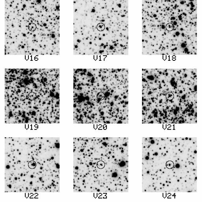
Figure 1: Finding charts for SX Phe variables in M 55. Part I - variables V16 - V24. Each chart is 1 arcmin on a side, with north to the top and east to the left.

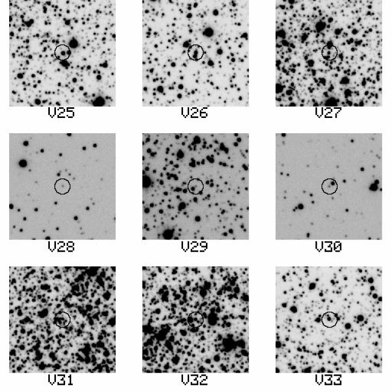
Figure 2: Finding charts for SX Phe variables in M 55. Part II - variables V25 - V33. Each chart is 1 arcmin on a side, with north to the top and east to the left.

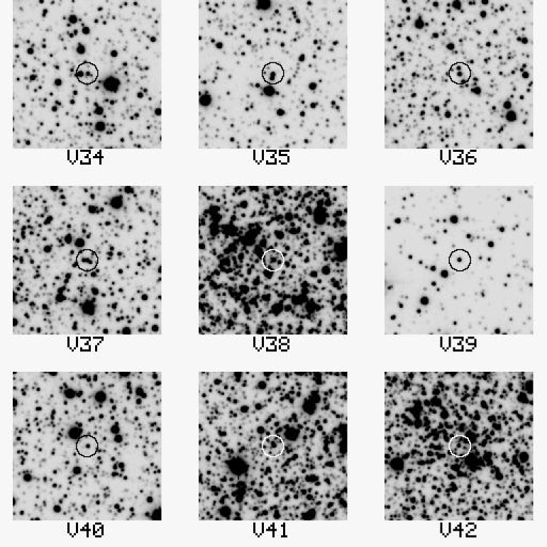
Figure 3: Finding charts for SX Phe variables in M 55. Part III - variables V34 - V42. Each chart is 1 arcmin on a side, with north to the top and east to the left.

We identified 27 SX Phe variables in the field of M 55. Following the nomenclature of Olech et al. (Olech et al. (1999)) the stars are designated as NGC 6809 LCO V16 through NGC 6809 LCO V42. Here-after we use the designations V16 – V42 respectively. Finding charts for these variables are presented in Figs. 1, 2 and 3.

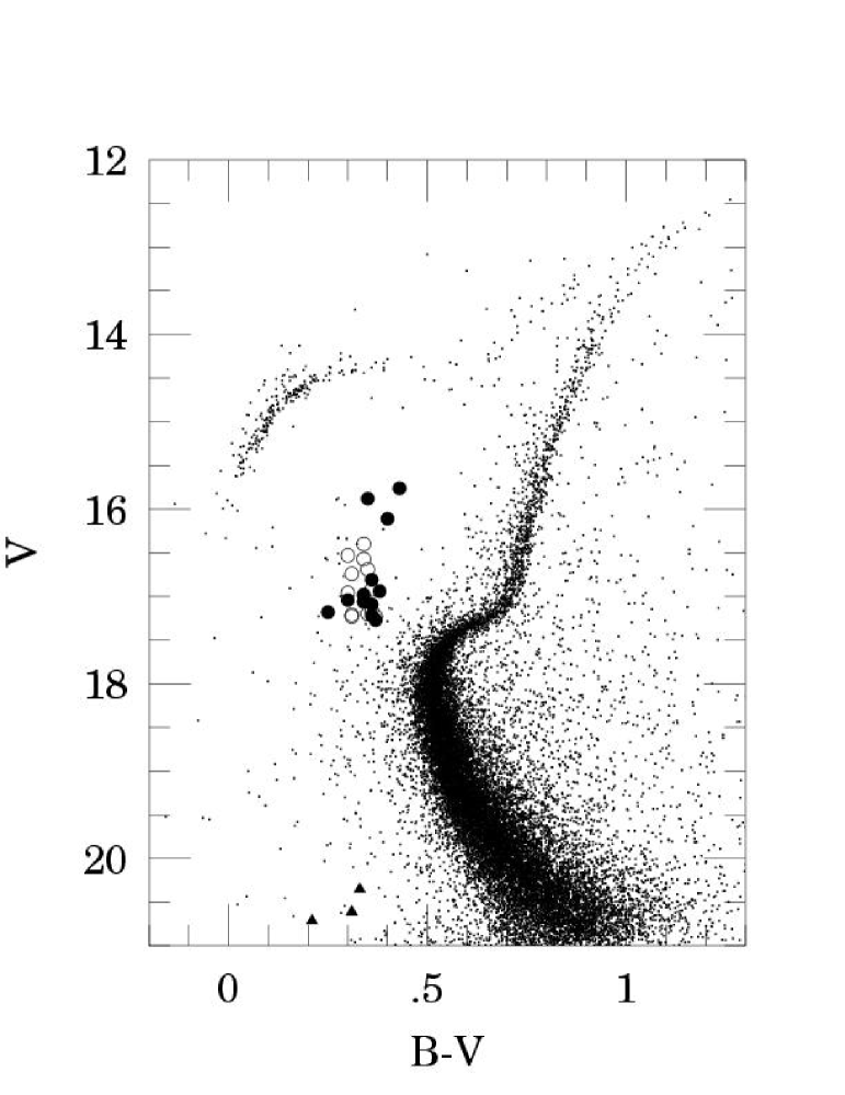
Figure 4: The color-magnitude diagram of the globular cluster M 55. Filled circles denote single-mode SX Phe variables, open circles denote double-mode SX Phe variables, filled triangles denote SX Phe variables from the Sagittarius dwarf galaxy.

The positions of these objects in the color-magnitude diagram are shown in Fig. 4. All of the SX Phe stars belonging to M 55 lie on the blue straggler sequence. Three of the observed SX Phe type stars: V28, V29, V30, are 3.5 – 4 mag fainter than the rest of our sample stars. This difference in magnitude places these 3 stars in the Sagittarius dwarf galaxy (Ibata, Gilmore & Irwin (1994), Fahlman et al. (1996)). The 24 remaining SX Phe variables constitute approximately 50 percent of all the blue straggler stars present in our data.

3.2 Fourier Analysis

Preliminary period estimates were obtained using the CLEAN algorithm (Roberts et al. (1987)). We used a method developed by Schwarzenberg-Czerny (Schwarzenberg-Czerny (1997)) to improve the period determination and to fit a Fourier series to the $V$-band light curves in the form:

$$V=A_{o}+\sum_{j=1}^{k}A_{j}sin(j{\omega}t+\phi_{j})$$ (1)

where $\omega=2{\pi}/P$ and $P$ is the pulsation period of the star. The number of harmonics ($k$) was chosen so that the formal errors of their amplitudes were smaller than the determined values. Since the amplitudes of most of the SX Phe variables in M 55 are smaller than 0.1 mag, for 18/27 stars we were able to measure only the base harmonic ($k=1$). For those stars for which more harmonics could be measured we calculated the Fourier parameters:

$$R_{ij} = A_{i}/A_{j}$$ (2)

$$\Phi_{ij} = i\Phi_{i}-j\Phi_{i}.$$ (3)

In order to help the readers unfamiliar with the AoV periodogram analysis to appreciate the effects of noise and aliasing on our period analysis we provide here as an example description of the light variations of a double mode pulsating star V41 in the terms of the classical power spectrum and window function. The window function looks well as its highest side-lobes due to day and moon cycles do not exceed 83 and 60 percent of the central peak respectively. The window patterns corresponding to the primary and secondary pulsation frequency in the respective original and prewhitened power spectrum are little disturbed and symmetric. Hence our period identifications are unambiguous. The power spectrum remaining after prewhitening with the two detected frequencies and their 5 harmonics is rather flat, consistent with the low frequency calibration errors not exceeding 0.005 mag and no periodic oscillations with amplitudes exceeding 0.004 mag at frequencies exceeding 3 c/d. This is consistent with the theoretical expectations, as any combination amplitudes should be of order of the product of the detected amplitudes i.e. of 0.001 mag. These values for other stars remain within factor of 2 of their respective values for V41.

Standard deviation of the residuals is 0.014 mag, consistent with that expected for the size of the telescope and stellar magnitude. Thus observational errors of an average value of 1/4 all observations should be as small as $\sigma\sim 0.014/\sqrt{180}\sim 0.001$ mag. However, the averages calculated by selecting 1/4 of points around minimum and maximum phases should differ by more than the (half)amplitude of the oscillation, consistent with well over $10\sigma$ significance level of detection even for the secondary oscillation. The AoV statistics used by us tends to yield higher significance levels than the above simple estimate.

3.3 Single mode SX Phe stars

The basic parameters derived for the single-mode oscillators are listed in Table 1, including the variable number, equatorial coordinates (J2000.0), derived periods, mean $V$-band magnitudes, mean $B$-band magnitudes, mean colors ($<$$B$$>-<$$V$$>$), and full amplitudes of the oscillations in $V$. Table 2 presents values of $A_{1}$, $R_{21}$, $\Phi_{21}$, $R_{31}$, $\Phi_{31}$ measured for the single-mode variables. By analogy to Cepheids, we can look for the signature of the resonance between the radial pulsation modes in a $\Phi_{21}$-period plot (Fig. 5). This plot suggests that $\Phi_{21}$ is either constant within the observed period range with a weighted mean of $2.183\pm 0.013$ or slightly increasing with the period, since according to the Fisher-Snedecor test the linear fit $\Phi_{21}=1.954+2.4(\pm 1.0)P$ is marginally better than a constant at confidence level 0.95. Our phases correspond to the sine Fourier series (Eq. 1), for the cosine series the mean phase should be incremented by $\pi/2$. This taken into account, both our constant and linear solutions agree with Poretti (1999). Note that our result is based on a much broader period interval and hence has proportionally stronger weight. The smoothness of the phase does not reveal the presence of any resonance within the range of periods observed here. Curiously, within the errors the same phase difference holds for the principal oscillation of the double mode stars V31 and V32. These were included in the mean value quoted above.

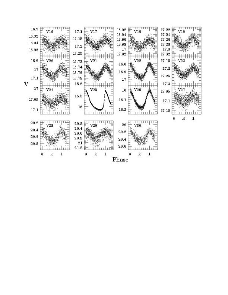
Figure 6: $V$-band light curves for single-mode SX Phe variables observed in the field of M 55

Fig. 6 presents the light curves of the single-mode SX Phe variables observed in the field of M 55.

3.4 Double mode SX Phe stars

We constructed a synthetic light curve for each of the variables using the measured Fourier parameters for that variable. After subtracting this light curve from the observed data points, we searched for a new period with a new fit of a Fourier series. If the full amplitude of the resulting light curve was larger than an arbitrarily chosen value of 0.01 mag, then the object was classified as a double mode variable. Two modes of pulsation were detected in the light curves of 12 of our variables. The parameters for these double-mode SX Phe variables are listed in Table 3, including the variable number, equatorial coordinates (J2000.0), periods of pulsations for both modes, mean $V$-band magnitudes, mean $B$-band magnitudes, mean colors, and full amplitudes in $V$ for the longer period. Table 4 presents the values of $A_{1}^{A}$, $R_{21}^{A}$, $\Phi_{21}^{A}$, $A_{1}^{B}$ measured for the double-mode variables. We use the designations ^A and ^B for the longer and shorter periods, respectively.

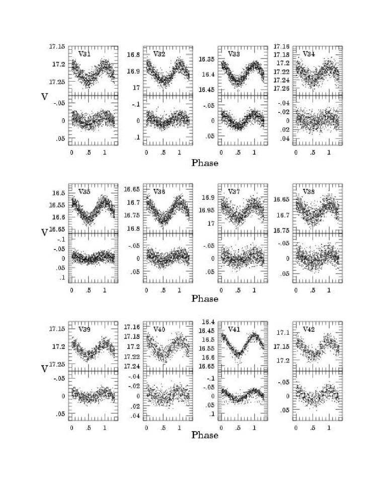
Figure 7: $V$-band light curves for double-mode SX Phe variables observed in the field of M 55. The upper panels show light curves phased with longer period after subtraction of variability with the shorter period approximated by the Fourier series. The lower panels show light curves phased with shorter period after subtraction of variability with the longer period approximated by the Fourier series.

Fig. 7 presents the light curves of the double-mode variables phased with the periods of each mode after prewhitening with the other mode.

4 Mode Identification

Amplitudes generally yield no definitive clues for the identification of modes, except that large amplitudes are more likely to occur in radial pulsations. Our identification of pulsation modes relies on the period ratios and on the distribution of stars in the period-luminosity (P–L) plot.

4.1 Amplitudes

We observe amplitudes ranging from 0.016 mag. to 0.899 mag. The amplitude of V25 ($A_{V}$=0.899 mag) is one of the largest known among all SX Phe type variables. It is not likely that such an amplitude arises in non-radial oscillations. For most of the double-mode variables the amplitude of the longer period oscillations is larger than that for the shorter one. An exception is V38 which has a larger amplitude for the shorter period. For this reason it is very likely that in the double mode stars the oscillations with larger periods and amplitudes are radial (Gilliland et al. (1998)).

In Fig. 8 we present a color-amplitude relation for the stars in our sample. Note that the larger amplitudes are exhibited by stars close to the center of the instability strip. The amplitudes of the double mode stars tend to be smaller than the amplitudes of the single mode stars, but a few single mode stars display very small amplitudes as well. Both effects, if real, are consistent with theoretical expectations. However, the large scatter in Fig. 8 makes any detailed discussion of amplitude effects premature.

4.2 Period Ratios

The periods of the SX Phe variables in M 55 span the range 0.033 to 0.136 days. We use $P_{A}$ for the longer periods and $P_{B}$ for the shorter periods of the double mode variables. Fig. 9 presents $P_{B}/P_{A}$ plotted against $P_{A}$ for the double-mode variables. The $P_{B}/P_{A}$ ratio does not depend on the period of the pulsations. The weighted mean of $P_{B}/P_{A}$ for V31, V32, V33, V34, V37, V38, and V42 is 0.975 $\pm$0.005. The period ratios of V35, V36, V39 and V40 exhibit a larger scatter lying in the range $0.92-0.96$. Since there are no radial modes spaced so closely in frequency, at least one of the modes in our double-mode SX Phe variables is non-radial in origin. However we are unable to say with assurance which of the two modes is radial, if any, using only period information.

4.3 Our Rosetta Stone: V41

V41 is an exceptional case in that its period ratio is extreme compared to other double mode SX Phe stars in M 55 (Fig. 9). This period ratio helps us to identify its pulsation modes with some confidence. The observed value of $0.807\pm 0.009$ is close to the first and second overtone ratio for SX Phe stars (0.801, see Petersen & Høg (1998) for a discussion). For this reason we identify $P_{A}$ and $P_{B}$ with the first and second radial overtones, respectively. In Fig. 10 we plot the period-luminosity relation for the principal periods of all of the stars in our sample. Except for V41 all of the secondary periods of the double-mode stars lay close to their primary periods and are not plotted to avoid confusion. For V41 the secondary period $P_{B}$ lies off of the general P–L relation, toward lower periods. It is consistent with our identification of $P_{B}$ with the second overtone. This is true for all slopes of P–L relations discussed in the literature, ranging from -3.3 to -3.7 (McNamara (1995), McNamara (1997)). However, we caution that these results are extremely sensitive against selection of the observational data. The latter paper claims 5-fold decrease of scatter of $M_{V}$ without explainable improvement in the quality of the observations.

5 The First Overtone P–L Relation

In Fig. 10 the stars V20, V35, V36, V38 and V41 are marked with filled symbols. These stars form a distinct branch away from the main group of SX Phe stars, shifted towards lower periods. Following our identification of V41 as a first overtone pulsator we extend this identification onto the whole group.

Previous investigations have not revealed such a clear separation of the radial modes of SX Phe stars in globular clusters. These investigations have had to rely on small samples from different clusters, and so relative distance errors and spatially variable reddening both introduce significant scatter in the period-luminosity diagram (McNamara (1995), Kaluzny & Krzeminski (1993)).

The dotted line in Fig. 10 represents a linear least squares fit to the first overtone P–L relation:

$$<V>=-3.1 logP_{1}+ 12.32,$$ (4)

$$\pm 0.6 \pm 0.03$$

with a standard residual of the fit of 0.05 mag.

6 The Fundamental Mode P–L Relation for SX Phe Stars

6.1 Slope

We classify all remaining stars in Fig. 10 (plotted with open symbols) as SX Phe stars pulsating in the fundamental mode. The continuous line in Fig. 10 represents a linear least squares fit to this P–L relation:

$$<V>=-2.88 logP_{0} +13.09$$ (5)

$$\pm 0.17 \pm 0.03$$

with a standard residual of the fit of 0.12 mag.

Our fundamental mode P–L relation is less steep than the overtone relation. However the relatively large error of the slope derived for the first overtone P–L relation, does not reject the hypothesis of equal slopes. This is in agreement with the discussion by Nemec et al. (1994). This P–L relation for the fundamental mode stars exhibits a fair amount of scatter. The cause of this might be misidentification among close radial and non-radial modes. The average period ratio of $0.97$ in bimodal stars is consistent with a scatter of 0.03 in $\log P$ due to mode misidentification. In addition, some scatter is to be expected from the finite width of the instability strip.

McNamara (1995) derived a P–L relation with a slope $a=-3.3$ from a compilation of cluster SX Phe stars. This compilation relies on a smaller and less homogeneous data set than that presented here, and hence a realistic estimate of the error of this latter value is expected to be large compared to our error of $0.17$. Thus the McNamara (1995) value for the slope is marginally consistent with our value. A comparison of these results indicates the degree of the external errors involved in P–L relations for SX Phe stars.

Our P–L slope of $a=-2.9$ is inconsistent with the value $a=-3.7$ obtained by Petersen & Høg (1998) from the parallaxes of $\delta$ Scuti stars observed by HIPPARCOS. This is not surprising given the observed scatter in the P–L relation for the HIPPARCOS stars. In addition, these calibrations do not take into account the fact that SX Phe itself is the star in the sample with the shortest period and the lowest metallicity at [Fe/H] = –1.37 (Hintz et al. (1998)). The other 5 $\delta$ Scuti stars from the HIPPARCOS sample have high metallicities ([Fe/H]$\simeq$0.0). Nemec et al. (1994) demonstrated that SX Phe stars follow a period-luminosity-metallicity relation with a coefficient of 0.32 for the [Fe/H] term, and so the slope of the P–L relation from the HIPPARCOS stars will be over-estimated. Our P–L slope is also inconsistent with the value of –3.7 obtained by McNamara (1997) for the highly inhomogeneous sample 26 HADS, for which P–L dependence was found indirectly, via many intermediate steps.

6.2 Zero point

On the other hand the HIPPARCOS parallax of SX Phe is crucial for a determination of the zero point of the P–L relation for our M 55 stars. The metallicity of SX Phe is similar to M 55 ([Fe/H]$=-1.54$, Rutledge et al. (1997)). The parallax of SX Phe ($\pi=12.91$ miliarcsec) is well determined with a relative error $\sigma_{\pi}/\pi=0.06$. The absolute magnitude of the SX Phe, derived using the HIPPARCOS parallax, is $M_{V}=2.88\pm 0.13$ mag (Petersen & Høg (1998)). Oudmajier et al. (1998) determined that when the relative error of the parallax is smaller than about 0.15, the Lutz-Kelker correction (Lutz & Kelker (1973)) accurately describes the probable shift in the derived absolute magnitude. In the case of SX Phe, the Lutz-Kelker correction is equal to $-0.02$ mag, so the corrected absolute magnitude is $2.86$ mag. This value, when combined with Eq. (5) for the fundamental mode period of SX Phe of $P_{0}=0.0550$ days (Petersen & Høg (1998)), yields our final P–L relation:

$$M_{V}=-2.88 logP_{0} -0.77$$ (6)

$$\pm 0.17 \pm 0.25$$

Using our calibration we determine the apparent distance modulus to M 55 to be $(m-M)_{V}=13.86\pm 0.25$ mag. This result is consistent with the apparent distance to M 55 determined from the analysis of RR Lyrae stars in M 55 by Olech et al. (1999).

7 The Period–Color Relation

$\delta$ Scuti and SX Phe stars close to the red border of the instability strip have periods significantly longer than the periods of stars at the center of the strip (Pamiatnykh (2000)). The period-color ($logP/(V-I)$) dependence for $\delta$ Scuti stars from the Galactic Bulge was described by Mcnamara et al. (2000). A linear least squares fit to our data, presented in Fig. 11 yields the following relation:

$$<B-V>=0.15 logP +0.543$$ (7)

$$\pm 0.05 \pm 0.008$$

The standard residuals from the fit amount to $0.05$ mag. Note that the star towards lower right in Fig. 10 is V21, which is found at the extreme red border of the instability strip (Fig. 4). Any attempt to account for this by including a color term in the P–L relation failed to improve the quality of the fit.

8 Conclusions

SX Phe type variables seem to be good distance indicators. Although their luminosities are too low for investigations in distant galaxies, they are bright enough to be observed in nearby galaxies. The largest number of SX Phe variables in one globular cluster was found in $\omega$ Cen (Kaluzny et al. (1996), Kaluzny et al. 1997a ), but due to its varying metallicity this cluster is not suitable for distance calibration. In M 55 we discovered the richest population of SX Phe among the rest of globular clusters. M 55 is thought to be chemically homogeneous (Richter, Hilker & Richtler (1999)). This enabled a separation of the fundamental and first overtone stars and an estimate of the errors caused by misidentification of nearby radial non-radial frequencies. In this way we obtained a reliable slope of the P–L relation for the fundamental mode stars. Combined with the HIPPARCOS parallax for SX Phe itself, we obtain an improved P–L relation (Eq. 6). Despite being based on just one star, our zero point should be reliable as HIPPARCOS parallax of SX Phe has an error of $6$ percent and metallicities of SX Phe and of M 55 are as close as $-1.37$ and $-1.54$. Using our revised P–L relation for SX Phe stars we measure the apparent distance to M 55 to be $(m-M)_{V}=13.86\pm 0.25$ mag.

Table 1: List of single-mode SX Phe variables in the field of M 55

star	R.A.(J2000.0)	Dec.(J2000)	P	$<V>$	$<B>$	$<$$B$$>-<$$V$$>$	$A_{V}$
	hh:mm:sec	deg:’:”	[days]
V16	19:40:09.20	-30:56:42.04	0.0534204(8)	16.94	17.32	0.38	0.016
V17	19:40:11.33	-30:59:25.06	0.0412615(3)	17.18	17.43	0.25	0.049
V18	19:40:06.87	-30:56:32.12	0.0465555(4)	16.98	17.32	0.34	0.029
V19	19:39:57.67	-30:57:01.31	0.0382367(2)	17.27	17.64	0.37	0.033
V20	19:39:54.95	-30:58:21.25	0.0332118(2)	17.04	17.34	0.30	0.102
V21	19:39:58.27	-30:59:06.05	0.1355924(2)	15.76	16.19	0.43	0.036
V22	19:40:07.80	-31:00:12.60	0.0456394(1)	16.81	17.17	0.36	0.337
V23	19:39:51.82	-30:55:52.83	0.0413989(3)	17.22	17.58	0.36	0.050
V24	19:39:45.49	-30:56:02.68	0.0418206(5)	17.06	17.40	0.34	0.026
V25	19:39:51.55	-30:56:21.27	0.0985309(1)	15.88	16.23	0.35	0.899
V26	19:39:47.06	-30:57:33.98	0.0820096(2)	16.11	16.51	0.40	0.173
V27	19:39:54.05	-30:58:07.46	0.0410265(5)	17.09	17.45	0.36	0.029
V28*	19:40:15.04	-31:05:15.03	0.0537630(6)	20.61	20.92	0.31	0.260
V29*	19:39:42.58	-30:55:58.34	0.0343115(2)	20.71	20.92	0.21	0.295
V30*	19:39:41.02	-30:50:25.23	0.0563464(5)	20.35	20.68	0.33	0.258

* Probable member of the Sagittarius dwarf galaxy.

Table 2: Fourier parameters of single-mode SX Phe variables in M 55. See Eqs. (2) and (3) for the definition.

star	$A_{1}$	$R_{21}$	${\phi}_{21}$	$R_{31}$	${\phi}_{31}$
V16	0.0079 ${\pm}$0.0005	-	-	-	-
V17	0.0246 ${\pm}$0.0009	-	-	-	-
V18	0.0144 ${\pm}$0.0006	-	-	-	-
V19	0.0166 ${\pm}$0.0006	-	-	-	-
V20	0.0500 ${\pm}$0.0016	0.126 ${\pm}$0.033	2.33 ${\pm}$0.27	-	-
V21	0.0178 ${\pm}$0.0004	0.125 ${\pm}$0.021	2.55 ${\pm}$0.17	-	-
V22	0.1609 ${\pm}$0.0023	0.250 ${\pm}$0.015	2.06 ${\pm}$0.06	-	-
V23	0.0252 ${\pm}$0.0008	-	-	-	-
V24	0.0130 ${\pm}$0.0007	-	-	-	-
V25	0.3454 ${\pm}$0.0008	0.480 ${\pm}$0.003	2.19 ${\pm}$0.01	0.240 ${\pm}$0.003	4.50 ${\pm}$0.01
V26	0.0839 ${\pm}$0.0006	0.221 ${\pm}$0.007	2.16 ${\pm}$0.03	0.034 ${\pm}$0.007	4.66 ${\pm}$0.21
V27	0.0143 ${\pm}$0.0009	-	-	-	-
V28	0.1276 ${\pm}$0.0047	0.190 ${\pm}$0.038	2.01 ${\pm}$0.21	-	-
V29	0.1477 ${\pm}$0.0063	-	-	-	-
V30	0.1191 ${\pm}$0.0042	0.321 ${\pm}$0.036	2.13 ${\pm}$0.13	0.132 ${\pm}$0.034	4.59 ${\pm}$0.28

Table 3: List of double-mode SX Phe variables in M 55

star	R.A.(J2000.0)	Dec.(J2000.)	$P_{A}$	$P_{B}$	$<V>$	$<B>$	$<$$B$$>-<$$V$$>$	$A_{V}$($P_{A}$)
	hh:mm:sec	deg:’:”	[days]	[days]
V31	19:40:00.99	-30:57:56.53	0.0388471(2)	0.0382042(5)	17.23	17.60	0.37	0.041
V32	19:39:58.14	-30:58:32.66	0.0414874(2)	0.0405483(5)	16.92	17.28	0.36	0.097
V33	19:39:54.56	-30:59:57.88	0.0593067(3)	0.0573473(4)	16.40	16.74	0.34	0.054
V34	19:40:01.02	-31:00:37.93	0.0370203(3)	0.0360939(6)	17.23	17.54	0.31	0.029
V35	19:39:50.37	-30:55:12.41	0.0486858(2)	0.0452695(7)	16.57	16.91	0.34	0.070
V36	19:39:48.56	-30:56:45.04	0.0393958(2)	0.0373768(4)	16.74	17.05	0.31	0.067
V37	19:39:49.87	-30:57:42.53	0.0437976(3)	0.0428239(7)	16.96	17.26	0.30	0.051
V38	19:39:58.86	-30:58:14.78	0.0391971(5)	0.0381747(3)	16.69	17.04	0.35	0.044*
V39	19:40:11.99	-31:02:04.48	0.0358151(3)	0.0341535(5)	17.21	17.52	0.31	0.034
V40	19:40:01.90	-30:55:38.20	0.0369762(4)	0.0346515(7)	17.20	17.56	0.35	0.028
V41	19:40:02.95	-30:58:28.34	0.0451669(2)	0.0364552(3)	16.53	16.83	0.30	0.106
V42	19:39:58.61	-30:57:23.93	0.0366655(3)	0.0356382(5)	17.16	17.52	0.36	0.053

* Amplitude of $P_{B}$ pulsations (see text)

Table 4: Fourier parameters of double-mode SX Phe variables in M 55. See Eqs. (2) and (3) for the definition.

star	$A_{1}^{A}$	$R_{21}^{A}$	${\phi}_{21}^{A}$	$A_{1}^{B}$
V31	0.0204 ${\pm}$0.0006	0.074 ${\pm}$0.029	1.19 ${\pm}$0.40	0.0093 ${\pm}$0.0006
V32	0.0478 ${\pm}$0.0011	0.143 ${\pm}$0.023	2.20 ${\pm}$0.17	0.0194 ${\pm}$0.0011
V33	0.0271 ${\pm}$0.0005	-	-	0.0181 ${\pm}$0.0005
V34	0.0144 ${\pm}$0.0006	-	-	0.0060 ${\pm}$0.0006
V35	0.0349 ${\pm}$0.0007	-	-	0.0099 ${\pm}$0.0008
V36	0.0333 ${\pm}$0.0007	-	-	0.0119 ${\pm}$0.0007
V37	0.0254 ${\pm}$0.0009	-	-	0.0106 ${\pm}$0.0009
V38	0.0122 ${\pm}$0.0008	-	-	0.0218 ${\pm}$0.0008
V39	0.0170 ${\pm}$0.0006	-	-	0.0080 ${\pm}$0.0006
V40	0.0141 ${\pm}$0.0006	-	-	0.0068 ${\pm}$0.0006
V41	0.0532 ${\pm}$0.0008	-	-	0.0243 ${\pm}$0.0008
V42	0.0263 ${\pm}$0.0010	-	-	0.0171 ${\pm}$0.0010

Figure 5: $\phi_{21}$-period relation for SX Phe stars in M 55.

Figure 8: The color-amplitude relation for SX Phe stars in M 55. Squares denote single mode pulsators, triangles denote double mode pulsators.

Figure 9: Period ratio ($P_{B}/P_{A}$) versus $P_{A}$ relation for double mode SX Phe variables in M 55. The open symbols represent the stars with the period ratios $0.9<P_{B}/P_{A}<1.0$ - at least one of the modes must be non-radial. The filled circle denotes V41 with the period ratio equal to 0.807 - characteristic for pulsations in the first and the second radial overtones.

Figure 10: The period-luminosity dependence for SX Phe stars in M 55. The squares denote single-mode variables, the triangles denote points corresponding to longer periods of double-mode variables, the circle denotes the point corresponding to the second overtone period of V41. The solid line represents linear least squares fit to the points marked with open symbols (fundamental mode pulsators). The dashed line represents linear least squares fit to the points marked with filled symbols (first overtone pulsators). The horizontal line represents the period shifts of V41: between the first and the second overtones, and to the fundamental mode.

Figure 11: The period-color dependence for SX Phe stars in M 55. The squares denote single-mode variables, the triangles denote points corresponding to longer periods of double-mode variables. The solid line represents linear least squares fit drawn through the plotted points.