Optical Spectroscopy of Type Ib/c Supernovae

Abstract

We present 84 spectra of Type Ib/c and Type IIb supernovae (SNe), describing the individual SNe in detail. The relative depths of the helium absorption lines in the spectra of the SNe Ib appear to provide a measurement of the temporal evolution of the SN, with He I $\lambda$5876 and He I $\lambda$7065 growing in strength relative to He I $\lambda$6678 over time. Light curves for three of the SNe Ib provide a sequence for correlating the helium-line strengths. We find that some SNe Ic show evidence for weak helium absorption, but most do not. Aside from the presence or absence of the helium lines, there are other spectroscopic differences between SNe Ib and SNe Ic. On average, the O I $\lambda$7774 line is stronger in SNe Ic than in SNe Ib. In addition, the SNe Ic have distinctly broader emission lines at late times, indicating either a consistently larger explosion energy and/or lower envelope mass for SNe Ic than for SNe Ib. While SNe Ib appear to be basically homogeneous, the SNe Ic are quite heterogeneous in their spectroscopic characteristics. Three SNe Ic that may have been associated with gamma-ray bursts are also discussed; two of these have clearly peculiar spectra, while the third seems fairly typical.

1 Introduction

Since Minkowski (1941) first differentiated supernovae (SNe) into two classes based on the absence (Type I) or presence (Type II) of hydrogen lines in their spectra, SNe have traditionally been classified by their spectroscopic characteristics near maximum brightness. The hydrogen-poor Type I SNe appeared initially to be a very homogeneous class, but some subtle differences were gradually noticed. The Type I class was thus split into subtypes. The most distinctive feature of the prototypical Type I SNe—now referred to as Type Ia SNe (or SNe Ia)—is a strong absorption line near 6150 Å that is the result of blueshifted Si II $\lambda\lambda$6347, 6371 (often referred to jointly as $\lambda$6355). The other Type I subtypes lack this 6150 Å feature and are discriminated by the presence (SNe Ib) or absence (SNe Ic) of He I lines; other than this difference, Types Ib and Ic are very similar. The nebular-phase spectra of the various types are also distinctive. Type II SNe continue to be dominated by Balmer emission, but also show lines of neutral and singly-ionized oxygen and calcium. The late-time spectra of Type Ia SNe consist mainly of many overlapping lines of iron and cobalt. Types Ib and Ic have spectra that are quite similar to those of late-time Type II SNe, but without the hydrogen lines. For a more thorough review of the history and details of SN classification and spectroscopy, see, e.g., Harkness & Wheeler (1990), Branch (1990), and Filippenko (1997).

These spectroscopic differences reflect the nature of the progenitors for each of the SN types. The evolution of the spectra of Type Ia SNe, along with their environments and homogeneous light curves, has led to a general consensus that they are the result of the thermonuclear disruption of a white dwarf (see, e.g., Branch et al. 1995). By a similar line of reasoning, Type II SNe arise from the core collapse of massive ($\gtrsim 8-10$ M_☉) stars (e.g., Woosley & Weaver 1986; Arnett et al. 1989). The progenitors of Type Ib and Ic SNe were not as clear, as the basic data needed to characterize the SNe themselves were limited (see Harkness & Wheeler 1990 and Clocchiatti et al. 1997 for more details).

Evidence gradually began to accumulate that the Type Ib and Ic SNe were related to Type II SNe. Type Ib/c SNe and Type II SNe appear in similar environments (Van Dyk, Hamuy, & Filippenko 1996, and references therein); in addition, Type Ib/c SNe occur almost exclusively in late-type galaxies (Porter & Filippenko 1987) and they often exhibit radio emission that is thought to arise from circumstellar interaction (e.g., Weiler et al. 1998, and references therein). As mentioned above, the late-time spectra of Type Ib/c SNe are very similar to those of Type II SNe, but without the hydrogen. Thus, it is likely that the progenitors of Type Ib/c SNe are also massive stars, although white dwarf progenitor models have been considered (e.g., Branch & Nomoto 1986; Iben et al. 1987).

More direct evidence for the connection between Type Ib/c SNe and Type II SNe is provided by several SNe that have transformed from one spectral type into another. The first of these was SN 1987K. It was initially classified as a Type II SN, but later observations showed no hydrogen lines; the actual metamorphosis was not observed (Filippenko 1988). Woosley et al. (1987) had already considered such a scenario and had suggested the new name of “Type IIb.” SN 1993J was also a Type II SN when first observed, but then developed the He I lines of a Type Ib (e.g., Filippenko, Matheson, & Ho 1993; Wheeler & Filippenko 1996; Matheson et al. 2000a, and references therein). Qiu et al. (1999) show a similar transformation for SN 1996cb. These observed metamorphoses provide a clear link between the Type II SNe and Type Ib/c SNe. The hydrogen missing from the spectra of Type Ib/c SNe is thought to have been lost from the progenitor through winds or mass transfer to a companion (e.g., Woosley, Langer, & Weaver 1993; Yamaoka, Shigeyama, & Nomoto 1993; Nomoto et al. 1994; Iwamoto et al. 1994; for SN 1993J specifically, see Woosley et al. 1994; Wheeler & Filippenko 1996; Matheson et al. 2000a, and references therein).

The differences between progenitors that yield Type Ib SNe and Type Ic SNe remain uncertain. It may be that the same mechanism of mass transfer invoked above to explain the disappearance of hydrogen can also remove the helium from a star that then explodes as a Type Ic SN. SN 1999cq, a Type Ic based on its spectrum, exhibited intermediate-width He I emission lines that might represent the interaction of the ejecta with dense clumps of almost pure helium (no Balmer lines were present; Matheson et al. 2000b). This could be a direct detection of the helium layer that was in the process of being lost by the progenitor. Some Type Ic SNe, however, still show broad helium lines. There have been claims of the He I $\lambda$10830 line in SN 1990W (Wheeler et al. 1994), SN 1994I (Filippenko et al. 1995), and SN 1994ai (Benetti, quoted in Clocchiatti et al. 1997). Wheeler et al. (1994) suggest that the presence of this line makes SN 1990W a Type Ib SN instead, highlighting the difficulty in distinguishing between SNe Ib and SNe Ic. Reanalysis of other Type Ic SNe spectra has also shown some indications of several helium lines (Clocchiatti et al. 1996; Munari et al. 1998), although other studies have countered these claims (Baron et al. 1999; Millard et al. 1999).

The difficulty of exciting helium to produce lines may provide an alternative cause for the differences between Type Ib and Ic SNe. Gamma rays emitted by newly synthesized ⁵⁶Ni accelerate electrons that then act as a source of nonthermal excitation for helium (Harkness et al. 1987; Lucy 1991). Thus, helium could still be present in both Type Ib and Ic SNe, but lines are only observed if the nickel is mixed into the the helium layer in quantities sufficient to excite the helium (e.g., Wheeler et al. 1987; Shigeyama et al. 1990; Hachisu et al. 1991).

To help resolve the controversy over the nature of SNe Ib and SNe Ic, we studied the aggregate collection of spectra of stripped-envelope SNe (Types Ib, Ic, and IIb) that the SN group at U.C. Berkeley has obtained in the past 12 years. Some of these spectra, notably those of SN 1994I and SN 1993J, have been presented in detail elsewhere (Filippenko et al. 1995; Filippenko, Matheson, & Ho 1993; Filippenko, Matheson, & Barth 1994; Matheson et al. 2000a). Discounting them, the sample consists of 84 spectra of SNe Ib, Ic, and IIb. There are also spectra of three SNe initially classified as SNe Ib/c, but whose characteristics indicate that they are in fact SNe Ia. In §2 the observations are described in general; the individual SNe are presented in detail in §3. The evolution of the spectra of SNe Ib is discussed in §4.1. Helium lines in SNe Ic are considered in §4.2. Some spectroscopic distinctions of SNe Ib and SNe Ic are shown in §4.3. The evolution and heterogeneity of SNe Ic are highlighted in §4.4, with a special emphasis on two peculiar SNe Ic in §4.5 that may be associated with gamma-ray bursts.

2 Observations

Low-dispersion spectra of the SNe Ib/c considered here were obtained with a variety of instruments. The majority were observed at the Cassegrain focus of the Shane 3-m reflector at Lick Observatory, using either the original CCD spectrograph (the “UV Schmidt”; Miller & Stone 1987) up to the 1992 January 09 data or the Kast double spectrograph (Miller & Stone 1993) from 1992 March to the present. Several spectra were also obtained with the double spectrograph on the Hale 5-m reflector at Palomar Observatory (Oke & Gunn 1982) and with the Low Resolution Imaging Spectrometer (LRIS; Oke et al. 1995) at the Keck II 10-m telescope. A single spectrum was observed with the Kitt Peak Mayall 4-m telescope using the RC spectrograph. A long, narrow (typically 2$\arcsec$, but smaller for the LRIS observations) slit was used. Various gratings and grisms were utilized, yielding resolutions (full width at half maximum, FWHM) ranging from 6 Å to 15 Å. Details of the exposures are given in Table 1. Most of the spectra were taken with the slit oriented at, or near (within 10^∘), the parallactic angle (Filippenko 1982).

Standard CCD processing and spectrum extraction were accomplished with VISTA (Terndrup, Lauer, & Stover 1984) or IRAF. Optimal extraction was used for the IRAF reductions (Horne 1986). The wavelength scale was established using low-order polynomial fits to spectra of calibration lamps. The typical root-mean-square (rms) deviation for the wavelength solution was $0.1-0.5$ Å, depending on the resolution for the particular exposure. Final adjustments to the wavelength scale were obtained by using the background sky regions to provide an absolute scale. We employed our own routines to flux calibrate the data; comparison stars are listed in Table 1. Particular care was taken to remove telluric absorption features through division by an intrinsically featureless spectrum, where possible (Wade & Horne 1988). The flux standard was routinely employed for this purpose. While the relative spectrophotometry is excellent (individual exceptions are noted in the discussion below), no attempt has been made to calibrate the fluxes to an absolute scale.

For four of the SNe (1998dt, 1998fa, 1999di, and 1999dn), we have photometric observations obtained with the 0.75-m Katzman Automatic Imaging Telescope at Lick Observatory (KAIT; Treffers et al. 1997; Richmond, Treffers, & Filippenko 1993; Li et al. 2000; Filippenko et al. 2001). The detector used by KAIT is a SITe $512\times 512$ pixel CCD with a field of view of 6.′8 $\times$ 6.′8. For SN 1998dt, we used a point-spread function (PSF) fitting technique to measure magnitudes. SN 1998fa, SN 1999di, and SN 1999dn were in complex regions of their host galaxies. We therefore employed a galaxy subtraction method to isolate the SNe; magnitudes were then determined using PSF fitting. Not all of the SNe were followed with standard $UBVRI$ filters. Their host galaxies, though, are part of the Lick Observatory Supernova Search (LOSS; Li et al. 2000; Filippenko et al. 2001) and thus are imaged regularly (every three to four days). These observations are taken without a filter, yielding unfiltered magnitudes. Photometric calibration of KAIT images indicates that the unfiltered response is similar to (but broader than) that of a standard $R$ filter (Riess et al. 1999; the KAIT $R$ filter is a Bessell $R$ [Bessell 1990]). For SNe 1998dt and 1999dn, there was photometric coverage with the $R$-band filter, and the unfiltered observations match the $R$ light curve quite well. Therefore, we will use both $R$-band and unfiltered magnitudes to construct light curves for the SNe. The differences between $R$-band and unfiltered observations may increase as the spectrum becomes more line-dominated, since the edges of the two passbands may include different sets of lines. The chief use of the light curves, however, is to provide a temporal order for the spectra, so it is the epoch of maximum light that is most important, and the measured magnitudes from the two passbands roughly agree at this phase for the SNe with $R$-band and unfiltered coverage.

3 Description of Individual Supernovae

Throughout this section, the magnitude of the SN at the time of discovery is quoted directly from the I.A.U. Circulars. The systems used to detect the SNe are very heterogeneous, with most using unfiltered observations. None of the numbers reported is well-calibrated on a standard system and some may have large uncertainties. They should only be used as rough indicators of relative brightness. All calendar dates reported are UT. In all the figures of the SNe spectra, the systemic heliocentric velocity has been removed. If a velocity could be determined from narrow emission lines in the SN spectrum (from superposed H II regions) then that value was used; if not, then the velocity of the host galaxy (i.e., of the nucleus) was removed. If the velocity of the host galaxy was found from our spectra, this is explicitly mentioned. Otherwise, a reference to the source for the galactic velocity is given or, for most NGC, UGC, or IC objects, we describe it as a “listed” velocity taken from the de Vaucouleurs et al. (1991) RC3 catalog.

SN 1988L.—This supernova was discovered in the course of the Berkeley Automated Supernova Search (BASS) on 1988 April 30 at a magnitude of 16.5 (Perlmutter & Pennypacker 1988) in NGC 5480. The narrow H$\alpha$ emission line from a superposed H II region is observed at 6608 Å, yielding a recession velocity of 2050 km s^-1; the velocity of NGC 5480 is listed as 1856 km s^-1. It was initially classified as Type I (possibly Ia or Ib; Graham, Boroson, & Oke 1988), and finally confirmed as Type Ib (Filippenko, Spinrad, & McCarthy 1988; Kidger 1988). Some of these spectra have already been published (Filippenko 1988). Our first spectrum (1988 May 11; Figure 1) is eleven days after discovery, and still in the photospheric phase. The later spectra exhibit the typical nebular lines of Type Ib/c SNe, namely [O I] $\lambda\lambda$6300, 6364, [Ca II] $\lambda\lambda$7291, 7324, O I $\lambda$7774, and the calcium near-infrared (near-IR) triplet.

SN 1990B.—The BASS also discovered this SN on 1990 January 20 in NGC 4568 at a magnitude of 16 (Perlmutter & Pennypacker 1990). We find a recession velocity for the SN of 2200 km s^-1 from narrow H$\alpha$ emission from an H II region, while the listed galactic velocity for NGC 4568 is 2255 km s^-1. The lack of hydrogen lines indicated that the SN was of Type I (Dopita & Ryder 1990), and subsequent spectra confirmed that it was a SN Ib (Filippenko, Spinrad, & Dickinson 1990; Kirshner & Leibundgut 1990; Benetti, Cappellaro, & Turatto 1990a). Later analysis indicated that SN 1990B was actually a Type Ic SN (Clocchiatti et al. 2001); at the earlier stages, the existence of a separate subclass of helium-poor Type I SNe (i.e., the SNe Ic) had yet to be demonstrated. Radio emission was also detected from SN 1990B (Sramek, Weiler, & Panagia 1990; Van Dyk et al. 1993). Some of the spectra shown here (Figure 2) are also presented by Clocchiatti et al. (2001). Our first three spectra (1990 January 23, February 10, and February 27) show some absorption features, but they do not exhibit the full set of helium lines that would indicate a SN Ib; thus SN 1990B is a SN Ic according to our spectra; see, however, §4.2. By 1990 March 25, the SN had begun to enter the nebular phase.

SN 1990U.—Another BASS discovery, SN 1990U was found on 1990 July 27 in NGC 7479 at magnitude 16 (Pennypacker, Perlmutter, & Marvin 1990). Narrow H$\alpha$ emission from an H II region indicates a recession velocity of 2500 km s^-1 with a listed galactic velocity of 2378 km s^-1. It was initially classified as a SN Ib (Filippenko & Shields 1990a). The relative weakness (or absence) of the He I lines led to a re-evaluation of the object as a Type Ic (Filippenko & Shields 1990b). As can be seen in Figure 3, there are features in the photospheric spectra, but the He I lines are not prominent.

SN 1990aa.—The BASS found SN 1990aa on 1990 September 4 at magnitude 17 in UGC 540. The recession velocity of the SN based on the narrow H$\alpha$ emission line from an H II region is 5020 km s^-1 while the listed velocity for UGC 540 is 4982 km s^-1. The preliminary classification was as Type Ia (Della Valle 1990; Benetti, Cappellaro, & Turatto 1990b), but it was recognized as a SN Ib, or possibly SN Ic, with fully calibrated spectra (Filippenko & Shields 1990b). Our spectra (Figure 4) show that this is a SN Ic; there are many features in the 1990 September 27 spectrum, but the He I lines are not present at great strength, if at all.

SN 1990aj.—McNaught (1991a) discovered SN 1990aj on a plate taken 1990 December 19 at magnitude 18 in NGC 1640. Pre-discovery images showed it on 1990 December 6. There are no visible (H II region) narrow emission lines, but the centroid of the [O I] $\lambda\lambda$6300, 6364 line gives a velocity of 1900 km s^-1; the listed recession velocity of NGC 1640 is 1602 km s^-1. The supernova’s spectral features indicated that it was a late-time SN Ib (Della Valle & Pasquini 1991), but without photospheric spectra, it is unclear whether this was a SN Ib or SN Ic. Our spectrum only shows the late nebular lines of a SN Ib/c (Figure 5).

SN 1991A.—The BASS discovered SN 1991A on 1991 January 1 at magnitude 18 in IC 2973 (Pennypacker et al. 1991). Narrow H$\alpha$ emission from an H II region gives a recession velocity of 3250 km s^-1 while the listed galactic value is 3206 km s^-1. It was classified as a Type Ic SN (Filippenko 1991a), with the possibility of a weak H$\alpha$ component (Filippenko 1991b). This broad feature near H$\alpha$ is visible in our spectra (Figure 6). The rest of the spectrum is relatively featureless between 6000 and 7500 Å. The 1991 January 17 spectrum shows an apparent double minimum between 5500 Å and 5800 Å. The redward minimum is most likely Na I D, while the blueward one may be He I $\lambda$5876; see the discussion of helium in SNe Ic in §4.2

SN 1991D.—SN 1991D was discovered by Remillard et al. (1991) on 1991 February 6 at magnitude $\sim$ 16.5 in an anonymous galaxy. This galaxy was actually number 23 of List 1 of the Calán-Tololo Seyfert Galaxies (Maza & Ruiz 1989), also known as PGC/LEDA 84044. There are no narrow (H II region) emission lines in the spectrum of the SN, but the redshift of the host galaxy is $\sim$ 12500 km s^-1 (Maza & Ruiz 1989). The discoverers’ own spectrum indicated it was of Type I. Later spectra showed that it was a SN Ib or SN Ic (Kirshner, Huchra, & McAfee 1991), but most likely a Type Ib (Filippenko & Shields 1991b). Figure 7 shows the spectrum obtained by Remillard et al. (1991; the 1991 February 7 spectrum), as well as our own. The wavelength coverage of the 1991 February 7 spectrum is not extensive, but He I $\lambda$7065 and $\lambda$7281 are visible, and there are hints of those lines in the February 23 spectrum as well, lending credence to the classification as a SN Ib. The poor signal-to-noise (S/N) ratio of the spectra does hamper a definitive classification.

SN 1991K.—McNaught (1991b) discovered SN 1991K on 1991 February 21 in NGC 2851 at a magnitude of 18. This SN shows no narrow (H II region) emission lines in its spectrum. The recession velocity of NGC 2851 is 5096 km s^-1 (Phillips 1991a). There was some confusion about the classification of this object. The first spectra were consistent with Type II or Type Ic (Filippenko & Shields 1991a), but subsequent reports indicated Type Ib (Phillips 1991a). Late-time spectra ($\gtrsim$ 100 days), however, resemble those of Type Ia SNe (Gómez, López, & Sánchez 1996). Our spectra, one of which is seen in Figure 8, show a striking similarity with a normal Type Ia SN at later times.

SN 1991L.—Pollas (1991) discovered SN 1991L on plates taken 1991 February 24 at magnitude 18 in MCG +07-34-134. While the spectrum of SN 1991L shows no narrow (H II region) emission lines, the narrow H$\alpha$ emission from our spectrum of the galaxy nucleus gives a recession velocity of 9050 km s^-1. Filippenko, Shields, & Nomoto (1991) classified the SN as a Type Ib or Ic. The fully calibrated spectrum (Figure 9), however, does not stand out as a clear example of any known type of SN. The features at the blue end are reminiscent of SNe Ia (cf. Figure 8), but the iron features that dominate this region are common to all SN types. In addition, the lack of the Si II absorption belies a SN Ia claim. The peculiar, overluminous Type Ia SN 1991T had a very weak silicon line at early times (Filippenko et al. 1992a; Phillips et al. 1992), but the rest of the spectrum does not match that of SN 1991L. With just this one spectrum, the exact nature of SN 1991L will remain a mystery, but it is probably a SN Ib or SN Ic.

SN 1991N.—The BASS found SN 1991N on 1991 March 29 at magnitude 15 in NGC 3310 (Perlmutter et al. 1991). It was classified as a Type Ic (possibly Type Ib; Filippenko 1991c). This SN is superposed on a very bright H II region. The recession velocity derived from the narrow emission lines of the H II region is 1190 km s^-1, while that of NGC 3310 is listed as 980 km s^-1. Figure 10 shows our spectra of SN 1991N. The photospheric spectra are relatively smooth in the range 6000$-$7500 Å where most of the distinctive He I lines are found, indicating that this is definitely a SN Ic. The spectra of SN 1991N are heavily contaminated by starlight, as indicated by the very blue late-time spectra.

SN 1991ar.—SN 1991ar was found by McNaught (1991c) on 1991 September 3 at magnitude 17 in IC 49. The SN has a recession velocity of 4520 km s^-1 based on the narrow (H II region) H$\alpha$ emission line. The listed velocity of IC 49 is 4562 km s^-1. Phillips (1991b) classified it as a Type Ib; this was confirmed by Filippenko & Matheson (1991b), despite an earlier misidentification as a Type II (Filippenko & Matheson 1991a). Our spectra (Figure 11), although noisy, show distinctly the He I series.

SN 1995F.—Lane & Gray (1995) discovered SN 1995F on 1995 February 11 at a magnitude of $\sim$ 15 in NGC 2726. The narrow (H II region) H$\alpha$ emission line in the spectra of this SN indicates a recession velocity of 1440 km s^-1, while the listed galactic value for NGC 2726 is 1518 km s^-1. It was classified as a Type Ic (possibly Type Ib; Filippenko & Barth 1995). The photospheric spectra of SN 1995F (Figure 12) show many features, but they are not at the correct wavelengths to be helium, so the object is a SN Ic.

SN 1995bb.—During the course of a redshift survey, Tokarz & Garnavich (1995) found SN 1995bb in a spectrum of an anonymous galaxy taken on 1995 November 29. The spectrum indicated the nebular features of a Type Ib/c SN. We find a recession velocity for SN 1995bb of 1610 km s^-1 based on the narrow (H II region) H$\alpha$ emission line in the spectrum, in contrast to the value of 1740 km s^-1 reported by Tokarz & Garnavich (1995). Figure 13 displays our spectrum, which shows only the nebular-phase lines of [O I] $\lambda\lambda$6300, 6364 and Mg I] $\lambda$4571.

SN 1996cb.—SN 1996cb was discovered by Nakano & Aoki (1996) and Qiao et al. (1996) on 1996 December 16 (December 19 for Qiao et al.) at magnitude 16 in NGC 3510. The narrow (H II region) H$\alpha$ emission line in our spectra gives a recession velocity of 800 km s^-1, while NGC 3510 has a listed velocity of 705 km s^-1. Early spectra indicated that this was a Type II SN (Garnavich & Kirshner 1996), but Garnavich & Kirshner (1997) soon noticed that SN 1996cb began to show He I lines. It thus became another example of the SNe that change from SNe II to objects that resemble SNe Ib such as SN 1987K and SN 1993J (see, e.g. Matheson et al. 2000a; Qiu et al. 1999). Our spectra (Figure 14) are from later times, and do not show the P-Cygni profiles of the helium lines. They do, however, retain a relatively weak H$\alpha$ line on what would normally seem to be a spectrum of a SN Ib, just as in the later-time spectra of SN 1993J (see Figure 5 of Matheson et al. 2000a).

SN 1997C.—The Beijing Astronomical Observatory (BAO) Supernova Survey discovered SN 1997C on 1997 January 14 at magnitude 18 in NGC 3160 (Li et al. 1997b). There are no narrow (H II region) emission lines in our spectrum of SN 1997C, but the redshift of the host galaxy is 6795 km s^-1 (Falco et al. 1999). Li et al. (1997b) classified the SN as a Type Ic. Our spectrum, though, appears to resemble that of a peculiar SN Ia at later times (Figure 8) and we believe that SN 1997C was misclassified.

SN 1997dc.—The BAO Supernova Survey also discovered SN 1997dc on 1997 August 5 at magnitude 18 in NGC 7678 (Qiao et al. 1997). Pre-discovery observations by the LOSS showed that the SN was present as early as 1997 July 26 (Peng et al. 1997). Our spectrum of SN 1997dc shows no narrow (H II region) emission lines, but narrow H$\alpha$ emission from the galaxy nucleus indicates a recession velocity of 3480 km s^-1; the velocity of NGC 7678 in the catalog is listed as 3487 km s^-1. While initially classified as a SN Ic (Li et al. 1997a), Piemonte, Benetti, & Turatto (1997) reported the presence of helium lines and concluded that SN 1997dc was a Type Ib. Our spectrum (Figure 15) also shows the optical He I series of a typical SN Ib, although $\lambda$7281 is relatively weak.

SN 1997dd.—Nakano & Aoki (1997a) communicated the discovery of SN 1997dd on 1997 August 21 at magnitude 16 in NGC 6060. Our spectrum shows no narrow (H II region) emission lines, but the recession velocity of NGC 6060 is 4554 km s^-1 (Huchra et al. 1983). A spectrum obtained by Suntzeff, Maza, & Phillips (1997) showed that SN 1997dd was a peculiar Type II, but they felt that it would evolve into a SN IIb, such as SN 1987K, SN 1993J, or SN 1996cb (see above). Garnavich, Jha, & Kirshner (1997) later reported that helium lines had begun to appear in the spectrum of SN 1997dd, confirming the prediction. Our spectrum is from an early stage in the transformation, before the helium lines have fully developed (Figure 16). Nevertheless, a distinct notch in the emission component of H$\alpha$ shows the He I $\lambda$6678 line. This is very similar to the early spectra of SN 1993J (see, e.g., Figure 1 of Matheson et al. 2000a).

SN 1997dq.—Nakano & Aoki (1997b) also discovered SN 1997dq, but on 1997 November 2 at magnitude 15 in NGC 3810. Spectra of SN 1997dq did not show any narrow (H II region) emission lines, though the listed recession velocity of NGC 3810 is 994 km s^-1. Jha et al. (1997) classified it as a Type Ib SN. The He I features are not particularly strong (Figure 17) and the overall impression is not that of a typical SN Ib. In fact, there are some similarities to the peculiar SN Ib/c 1997ef (see below).

SN 1997ef.—Nakano & Sano (1997) reported the discovery of SN 1997ef on 1997 November 26 at magnitude 17 in UGC 4107. The narrow (H II region) H$\alpha$ emission line in the spectra of SN 1997ef gives a recession velocity for the SN of 3500 km s^-1, while the listed velocity of the galaxy is 3504 km s^-1. Early spectra indicated an unusual object with broad features, but not obviously those of a SN (Garnavich et al. 1997a; Hu et al. 1997; Filippenko 1997b). Further study yielded no definitive answer, but it was thought to be probably a peculiar Type Ib/c (Garnavich et al. 1997c; Wang, Howell, & Wheeler 1998b). Our spectra (Figure 18) also show this to be a peculiar SN Ib/c. The fact that SN 1997ef had extremely broad emission lines at early stages led some to consider it in relation to SNe that may have been associated with gamma-ray bursts (see, e.g., Nomoto et al. 1999; Woosley, Eastman, & Schmidt 1999, and references therein).

SN 1997ei.—Nakano & Aoki (1997c) found SN 1997ei on 1997 December 23 at a magnitude of 18 in NGC 3963. The velocity of SN 1997ei as determined from the narrow (H II region) H$\alpha$ emission line is 3160 km s^-1, with a listed velocity for the galaxy of 3186 km s^-1. Initial classification was as a Type Ia SN (Garnavich et al. 1997b; Ayani & Yamaoka 1997), but subsequent observations described it as Type Ic (Wang, Howell, & Wheeler 1998a; Filippenko & Moran 1998a). Our spectra (Figure 19) show many lines, but they are not at the proper positions to be the He I series, so the object is a SN Ic.

SN 1998T.—SN 1998T was found on 1998 March 3 at a magnitude of 15 (Li, Li, & Wan 1998a) as part of the BAO Supernova Survey. The narrow emission line of H$\alpha$ from a superposed H II region indicates a recession velocity of 3080 km s^-1 for SN 1998T, while the listed velocity for the galaxy is 3033 km s^-1. Although the first report located the SN in IC 694, the SN is actually in NGC 3690, a nearby pair of interacting galaxies (all three comprise Arp 299; Yamaoka et al. 1998). Filippenko & Moran (1998b) classified it as a Type Ib SN. The strong absorptions caused by He I are visible in our spectra (Figure 20), despite contamination by a very bright, superposed H II region.

SN 1998dt.—The LOSS located SN 1998dt on 1998 September 1 at magnitude 17 in NGC 945 (Shefler et al. 1998). The recession velocity of SN 1998dt measured from narrow (H II region) H$\alpha$ emission is 4580 km s^-1, with a listed value for the galaxy of 4484 km s^-1. It was classified as a Type Ib (Jha et al. 1998a). Figure 21 shows our spectra of SN 1998dt; it is unmistakably a Type Ib.

SN 1998fa.—The LOSS discovered SN 1998fa on 1998 December 25 at magnitude 18 in UGC 3513 (Li et al. 1998b). The recession velocity of SN 1998fa measured from narrow (H II region) H$\alpha$ emission is 7460 km s^-1, with a listed value for the galaxy of 7316 km s^-1. Early spectra showed broad hydrogen emission, leading to its classification as a Type II SN (Jha et al. 1998b). The onset of P-Cygni profiles of He I at later times (Filippenko, Leonard, & Riess 1999) meant that this was actually a Type IIb SN, such as SN 1987K or SN 1993J (cf. Figure 2 of Matheson et al. 2000a). Our spectra (Figure 22) show a Type II SN with relatively weak hydrogen lines on 1999 January 10, but a small notch develops in H$\alpha$ by January 19 that is identified with He I $\lambda$6678. The other helium lines appear as well. Two spectra listed in Table 1 (1999 February 23 and March 12) are not shown as the SN was not detectable by those dates.

SN 1999P.—The High-Z Supernova Search Team (Schmidt et al. 1998) discovered SN 1999P on 1999 January 13-14 at magnitude 21.8 in an anonymous galaxy (Garnavich et al. 1999). From a narrow (H II region) H$\alpha$ line in the spectrum of SN 1999P, we derive a recession velocity of 17700 km s^-1. In the course of the follow-up for the High-Z work, it was found that SN 1999P was a SN Ib/c (Filippenko, Riess, & Leonard 1999). The spectrum (Figure 23) indicates that the SN is beginning to enter the nebular phase; thus, a definitive classification (SN Ib or Ic) is not possible.

SN 1999bv.—SN 1999bv was found by Schwartz (1999) on 1999 April 19 at magnitude 18 in MCG +10-25-14. Narrow (H II region) H$\alpha$ emission gives a recession velocity of 5490 km s^-1, very similar to that of the host galaxy (MCG +10-25-14, $cz=$5510 km s^-1; Jha et al. 1999a). Jha et al. (1999a) described it as a probable SNe Ib/c similar to SN 1988L. This was confirmed by Hill et al. (1999). Our spectrum (Figure 8), though, is actually quite similar to that of a late-time SN Ia. We believe that SN 1999bv was misclassified.

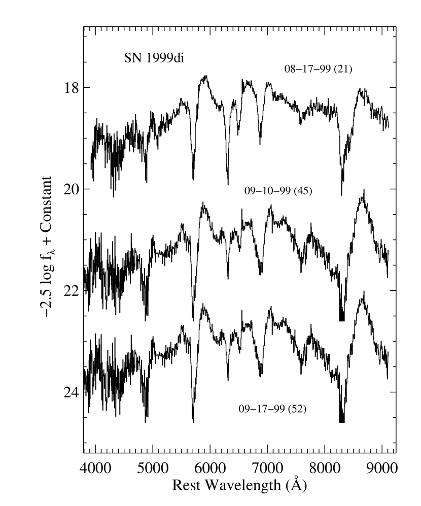
Figure 24: Spectra of SN Ib 1999di with flux units as in Figure 1. The following constants have been added to the individual spectra (from top to bottom): 0.0, 1.5, and 3.5. The recession velocity of the SN has been removed as described in the introduction to §3. The numbers after the date of observation indicate the approximate number of days past $R$-band maximum brightness based upon the light curve shown in Figure 27.

SN 1999di.—Puckett & Langoussis (1999) discovered SN 1999di on 1999 August 8 at magnitude 18 in NGC 776. The narrow (H II region) H$\alpha$ emission line in the spectra of SN 1999di indicates a recession velocity of 4920 km s^-1, effectively identical with the listed value for the host galaxy, NGC 776 (4921 km s^-1). Filippenko et al. (1999) classified it as a Type Ib. Spectra of SN 1999di (Figure 24) show the He I lines as well as a strong absorption at $\sim$ 6300 Å that may be Si II $\lambda$6355 or C II $\lambda$6580 (cf. §4.2). It is possible that this absorption is due to H$\alpha$, but the corresponding H$\beta$ line is not present.

SN 1999dn.—The BAO Supernova Survey found SN 1999dn on 1999 August 20 at a magnitude of 16 in NGC 7714 (Qiu, Qiao, & Hu 1999). The recession velocity of SN 1999dn is 2700 km s^-1, determined from the narrow (H II region) H$\alpha$ emission line. The listed velocity of NGC 7714 is 2799 km s^-1. There was confusion about the classification of this SN. While Ayani et al. (1999) and Turatto et al. (1999) described it as a Type Ic SN, Qiu et al. (1999) reported it as a Type Ia SN. The helium lines were visible (Pastorello et al. 1999), so it was also listed as a Type Ib/c SN. Our spectra (Figure 25) unambiguously indicate that it is a SN Ib. This was also the conclusion of Deng et al. (2000), who used a synthetic-spectrum code to model SN 1999dn. They also suggest that there is evidence for a weak hydrogen line, implying that SN 1999dn might have had an extremely low-mass hydrogen envelope.

SN 1999ec.—The LOSS discovered SN 1999ec on 1999 October 3 at magnitude 18 in NGC 2207 (Modjaz & Li 1999). Narrow (H II region) H$\alpha$ emission in the spectrum of SN 1999ec yields a recession velocity of 2800 km s^-1, while NGC 2207 has a listed velocity of 2746 km s^-1. It was classified as a SN Ib by Jha et al. (1999b), who described it as having prominent helium lines in a spectrum taken on 1999 October 5. Our single spectrum (obtained 1999 October 8, Figure 26) does not appear to fit obviously into any category. While there is an absorption line near 5700 Å, this could simply be Na I D alone, not Na I D and He I $\lambda$5876; note that the other helium lines are invisible. It could still be a SN Ib, but at late times. The [O I] $\lambda\lambda$6300, 6364 lines, however, are not present at their usual strength for a SN Ib. We believe that this is a peculiar SN I event, but the type is uncertain. It may be related to SN 1993R, an object that showed an unusual blend of SN Ib/c and SN Ia features (Filippenko & Matheson 1993; Matheson et al. 2001).

4 Discussion

To characterize our data on SNe Ib and SNe Ic, we will include comparisons with several of the best-observed examples of each class. One of the first well-studied SNe Ib was SN 1984L; we will use the data from Harkness et al. (1987). A late-time spectrum of SN Ib 1983N is taken from Gaskell et al. (1986). We will also use spectra of SN 1985F (Filippenko & Sargent 1986). As there was no spectrum of this SN near maximum light, the type is uncertain. The light curve (Filippenko et al. 1986; Tsvetkov 1986), however, is more consistent with those of SNe Ib than SNe Ic (Wheeler & Harkness 1990), and we will treat it as such. By far the most extensively studied SN Ic is SN 1994I; the spectra from Filippenko et al. (1995) will be used for comparison. In addition, we will consider the SN Ic 1987M (Filippenko, Porter, & Sargent 1990).

4.1 Evolution of SNe Ib

The set of spectra of SNe Ib in our sample is quite heterogeneous; there are few epochs for any given SN. For three of the SNe Ib, though, we have a light curve and can place the spectra relative to maximum light. The $R$-band and unfiltered-magnitude light curves of these three SNe are shown in Figure 27. The light curves for the individual SNe were shifted in time and magnitude to match one another with 0 mag indicating maximum brightness. The derived $R$-band maxima for the SNe are as follows: SN 1998dt, 1998 September 12; SN 1999di, 1999 July 27; SN 1999dn, 1999 August 31. Given the sparse nature of the points, an exact match was not possible. Shifting any one of the three curves by a day or two in either direction yields a similar result; thus, in all subsequent discussion of the relative phases of the spectra, an uncertainty of one or two days is appropriate. For the sake of completeness, we also show a partial light curve of the SN IIb 1998fa offset from the SNe Ib in Figure 27; its derived $R$-band maximum is 1999 January 2.

With the knowledge of the dates of the $R$-band maxima for the three SNe Ib, we can register the spectra and assign them a phase, as listed in Table 2. When these spectra are arranged in phase order (Figure 28), it is apparent that there is variation in the relative strengths of the He I P-Cygni absorptions. It is possible that this is just evidence of the differences among the SNe, but the variation seems to follow the temporal order even within the set of spectra for an individual object. There may be variations in the abundance of helium or the level of mixing, but we will ignore those effects for the present time to see whether changes in the helium lines do indicate a standard evolutionary behavior for the spectra of SNe Ib.

To make a comparison of the lines among different spectra, we had to develop a technique for characterizing the line strength. Traditional line-measuring methods are not applicable here. The equivalent width of the lines is dependent on a well-defined continuum, and this is not available as the spectra consist of a pseudo-continuum of many overlapping lines. We attempted to determine the line strength using local parameters for each line. We defined an “effective” equivalent width by setting a local continuum, integrating the flux in the line, and dividing by the value of the continuum. To do this, we chose relatively smooth regions on either side of the absorption to define the local continuum (Figure 29 illustrates the technique). The median value of each region was evaluated and a straight line fit through the two points (each point having the wavelength of the center of its continuum region and the flux of the median value). We then chose the edges of the line (generally where the continuum regions began, but with occasional subjective excursions). The flux within the line was evaluated in two ways. First, we summed the flux directly. Second, we fit a Gaussian to the line and summed the flux it represented. Both methods gave effectively the same results. As can be seen in Figure 29, the Gaussian fit the absorption rather well, although for some lines other than helium, it was more problematic. The “equivalent widths” determined with this technique did not yield any pattern indicating a temporal sequence for our spectra of SNe Ib. Complicating factors such as differing expansion velocity and placement of the continuum introduced a large uncertainty into each value.

Another possibility for measuring the lines came from considering only the depth of the line to eliminate some of the impacts from these potential sources of error. The depth was not dependent on the definition of the precise edges of the lines—the most subjective aspect of the measurement. One only had to find the minimum of the line, determine the flux of the spectrum at that point, evaluate the “continuum” flux at that wavelength from the line fit to the regions on either side of the absorption, and then use those fluxes to calculate the fractional line depth. The value for the line depth is measured from these fluxes using the formula

$${\rm{Fractional~{}Line~{}Depth}}=\frac{\it{F}_{\rm{cont}}-\it{F}_{\rm{min}}}{\it{F}_{\rm{cont}}},$$

where ${F_{\rm{cont}}}$ and ${F_{\rm{min}}}$ represent the flux values of the continuum and of the line minimum at the wavelength of the minimum, respectively. For noisy spectra, the region around the minimum was smoothed by a boxcar chosen to match approximately three times the spectral resolution. This smoothed subset determined the location and value for the minimum flux. The value of the fractional line depth thus gave a less subjective measurement for the scale of a given absorption. Larger values of the fractional line depth indicate a deeper and, presumably, stronger absorption. This is somewhat related to the technique used by Nugent et al. (1995) to estimate the strengths of absorptions in the spectra of SNe Ia, although their continuum was determined by two points, not a fit to a continuum region as we do.

We then took the line depths and normalized them to the fractional depth of the He I $\lambda$6678 line. In the SNe Ic, we still scaled to the feature closest to the expected position of this line, but, as discussed below, it is likely not the helium line. Thus, for each spectrum we have a fractional line depth scaled to a particular line. If there are helium abundance variations, then the normalization by the $\lambda$6678 line should help to lessen any impact. These values are listed in Table 3.

When the line depths for the SNe Ib that can be put in temporal order are compared, a pattern appears for the helium lines (see Figure 30). Both $\lambda$5876 (probably contaminated by Na I D) and $\lambda$7065 grow in strength relative to $\lambda$6678. The values are not exactly monotonic, but the trend is there within the scatter. The $\lambda$7281 line was either not present at great strength or too difficult to isolate in many of our spectra; for the ones in which it could be measured, a trend was not obvious.

To test this pattern, we examined two spectra of SN 1984L that have the three relevant He I lines. For the 1984 September 23 spectrum, the line ratios indicate that it is probably between our day 21 and day 38 spectra (see Figure 28). The date of maximum for SN 1984L is not well known, but $B$ maximum was approximately 1984 August 20 (August 20 $\pm$ 4, Tsvetkov 1985; Schlegel & Kirshner 1989). That puts this spectrum at day 34, modulo differences between $B$ and $R$ maximum, which falls within our (admittedly broad) window. The second spectrum (1984 September 29) fits in days 17-33, slightly earlier than the September 23 spectrum, so the scheme clearly is not complete. The first spectrum, though, could be day 21 and the second thus day 27, thereby still fitting within our model, although the date of maximum would have to be incorrect by almost two weeks, and that is not likely. If the September 29 spectrum is day 33, then the September 23 spectrum would be day 27 (consistent with our model’s predictions) and the date of maximum would be off by six days. As the date of maximum is estimated from later points on the light curve, this may be reasonable.

For SN 1991ar, the line-depth values for the 1991 September 16 spectrum indicate a phase of $21-38$ days, although this is more uncertain than most. The 1991 October 2 spectrum seems to be from a later phase, probably greater than 52 days. The 16 days between observations is consistent with our predicted ages. Discovery was on September 2, so it was at least 14 days past explosion by September 16 and 30 days past explosion by October 2. Our predicted ages are relative to the date of maximum brightness, so we would expect that the actual explosion date was much earlier than September 2. Phillips (1991b) called it “a few weeks old” on September 14, again consistent with our numbers.

The line-depth values for the 1997 September 6 spectrum of SN 1997dc are almost identical with those of the 1999 August 19 spectrum of SN 1999di. This would make its age about 21 days past maximum and most likely less than 33 days. Discovery was on 1997 August 5, with pre-discovery images confirming its presence on 1997 July 26 (see discussion of the individual SNe above). An explosion date near July 26 and a rise to maximum of approximately 15 days (cf. Figure 27) would make Sept 6 roughly 27 days past $R$-band maximum. Within the uncertainty of our age estimates, this is consistent.

The model does not work at all with the values measured from SN 1998T. Considering only the $\lambda$5876 line, both the 1998 March 6 and March 27 spectra fit in the $21-38$ day range. Discovery was on March 3 (Li et al. 1998a), but the March 6 spectrum is evidently older than just a few days past maximum (compare with the early spectra of SN 1984L in Harkness et al. 1987). This SN is superposed on an extremely bright H II region, and contamination from the narrow H$\alpha$ line made measurements of the $\lambda$6678 line problematic. In addition, while the ratios of the line depths are consistent with those of other SNe Ib, the scale of the fractional line depth of the individual lines was much less. As can be seen in Figure 20, the spectra are very blue, indicating a high level of starlight contamination. It is possible that the combination of measurement errors and dilution render our line-depth values useless in this case. SN 1998T is a clear exception to the otherwise high level of homogeneity among SNe Ib.

When we try to determine the relative ages of the seven spectra of SNe Ib (SNe 1984L, 1991ar, 1997dc, and 1998T) that were not used to develop the pattern of helium-line depths, the result is not completely successful. Figure 28 shows the training set of spectra in the proper order with the six test spectra inserted in the approximately correct positions. The spectra of SN 1984L fit to a certain degree, but the 1984 September 29 spectrum does not quite match the model. SN 1991ar and SN 1997dc seem to work well, although it is difficult to be certain with only a single spectrum for SN 1997dc. The results with SN 1998T are in conflict with the model. The apparent contamination in the spectra may be the cause of this problem, but it may also indicate that there is not a simple sequence of temporal evolution of the helium lines for SNe Ib or that helium-line strength is intrinsically variable. The rest of the SNe Ib in the sample, however, are remarkably homogeneous.

4.2 Helium Lines in SNe Ib and SNe Ic?

One other result of the line-fitting technique is that the expansion velocity of the minimum of the line is measured along with an estimate of the velocity width of the absorption. These values are listed in Table 4. The SNe Ib all have fairly consistent expansion velocities in the range $7000-9500$ km s^-1. The SNe Ic have similar velocities for the line referred to as He I $\lambda$5876, but this is probably Na I D. The line referred to as He I $\lambda$6678, though, has fairly large values ($16100-18900$ km s^-1, with one at 12200 km s^-1) for the SNe Ic—so large that this line is probably not helium, but rather some other species that appears in most SNe Ic.

Clocchiatti et al. (1996) claim that helium lines, including $\lambda$5876 and $\lambda$6678, are present in the spectra of many SNe Ic at a high velocity. (Munari et al. [1998] made similar claims for SN 1997X, but inspection of their spectra indicates that this is a less certain identification.) Figure 31 shows two of the SNe that Clocchiatti et al. (1996) considered (SNe 1994I and 1987M) along with several SNe Ic in our sample and a SN Ib for comparison. The expected positions of the He I lines at expansion velocities of $-15000$ to $-19000$ km s^-1 are marked. For SNe 1994I and 1987M, a broad feature is at the expected location of high-velocity He I $\lambda$6678, as well as a narrower line at the expected high-velocity position of He I $\lambda$5876. The other helium lines may appear in SNe 1994I and 1987M, but they are weak. The other SNe Ic from our sample do not seem to exhibit this same pattern, although, as mentioned above, in the 1991 January 17 spectrum, SN 1991A does have a double-minimum structure between 5300 Å and 5800 Å that may be Na I D and high-velocity He I $\lambda$5876. There is a feature near 6300 Å in some of the SNe Ic that would match the He I $\lambda$6678 line, but the other lines are not there. If anything, SN 1990B seems to show weak low-velocity helium lines that match the SN Ib, although this identification is tentative.

It may be that the small features Clocchiatti et al. (1996) interpreted as high-velocity helium are actually other species at low velocities. The small dip near 5550 Å that they claimed as high-velocity He I $\lambda$5876 also appears in the spectrum of the SN Ib 1999dn as a shoulder on the blue edge of the He I $\lambda$5876 + Na I D line, but the SN Ib does not have any unexpected features at the locations of the other high-velocity helium lines (the low-velocity position of He I $\lambda$7065 is coincident with the high-velocity position of He I $\lambda$7281 for SN 1999dn).

The identification of the line that appears near 6300 Å remains uncertain. Millard et al. (2000) suggested C II $\lambda$6580 was present in SN 1994I at a high, detached velocity of 16000 km s^-1. (Deng et al. [2000] come to similar conclusions for the SN Ib 1999dn.) This line would still have a fairly high velocity ($12000-13000$ km s^-1) in our spectra, but seems more likely than helium. As discussed below, carbon and oxygen lines might stand out more in SN Ic spectra because they are not diluted by a helium layer as they would be in spectra of SNe Ib. It would be at a very low velocity if the line were Si II $\lambda$6355, but that remains a possibility. Careful spectral synthesis modeling may be able to finalize the identification of this line.

Clocchiatti et al. (1996) found that there was not a continuum of helium-line strength that would imply a gradual transition from SNe Ib to SNe Ic. This is also apparent from our spectra, especially in light of the uncertain line near 6300 Å. For all of the objects listed in Tables 3 and 4, if helium lines are present, then they are distinct in the spectra. The SNe Ib shown in Figure 28 all have fairly similar helium-line strengths, except for SN 1998T. It, though, appears to suffer a high level of contamination that is diluting the helium lines. In fact, the SNe Ib in Figure 28 are similar overall, except for the appearance of the 6300 Å line in SN 1999di (see Deng et al. 2000 for a further discussion of such lines in a SN Ib).

Other claims of detection of helium in SNe Ic have been put forth. Filippenko et al. (1995) showed an apparent P-Cygni profile of He I $\lambda$10830 (a minimum at $\sim$ 10250 Å) in SN 1994I. The $\lambda$10830 line, though, should be much stronger than the other optical helium lines (Swartz et al. 1993b) and can be produced with very small amounts of helium (Wheeler, Swartz, & Harkness 1993; Baron et al. 1996). Therefore, the He I $\lambda$10830 line could be present without requiring evidence for the other optical helium lines. More detailed spectral synthesis models indicate that even the $\lambda$10830 identification may be questionable (Baron et al. 1999; Millard et al. 1999). These models have found that C I (multiplet 1, $\lambda$10695) and Si I multiplets 4 ($\lambda$12047), 5 ($\lambda$10790), 6 ($\lambda$10482), and 13 ($\lambda$10869) may contribute to the near-IR feature observed in SN 1994I. In fact, Si I may contribute near 7000 Å, explaining the features seen there in some SNe Ic (Millard et al. 1999). The SN Ic 1999cq showed intermediate-width helium emission lines in its spectra, but these were more likely the result of an interaction with circumstellar material, not evidence for helium in the ejecta of the SN itself (Matheson et al. 2000b).

It may be that the transition objects between SNe Ib and SNe Ic are rare or have been overlooked. For example, only a few objects have been observed in the SN IIb class out of the hundreds of normal SNe II and SNe Ib. If this ratio holds for the SNe Ib with weak helium, then perhaps an object bridging SNe Ib and SNe Ic has been missed. Weak lines in some SNe Ic are at the wrong positions to be helium, unless the velocities are very large, and then only a subset of the lines appears. It is possible that the lines in SNe 1987M and 1994I are helium, but the rest of our SN Ic spectra do not show the same patterns. If this is the case, then SNe 1987M and 1994I (and, perhaps, 1990B) are the transition objects between SNe Ib and Ic, while the true Type Ic SNe show no helium at all, with the possible exception of He I $\lambda$10830.

In addition to the controversy over the presence of helium, there have been some claims of hydrogen in SNe Ic. Jeffery et al. (1991) suggested that there was evidence for hydrogen in the spectra of SN 1987M. Filippenko (1992) concurred on SN 1987M, as well as claiming that SN 1991A (and perhaps SN 1990aa) also revealed weak hydrogen lines. If some SNe Ic do retain enough hydrogen to produce observable lines, then it is likely that there is helium present as well. In this scenario, mixing of radioactive nickel into a helium layer would be the more important factor in determining whether or not helium lines appear. As discussed below, though, the SNe Ic in general seem to have less massive envelopes than the SNe Ib. If that is the case, the presence of hydrogen in the spectra of SNe Ic is quite mysterious, although mixing at earlier phases in the star’s evolution may have introduced hydrogen into the carbon-oxygen or (low-mass) helium layer of the star. Detailed spectral modeling may indicate if this identification is correct.

4.3 Spectroscopic Distinction of SNe Ib and SNe Ic

4.3.1 Expansion Velocity from Late-Time Spectra

If the difference between progenitors of SNe Ib and SNe Ic is due to the absence (or at least partial absence) of a helium envelope in the latter, then it may be possible to see an impact of this in the late-time, nebular-phase spectra as well as at early times. For a given input energy, a lower-mass envelope will be expelled with a higher velocity. The apparent increase in velocity width from Types II through IIb, Ib, and Ic may indicate a decreasing envelope mass (Figure 32). Whether or not the explosion energy is the same for all core-collapse events is questionable, but we will assume that it does not vary much for the purposes of this analysis.

In a study of late-time spectra of SNe Ib, Schlegel & Kirshner (1989) found the velocity widths of [O I] $\lambda\lambda$6300, 6364 and [Ca II] $\lambda\lambda$7291, 7324 to be FWHM = 4500 $\pm$ 600 km s^-1. Filippenko et al. (1995) determined larger values for two SNe Ic (SN 1994I, FWHM = 7700 km s^-1 for [O I] and FWHM = 9200 km s^-1 for [Ca II]; SN 1987M, FWHM = 7500 km s^-1 for [O I] and FWHM = 6200 km s^-1 for [Ca II]). They interpreted this as evidence for smaller envelope mass and/or larger explosion energy in SNe Ic compared with SNe Ib.

We measured the velocity width of nebular emission lines with a Gaussian fit to the line after a continuum fit to the spectrum by hand had been subtracted. The continuum placement was subjective, but the late-time spectra are simple and have fairly well-defined continua; errors in the location of the continuum have little impact on the value of the FWHM of the fit line. The subset of our data with measurable nebular-phase emission lines (along with SNe 1983N, 1985F, 1987M, and 1994I) are listed in Table 5 with the values from the Gaussian fit for the FWHM of the lines.

Unfortunately, despite the large number of SNe Ib in our sample, none of them is at a sufficiently late stage to provide clean, nebular emission lines. For the SNe Ib, we will rely on the values of Schlegel & Kirshner (1989) and the SN Ib 1983N. There are many good examples of late-time SNe Ic spectra. Not all of the spectra are useful though. The values for SN Ic 1995F are very large. The lines appear to be contaminated (on the blue edge of [O I] $\lambda\lambda$6300, 6364 and red edge of [Ca II] $\lambda\lambda$7319, 7324—cf. Figure 12), and we will not use it in the determination of the mean values. SNe Ic 1997dq and 1997ef seem to be spectroscopically peculiar (discussed below), and thus will not be included for a general estimate of the velocity widths of later-time SN Ic emission lines either. We also exclude SN 1991aj and SN 1995bb, as their exact classification is uncertain. The velocities of the lines for these two SNe are very similar to the range listed for the other SNe Ic, and are clearly less than the average Schlegel & Kirshner (1989) reported for SNe Ib, but without a definite type, they should not be used. Adding them to the SN Ic set of velocities, though, does not alter the values reported below significantly. Note that we do include SNe Ic 1994I and 1987M. Our values for [O I] $\lambda\lambda$6300, 6364 and [Ca II] $\lambda\lambda$7319 for the 1994 September 2 spectrum of SN 1994I and the 1988 February 25 spectrum of SN 1987M are virtually identical to the numbers reported by Filippenko et al. (1995), despite using slightly different techniques to determine the line widths.

For each of the relatively normal SNe that remains, we will consider only the latest possible value for any given line. To calculate the mean value for the emission lines, each SN will contribute one number; otherwise, a single SN with spectroscopic coverage over many late epochs could bias the mean value. In this way the heterogeneity of the SNe Ic is reflected in the computed standard deviation. For [O I] $\lambda\lambda$6300, 6364, the mean velocity width for Type Ic SNe is 7600 $\pm$ 2100 km s^-1 (median = 7300 km s^-1) with nine data points. The mean is 8700 $\pm$ 2700 km s^-1 (median = 8500 km s^-1) for [Ca II] $\lambda\lambda$7319, 7324 with eight data points. Combining both [O I] $\lambda\lambda$6300, 6364 and [Ca II] $\lambda\lambda$7319, 7324 as has been done with the Schlegel & Kirshner (1989) data for SNe Ib, the mean velocity width is 8100 $\pm$ 2400 km s^-1 (median 7400 km s^-1).

The calcium near-IR triplet is more problematic to measure than the other lines discussed. As it has three components, the line profile is not as Gaussian-shaped as it is for [O I] $\lambda\lambda$6300, 6364 and [Ca II] $\lambda\lambda$7319, 7324 and the total width of the line does not represent only the expansion velocity. The intrinsic width of the near-IR triplet in velocity space is $\sim$ 5700 km s^-1, significantly larger than the velocity separation of the two [O I] components of $\sim$ 3000 km s^-1. With these caveats, the mean value for the near-IR triplet must be viewed with caution. The velocity width for the triplet in SNe Ic is 10800 $\pm$ 1600 km s^-1 (median = 10800 km s^-1) with eight points contributing. Table 5 also lists O I $\lambda$7774, but this line is not present in many of the spectra and its mean value is not reliable.

Table 5 also lists values for two SNe Ib (1983N and 1985F). The average of these two for the [O I] $\lambda\lambda$6300, 6364 lines is 5600 km s^-1 while it is 5200 km s^-1 for [Ca II] $\lambda\lambda$7319, 7324 (standard deviations for only two measurements are not meaningful and are not reported). When both lines are considered together, the mean velocity width is 5400 $\pm$ 300 km s^-1. With only two points, the mean values are much less certain. SN 1985F was part of the Schlegel & Kirshner (1989) data set. If we combine the numbers from Schlegel & Kirshner (1989) for SNe 1984L, 1985F, and 1987K with our values for SN 1983N (considering only the latest possible value for each line in each SN), the mean velocity width of [O I] $\lambda\lambda$6300, 6364 and [Ca II] $\lambda\lambda$7319, 7324 for SNe Ib is 4900 $\pm$ 800 km s^-1. As mentioned above, [O I] $\lambda$6300 and [O I] $\lambda$6364 are separated by $\sim$ 3000 km s^-1. This blending may artificially broaden the line as measured, yield exaggerated expansion velocities. The values for [O I] $\lambda\lambda$6300, 6364 in Table 5, however, are comparable to those of [Ca II] $\lambda\lambda$7319, 7324, whose two components are just $\sim$ 200 km s^-1 apart. This implies that $\lambda$6300 dominates the flux of doublet and the velocity as measured is a good indication of the actual expansion.

The lines of [O I] $\lambda\lambda$6300, 6364 and [Ca II] $\lambda\lambda$7319, 7324 at late times are fairly representative of the velocity width of the expansion. All of the measurements for SNe Ic in Table 5 are larger than the mean value for SNe Ib. Only SN Ic 1990U has a velocity width approaching that of the SNe Ib. A Kolmogorov-Smirnov (KS) test indicates that the distributions of line widths for SNe Ib and SNe Ic are different at the 99% confidence level.

It seems unlikely that every SN Ic has a higher explosion energy than SNe Ib. Thus, the more probable cause is that the SNe Ic have lower-mass envelopes, lending credence to the argument that the progenitors of SNe Ic have lost most or all of their helium layer. If a lack of mixing were the sole reason that SNe Ic do not show helium lines, then one would expect that the envelope masses of SNe Ib and SNe Ic would be comparable. It may be that mixing still plays a role, but the velocity widths of the late-time emission lines indicate that there appears to be a distinct difference between the envelope masses for SNe Ib and Ic.

4.3.2 Permitted Oxygen Lines

Another test of the lost-envelope scheme for producing SNe Ic is to examine a feature that might appear more prominently if the helium were removed. A massive star that has lost its hydrogen and helium (or at least most of the helium) would be left with a carbon-oxygen core. This new envelope could produce lines of carbon or oxygen at relatively greater strength than could one in which those species are diluted by the presence of a large amount of helium (or hydrogen). If this is the case for SNe Ic, then the oxygen lines present in their spectra might appear to be relatively stronger than they do in the spectra of SNe Ib.

To test this hypothesis, we chose to study the O I $\lambda$7774 line. It is in a region of the spectrum that is relatively uncontaminated by other lines and is readily accessible in most of our spectra (unlike O I $\lambda$9266). Figure 33 illustrates the apparent increase of O I $\lambda$7774 line strength from Types II through IIb, Ib, and Ic. This increase could be the result of decreasing envelope mass. In each of our spectra that contained a relatively distinct P-Cygni profile of O I $\lambda$7774, we employed our fractional line depth technique described above in §4.1. The results are listed in Table 6. For this discussion, we will not include the values for the peculiar SN Ic 1997dq. The fractional line depth of the oxygen line is the most useful of the measurements listed. The velocity at the minimum of the P-Cygni absorption is probably fairly accurate, but the velocity width of the absorption measured by the fit Gaussian is not particularly representative. Unlike the He I lines discussed above, the Gaussian did not appear to match the profile very well; we report the number for completeness.

The mean value for the line depth for all measurements of SNe Ib is 0.27 $\pm$ 0.11 (median = 0.25) while that for SNe Ic is 0.38 $\pm$ 0.091 (median = 0.37). If we consider only the values from the earliest possible spectrum for each SN (i.e., only counting one value for each SN, where we are examining the outermost layers of the expanding ejecta), the mean for SNe Ib becomes 0.22 $\pm$ 0.10 (median = 0.20) and that of the SNe Ic becomes 0.41 $\pm$ 0.099 (median = 0.39). To see if there is a difference between the values for the SNe Ib and SNe Ic, we compared them using a KS test. The KS test indicates that the two distributions (O I line depths for SNe Ib and Ic) are different at a confidence level of 97%. The differences suggest that the SNe Ic do have a relatively stronger O I $\lambda$7774 line, implying that they may have a lower-mass (or even non-existent) helium envelope overlying the oxygen layer of their progenitors.

The expansion velocity implied by the minimum of the O I $\lambda$7774 line is slightly larger for SNe Ic than for SNe Ib (mean of 6900 km s^-1 for SNe Ib vs. 8300 km s^-1 for SNe Ic). This is consistent with the results described above for the nebular-phase line widths, but the difference is smaller and probably less significant. The minimum for the O I $\lambda$7774 line was more difficult to define than for the helium lines due to its generally broader shape and its position on a changing part of the overall spectral profile.

4.4 Are the SNe Ic a Uniform Class?

Aside from SN 1998T, the spectra of the SNe Ib in Figure 28 are all fairly similar. What about the SNe Ic? There are measured light curves for two of the SNe Ic in our sample, SN 1990B (Clocchiatti et al. 2001) and SN 1990U (Richmond, Filippenko, & Galisky 1998). Combining these (and ignoring for now the possibility of two different types of light curves for SNe Ic [Clocchiatti et al. 1997; see below]), we can define the time of maximum light for SN 1990B and SN 1990U and register the two sets of spectra to a common phase (Figure 34). For the case of the SNe Ib, the relative strengths of the helium lines provided a possible indicator for the relative age of the SNe. Unfortunately, there is not a comparable measurement that shows the evolution of the SNe Ic.

Despite the lack of phase information, the spectra of SNe Ic in our sample do allow some generalizations to be made. One of the spectroscopic differences among the various objects is the relative smoothness of the spectrum in the range $6000-7500$ Å. For some SNe, P-Cygni profiles appear with absorption minima near 6300 Å and/or 6800 Å. The apparent He I $\lambda$7065 minimum is often near 6800 Å, but the 6300 Å line is probably not helium (see discussion above). The point is that some SNe Ic have one or both of these features, and the others do not. Considering only the relatively normal SNe Ic that have spectra during the photospheric phase (or at least show some photospheric features), we have three SNe Ic that are relatively smooth in this region (SNe 1991A, 1991N, and 1994I) and five that show many distinct lines between $6000-7500$ Å (SNe 1988L, 1990B, 1990U, 1990aa, and 1995F).

The expansion velocities from the late-time nebular line velocity widths listed in Table 5 can be compared for the two subsets of SNe Ic. There is no correlation. The two lowest-velocity SNe are SN 1990U and SN 1991N, yet their spectra do not look very similar. In fact, the spectra of SN 1991N and SN 1994I do look similar, but they have disparate line widths.

Clocchiatti et al. (1997; see also Clocchiatti & Wheeler 1997) introduced a light-curve element into the classification of the SNe Ic. They found that there are two types of light curves, “fast” and “slow.” The light curve of SN 1990B is in the “slow” class (Clocchiatti et al. 2001). The comparison of this light curve with that of SN 1990U (Richmond et al. 1998) shows that SN 1990U also has a “slow” light curve. The only other SN Ic in our sample with a measured light curve is SN 1994I (e.g., Richmond et al. 1996); it is in the “fast” class. As mentioned above, there do appear to be some spectroscopic differences between SN 1994I and the two “slow” examples, SNe 1990B and 1990U. The speed of the light curve is apparently related to the overall mass of the ejecta, implying that SN 1994I had a smaller-mass envelope than did SN 1990B or SN 1990U. SN 1990U had narrower nebular-phase emission lines than SN 1994I (cf. Table 5), but SN 1990B was comparable to SN 1994I. Without a larger number of examples of the “fast” and “slow” classes having spectroscopic coverage, it is not clear if any correlation exists.

There does not appear to be a method for subclassifying our spectra of SNe Ic in a simple scheme. The class as a whole is distinct from the SNe Ib (and SNe II and SNe Ia), but further subdivision seems unwarranted at this time. Within the definable type of SN Ic, though, there is a substantial level of heterogeneity.

4.5 The Peculiar SNe Ic 1997dq and 1997ef

The possible association of the peculiar SN Ic 1998bw with gamma-ray burst (GRB) 980425 (e.g., Galama et al. 1998; Iwamoto et al. 1998; Woosley, Eastman, & Schmidt 1999) has helped to fuel a flurry of work postulating that the GRBs are the result of some form of stellar collapse (see, e.g., MacFadyen & Woosley 1999; Nomoto et al. 2000; Wheeler 2000; Lamb 2000, and references therein). The temporal appearance and location of SN 1998bw were approximately coincident with GRB 980425. The optical luminosity was significantly larger than in a typical SN Ic (e.g., Galama et al. 1998; Iwamoto et al. 1998; Woosley, Eastman, & Schmidt 1999; for a comparison with other GRBs and SNe, see Bloom et al. 1998). Moreover, radio observations exhibited a prompt turn-on and provided evidence of relativistic motions (Kulkarni et al. 1998). Finally, the spectral features were broader than normal (see Nomoto et al. 2000; Kulkarni et al. 1998), indicating a smaller mass and/or higher explosion energy. SN 1997ef (cf. Figure 18) also had broader than usual emission and absorption features, causing Nomoto et al. (1999) to consider it in the same class as SN 1998bw (see also Nomoto et al. 2000; Iwamoto et al. 2000). It was also possibly associated with a GRB (971115, Wang & Wheeler 1998).

The late-time spectra of SN 1997dq and SN 1997ef appear quite similar (Figure 35), but the early-time spectra of SN 1997dq do not show lines as broad as those in SN 1997ef. This probably just reflects the lack of sufficiently early spectra for SN 1997dq. The GRB 971013 may be associated with SN 1997dq (Wang & Wheeler 1998), so it is possible that these two objects do represent a different class than the normal SNe Ic presented above. They may be examples of the “hypernovae” (Nomoto et al. 2000; Iwamoto et al. 2000) or “collapsars” (MacFadyen & Woosley 1999) that are postulated as the sources of GRBs. Another SN in our sample, SN 1997ei, may also be associated with a GRB (971120, Kippen et al. 1998; Wang & Wheeler 1998), but its spectra do not seem especially unusual (cf. Figures 19 and 35). We do not know the relative phases of all of our spectra, but none of our SN 1997dq or SN 1997ef spectra (which cover months of evolution) is a match for either of the spectra of SN 1997ei. Of course, apparent coincidental association between SNe and GRBs is insufficient evidence for a direct link between the objects. On the other hand, if SN 1997ei and GRB 971120 are indeed physically linked, this may imply that the GRBs that are also observed as SNe are a heterogeneous lot. Models that produce them must be able to account for the SNe 1998bw, 1997dq, and 1997ef types as well as the more normal-looking SN 1997ei.

5 Conclusions

We present 84 spectra of SNe Ib, Ic, and IIb, as well as $R$-band and unfiltered-magnitude light curves for three SNe Ib and one SN IIb. We find that three SNe in our sample that had originally been classified as SNe Ib/c (SNe 1991K, 1997C, and 1999bv) have spectra that are more consistent with those of late-time SNe Ia. An examination of the fractional depths of the helium lines in the SNe Ib reveals an apparent progression of relative line strengths as the SN evolved. The training set of SNe Ib for which we have light curves provides a model for the development of the helium lines. Other SNe Ib are fit into the sequence of ages as determined by their helium-line strengths, but with only partial success. Examination of all the SNe Ib spectra, though, does indicate that the SNe Ib have fairly consistent helium-line strengths. There are no clear examples of weak, but distinct, helium lines in the SNe Ib.

In considering the possible presence of helium lines in SNe Ic, we come to a different conclusion than Clocchiatti et al. (1996). They claim that spectra of various SNe Ic show helium lines at high velocity. The helium lines may be present in some of the objects that Clocchiatti et al. (1996) studied, but the SNe Ic in our sample show no consistent pattern of high-velocity helium lines. Other lines, such as C II $\lambda$6580, may explain the features of the SN Ic spectra. SN 1990B does appear to show some weak helium lines, but at low velocity. This may represent the transition between SNe Ib and SNe Ic, but the lines are not definitive.

We demonstrate other methods for distinguishing SNe Ib and SNe Ic spectroscopically. The emission lines in late-time, nebular-phase spectra of SNe Ic have average line widths (FWHM) of 8100 $\pm$ 2400 km s^-1, while incorporating the data of Schlegel & Kirshner (1989) gives a mean value of 4900 $\pm$ 800 km s^-1 for the SNe Ib. They are distinctly different, with the SNe Ic having clearly higher expansion velocities. Unless the SNe Ic have consistently higher explosion energies, this implies that SNe Ib have larger envelope masses in general than do SNe Ic.

Another indicator of the difference between SNe Ib and SNe Ic is the strength of the O I $\lambda$7774 line. If SNe Ic have had their helium envelopes removed, then the exposed oxygen core could yield relatively stronger lines as they are no longer diluted by the helium. We find that our fractional line depth measurements show the SNe Ic to have stronger O I lines (0.41 vs. 0.22 for SNe Ib). The KS test suggests that the difference between the SNe Ic and SNe Ib is real, once again implying that the SNe Ic do have smaller envelope masses than the SNe Ib.

Within the SN Ic class, there is a substantial heterogeneity. We can separate our SN Ic spectra into two classes based on the relative smoothness in the range $6000-7500$ Å, but the distinction is not definitive. In addition, no correlations with other line measurements are found. These two subsets may be related to the “fast” and “slow” photometric classes for SNe Ic that are described by Clocchiatti et al. (1997), but, with only limited examples, this is highly speculative. While it is apparent from our results discussed above that SNe Ic are distinct from SNe Ib (as well as from SNe II and SNe Ia), there is no obvious method yet for spectroscopically subclassifying them.

Finally, we explore two peculiar SNe Ic, 1997dq and 1997ef. Both of these SNe are possibly associated with GRBs. SN 1997ef has extremely broad emission lines at early times and has been modeled as a “hypernova” (e.g., Iwamoto et al. 2000). Features in early-time spectra of SN 1997dq are not as broad, but our temporal sampling is sparse. Later spectra of SN 1997dq match very well those of SN 1997ef, implying that it, too, is unusual in the same way as SN 1997ef. SN 1997ei also may be positionally and temporally coincident with a GRB, yet its spectra seem fairly normal for a SN Ic and do not resemble SNe 1997dq or 1997ef at any phase. It could be that the GRB association with SN 1997ei is incorrect (as may be the case for all of them), but if correct, then the models of “hypernovae” and “collapsars” must be able to produce typical SNe Ic such as SN 1997ei as well as the peculiar SN 1997ef.

The spectra presented in this paper, as well as the spectra of SN 1993J published by Matheson et al. (2000a), are available for analysis by other researchers. Please contact A.V.F. or T.M. if interested.

Figure 1: Spectra of SN Ib/c 1988L; see also Filippenko (1988). The flux units are $-2.5$ log $f_{\lambda}-21.10$, following the definition of Space Telescope (ST) magnitudes (e.g., Koorneef et al. 1986). ST magnitudes are analogous to AB magnitudes ($-2.5$ log $f_{\nu}-48.60$; Oke & Gunn 1983), with the zero point yielding monochromatic magnitudes for Vega in the Johnson $B,V,$ and $R$ passbands of $\sim$ 0. For clarity, the following constants have been added to the individual spectra (from top to bottom): 0.0, 1.0, 3.0, and 6.0. The recession velocity of the SN has been removed as described in the introduction to §3.

Figure 2: Spectra of SN Ic 1990B with flux units as in Figure 1; see also Clocchiatti et al. (2001). The following constants have been added to the individual spectra (from top to bottom): $-$2.0, $-$1.0, 1.5, 3.5, 4.5, 6.0, and 8.0. The recession velocity of the SN has been removed as described in the introduction to §3. The numbers after the date of observation indicate the approximate number of days past $R$-band maximum brightness based upon the light curve of Clocchiatti et al. (2001).

Figure 3: Spectra of SN Ic 1990U with flux units as in Figure 1. The following constants have been added to the individual spectra (from top to bottom): $-$1.0, 0.0, 0.5, 1.5, 4.0, 4.0, 7.0, 9.0, 11.0, and 12.5. The recession velocity of the SN has been removed as described in the introduction to §3. The numbers after the date of observation indicate the approximate number of days past $R$-band maximum brightness based upon the light curve of Richmond, Filippenko, & Galisky (1998). As the light curve for SN 1990U does not contain points near maximum brightness, it was temporally matched with the light curve for SN 1990B (Clocchiatti et al. 2001) to estimate the date of maximum.

Figure 4: Spectra of SN Ic 1990aa with flux units as in Figure 1; see also Filippenko (1992). The following constants have been added to the individual spectra (from top to bottom): 0.0, 1.5, 2.5, and 4.0. The recession velocity of the SN has been removed as described in the introduction to §3.

Figure 5: Spectrum of SN Ib/c 1990aj with flux units as in Figure 1. The recession velocity of the SN has been removed as described in the introduction to §3.

Figure 6: Spectra of SN Ic 1991A with flux units as in Figure 1; see also Filippenko (1992). The following constants have been added to the individual spectra (from top to bottom): $-$1.0, 0.5, 2.0, 3.5, 5.5, and 8.0. The recession velocity of the SN has been removed as described in the introduction to §3.

Figure 7: Spectra of SN Ib 1991D with flux units as in Figure 1. The following constants have been added to the individual spectra (from top to bottom): $-$1.0, 0.0, and 1.0. The recession velocity of the SN has been removed as described in the introduction to §3.

Figure 8: Spectra of SN 1991K, SN 1997C, SN 1999bv, the Type Ia SN 1994D, the peculiar Type Ia SN 1991bg (Filippenko et al. 1992b), and the Type Ic SN 1994I with flux units as in Figure 1, offset by arbitrary amounts. The recession velocities of the SNe have been removed as described in the introduction to §3. Note the similarity of SN 1991K and SN 1999bv to SN 1994D, especially the day 87 spectrum. They do not seem to match the spectrum of SN 1994I (at any phase, cf. Filippenko et al. 1995). SN 1997C is also similar to SN 1994D, but shares more characteristics with the spectrum of the sub-luminous Type Ia SN 1991bg. We believe this indicates that SN 1991K, SN 1997C, and SN 1999bv were originally misclassified and were actually SNe Ia caught past maximum. Without spectra near maximum brightness, though, there is still some uncertainty.

Figure 9: Spectrum of SN Ib/c 1991L with flux units as in Figure 1. The recession velocity of the SN has been removed as described in the introduction to §3.

Figure 10: Spectra of SN Ic 1991N with flux units as in Figure 1. The continuum is heavily contaminated by superposed stars; the strong, narrow emission lines are from a superposed H II region. An apparent calibration error affects the red half of the 1992 January 9 spectrum. The following constants have been added to the individual spectra (from top to bottom): 0.0, 1.5, 3.0, 5.5, and 8.0. The recession velocity of the SN has been removed as described in the introduction to §3.

Figure 11: Spectra of SN Ib 1991ar with flux units as in Figure 1. The following constants have been added to the individual spectra (from top to bottom): 0.0 and 1.0. The recession velocity of the SN has been removed as described in the introduction to §3.

Figure 12: Spectra of SN Ic 1995F with flux units as in Figure 1. The following constants have been added to the individual spectra (from top to bottom): 0.0, 1.8, 3.0, and 5.0. The recession velocity of the SN has been removed as described in the introduction to §3.

Figure 13: Spectrum of SN Ib/c 1995bb with flux units as in Figure 1. The recession velocity of the SN has been removed as described in the introduction to §3.

Figure 14: Spectra of SN IIb 1996cb with flux units as in Figure 1. The following constants have been added to the individual spectra (from top to bottom): 0.0, 1.3, and 2.5. The recession velocity of the SN has been removed as described in the introduction to §3.

Figure 15: Spectrum of SN Ib 1997dc with flux units as in Figure 1. The recession velocity of the SN has been removed as described in the introduction to §3.

Figure 16: Spectrum of SN IIb 1997dd with flux units as in Figure 1. The recession velocity of the SN has been removed as described in the introduction to §3.

Figure 17: Spectra of SN Ic 1997dq with flux units as in Figure 1. The following constants have been added to the individual spectra (from top to bottom): $-$4.0, $-$2.0, 8.0, 1.8, and 3.0. The recession velocity of the SN has been removed as described in the introduction to §3.

Figure 18: Spectra of SN Ic 1997ef with flux units as in Figure 1. The following constants have been added to the individual spectra (from top to bottom): 0.0, $-$0.5, 1.5, 3.0, 6.0, and 7.5. The recession velocity of the SN has been removed as described in the introduction to §3. The numbers after the date of observation indicate the approximate number of days past $V$-band maximum brightness based upon the light curve of Iwamoto et al. (2000).

Figure 19: Spectra of SN Ic 1997ei with flux units as in Figure 1. The following constants have been added to the individual spectra (from top to bottom): 0.0 and 0.5. The recession velocity of the SN has been removed as described in the introduction to §3.

Figure 20: Spectra of SN Ib 1998T with flux units as in Figure 1. The following constants have been added to the individual spectra (from top to bottom): 0.0 and 1.3. The recession velocity of the SN has been removed as described in the introduction to §3.

Figure 21: Spectra of SN Ib 1998dt with flux units as in Figure 1. The following constants have been added to the individual spectra (from top to bottom): 0.0 and 1.0. The recession velocity of the SN has been removed as described in the introduction to §3. The numbers after the date of observation indicate the approximate number of days past $R$-band maximum brightness based upon the light curve shown in Figure 27.

Figure 22: Spectra of SN IIb 1998fa with flux units as in Figure 1. The following constants have been added to the individual spectra (from top to bottom): 0.0, 1.8, 3.0, and 6.0. The recession velocity of the SN has been removed as described in the introduction to §3.

Figure 23: Spectrum of SN Ib/c 1999P with flux units as in Figure 1. The recession velocity of the SN has been removed as described in the introduction to §3.

Figure 25: Spectra of SN Ib 1999dn with flux units as in Figure 1. The following constants have been added to the individual spectra (from top to bottom): $-$2.0, 0.0, and 1.5. The recession velocity of the SN has been removed as described in the introduction to §3. The numbers after the date of observation indicate the approximate number of days past $R$-band maximum brightness based upon the light curve shown in Figure 27.

Figure 26: Spectrum of SN Ib/c(?) 1999ec with flux units as in Figure 1. The recession velocity of the SN has been removed as described in the introduction to §3.

Figure 27: KAIT $R$-band and unfiltered-magnitude light curves of the SNe Ib 1998dt (circles), 1999di (triangles), and 1999dn (squares), along with the SN IIb 1998fa (stars). True $R$-band values are indicated by solid symbols; unfiltered magnitudes are shown as open symbols. As described in §2, unfiltered magnitudes for KAIT are similar to $R$-band values. The points have been shifted arbitrarily in magnitude to yield 0 at maximum (SN 1998fa is offset by $-1.5$ mag). The arrow on the first point of the SN 1998dt curve represents an upper limit. The curves have been shifted in time to match each other at $R$-band (or unfiltered) maximum. The dates of maxima are 1998 September 12, 1999 July 27, 1999 August 31, and 1999 January 2 for SNe 1998dt, 1999di, 1999dn, and 1998fa, respectively.

Figure 28: Spectra of the SNe Ib for which a phase is known from a light curve or has been estimated from the helium-line depths, in approximate temporal order. Flux units as in Figure 1. The recession velocities of the SNe have been removed as described in the introduction to §3. The number after each SN name indicates the probable number of days after maximum $R$-band brightness for each spectrum.

Figure 29: Illustration of the line-measurement technique. Shown is the region of the 1999 September 17 spectrum of SN Ib 1999dn near the absorption caused by He I $\lambda$7065. The continuum determined from the median value of the regions adjacent to the edges of the line is represented by the dashed line. The dotted line shows the Gaussian fit to the absorption. The vertical line in the middle of the absorption marks the wavelength of the measured minimum of the line and delimits the two flux values (continuum at minimum, spectrum flux at minimum) that are used to calculate the fractional line depth as described in the text.

Figure 30: Temporal evolution of fractional line depths of He I $\lambda$5876 (circles) and $\lambda$7065 (triangles) normalized to the fractional line depth of $\lambda$6678 (i.e., the fractional line depth of He I $\lambda$6678 is set to unity) for SNe Ib 1998dt, 1999di, and 1999dn (cf. Tables 2 and 3). The number of days past maximum is determined from the light curves in Figure 27. While there is some scatter in the points, a trend is apparent.

Figure 31: Spectra of various SNe Ic and one SN Ib to illustrate the potential presence of high-velocity helium absorption lines in SNe Ic. The recession velocities of the SNe have been removed as described in the introduction to §3. (The SN Ib has strong helium absorption lines at low expansion velocities of $-8000$ to $-9000$ km s^-1, marked with arrows.) The dashed lines delimit the expected positions of the main optical He I transitions at high expansion velocities in the range $-15000$ to $-19000$ km s^-1. Note that while some features do line up, especially in SN Ic 1987M (and possibly SN Ic 1994I), the overall pattern is inconsistent with the identification of the features in most SN Ic spectra with helium lines. In fact, SN Ic 1990B appears to show weak helium lines at low velocity that match up with those in the SN Ib 1999dn, albeit at unusual relative line-depth ratios.

Figure 32: Representative nebular-phase spectra of each of the core-collapse SN Types (1986I, Type II, t $\approx$ 8 months; 1993J, Type IIb, t $\approx$ 8 months; 1985F, Type Ib, t $\approx$ 9 months; 1987M, Type Ic, t $\approx$ 5 months). Note the increase in line width from Types II through IIb, Ib, and finally, Ic. If the explosion energies are comparable, then decreasing envelope mass could explain increasing velocity of expansion.

Figure 33: Representative spectra of each of the core-collapse SN Types from approximately $2-3$ weeks past maximum brightness (1992H, Type II; 1993J, Type IIb; 1999dn, Type Ib; 1990U, Type Ic). Narrow lines from a superposed H II region have been removed from the spectrum of SN 1990U for clarity. There is a gradual increase in the relative strength of the O I $\lambda$7774 line from Types II through IIb, Ib, and finally, Ic. If a larger-mass envelope (of hydrogen and/or helium) dilutes the strength of the oxygen line, then this increase in strength could indicate a decreasing envelope mass from Types II to Ic.

Figure 34: Spectra of the SNe Ic 1990B and 1990 U in temporal order based upon age relative to an estimated maximum of the $R$-band light curve. Flux units as in Figure 1. The recession velocities of the SNe have been removed as described in the introduction to §3. The number after each SN name indicates the probable number of days after $R$ maximum for each spectrum.

Figure 35: Spectra of SNe Ic 1997dq, 1997ef, and 1997ei. Flux units as in Figure 1. The recession velocities of the SNe have been removed as described in the introduction to §3. The spectrum of SN 1997ef is at approximately day 89 past maximum light, based on the $V$-band light curve of Iwamoto et al. (2000). All three of these SNe may have been associated in time and location with a gamma-ray burst. SNe 1997dq and 1997ef are strikingly similar. SN 1997ei more closely resembles a normal SN Ic.

References

- (1) Arnett, W. D., Bahcall, J. N., Kirshner, R. P., & Woosley, S. E. 1989, ARA&A, 27, 629
- (2) Ayani, K., Furusho, R., Kawakita, H., Fujii, M., & Yamaoka, H. 1999, IAU Circ. 7244
- (3) Ayani, K., & Yamaoka, H. 1997, IAU Circ. 6800
- (4) Baron, E., Branch, D., Hauschildt, P. H., Filippenko, A. V., & Kirshner, R. P. 1999, ApJ, 527, 739
- (5) Baron, E., Hauschildt, P. H., Branch, D., Kirshner, R. P., & Filippenko, A. V. 1996, MNRAS, 279, 799
- (6) Benetti, S., Cappellaro, E., & Turatto, M. 1990a, IAU Circ. 4967
- (7) Benetti, S., Cappellaro, E., & Turatto, M. 1990b, IAU Circ. 5090
- (8) Bessell, M. S. 1990, PASP, 102, 1181
- (9) Bloom, J. S., Kulkarni, S. R., Harrison, F., Prince, T., Phinney, E. S., & Frail, D. A. 1998, ApJ, 506, L105
- (10) Branch, D. 1990, in Supernovae, ed. A. G. Petschek (New York: Springer-Verlag), 30
- (11) Branch, D., Livio, M., Yungelson, L. R., Boffi, F. R., & Baron, E. 1995, PASP, 107, 1019
- (12) Branch, D., & Nomoto, K. 1986, A&A, 164, L13
- (13) Clocchiatti, A., & Wheeler, J. C. 1997, ApJ, 491, 375
- (14) Clocchiatti, A., Wheeler, J. C., Brotherton, M. S., Cochran, A. L., Wills, D., Barker, E. S., & Turatto, M. 1996, ApJ, 462, 462
- (15) Clocchiatti, A., et al. 1997, ApJ, 483, 675
- (16) Clocchiatti, A., et al. 2001, ApJ, submitted
- (17) Della Valle, M. 1990, IAU Circ. 5090
- (18) Della Valle, M., & Pasquini, L. 1991, IAU Circ. 5178
- (19) Deng, J. S., Qiu, Y. L., Hu, J. Y., Hatano, K., & Branch, D. 2000, ApJ, 540, 452
- (20) de Vaucouleurs, G., de Vaucouleurs, A., Corwin, J. R., Buta, R. J., Paturel, G., & Fouque, P. 1991, Third Reference Catalogue of Bright Galaxies (New York: Springer-Verlag)
- (21) Dopita, M. A., & Ryder, S. D. 1990, IAU Circ. 4953
- (22) Falco, E. E., et al. 1999, PASP, 111, 438
- (23) Filippenko, A. V. 1982, PASP, 94, 715
- (24) Filippenko, A. V. 1988, AJ, 96, 1941
- (25) Filippenko, A. V. 1991a, IAU Circ. 5155
- (26) Filippenko, A. V. 1991b, IAU Circ. 5169
- (27) Filippenko, A. V. 1991c, IAU Circ. 5234
- (28) Filippenko, A. V. 1992, ApJ, 384, L37
- (29) Filippenko, A. V. 1997a, ARA&A, 35, 309
- (30) Filippenko, A. V. 1997b, IAU Circ. 6783
- (31) Filippenko, A. V., & Barth, A. J. 1995, IAU Circ. 6138
- (32) Filippenko, A. V., Leonard, D. C., & Riess, A. G. 1999, IAU Circ. 7090
- (33) Filippenko, A. V., & Matheson, T. 1991a, IAU Circ. 5347
- (34) Filippenko, A. V., & Matheson, T. 1991b, IAU Circ. 5348
- (35) Filippenko, A. V., & Matheson, T. 1993, IAU Circ. 5842
- (36) Filippenko, A. V., Matheson, T., & Barth, A. J. 1994, AJ, 108, 2220
- (37) Filippenko, A. V., Matheson, T., Chornock, R. T., & Coil, A. L. 1999, IAU Circ. 7239
- (38) Filippenko, A. V., Matheson, T., & Ho, L. C. 1993, ApJ, 415, L103
- (39) Filippenko, A. V., & Moran, E. C. 1998a, IAU Circ. 6809
- (40) Filippenko, A. V., & Moran, E. C. 1998b, IAU Circ. 6830
- (41) Filippenko, A. V., Riess, A. G., & Leonard, D. C. 1999, IAU Circ. 7097
- (42) Filippenko, A. V., Porter, A. C., & Sargent, W. L. W. 1990, AJ, 100, 1575
- (43) Filippenko, A. V., Porter, A. C., Sargent, W. L. W., & Schneider, D. P., 1986, AJ, 92, 1341
- (44) Filippenko, A. V., & Sargent, W. L. W. 1986, AJ, 91, 691
- (45) Filippenko, A. V., & Shields, J. C. 1990a, IAU Circ. 5069
- (46) Filippenko, A. V., & Shields, J. C. 1990b, IAU Circ. 5111
- (47) Filippenko, A. V., & Shields, J. C. 1991a, IAU Circ. 5196
- (48) Filippenko, A. V., & Shields, J. C. 1991b, IAU Circ. 5200
- (49) Filippenko, A. V., Shields, J. C., & Nomoto, K. 1991, IAU Circ. 5204
- (50) Filippenko, A. V., Spinrad, H., & Dickinson, M. 1990, IAU Circ. 4953
- (51) Filippenko, A. V., Spinrad, H., & McCarthy, P. J. 1988, IAU Circ. 4597
- (52) Filippenko, A. V., et al. 1992a, ApJ, 384, L15
- (53) Filippenko, A. V., et al. 1992b, AJ, 104, 1543
- (54) Filippenko, A. V., et al. 1995, ApJ, 450, L11
- (55) Filippenko, A. V., et al. 2001, in preparation
- (56) Galama, T. J., et al. 1998, Nature, 395, 670
- (57) Garnavich, P., Jha, S., & Kirshner, R. 1997, IAU Circ. 6742
- (58) Garnavich, P., Jha, S., Kirshner, R., & Challis, P. 1997a, IAU Circ. 6778
- (59) Garnavich, P., Jha, S., Kirshner, R., & Challis, P. 1997b, IAU Circ. 6796
- (60) Garnavich, P., Jha, S., Kirshner, R., & Challis, P. 1997c, IAU Circ. 6798
- (61) Garnavich, P., & Kirshner, R. 1996, IAU Circ. 6524
- (62) Garnavich, P., & Kirshner, R. 1997, IAU Circ. 6529
- (63) Garnavich, P., et al. 1999, IAU Circ. 7097
- (64) Gaskell, C. M., Cappellaro, E., Dinerstein, H. L., Garnett, D. R., Harkness, R. P., & Wheeler, J. C. 1986, ApJ, 306, L77
- (65) Graham, J. R., Boroson, T., & Oke, B. 1988, IAU Circ. 4597
- (66) Gómez, G., López, R., & Sánchez, F. 1996, AJ, 112, 2094
- (67) Hachisu, I., Matsuda, T., Nomoto, K., & Shigeyama, T. 1991, ApJ, 368, L27
- (68) Harkness, R. P., & Wheeler, J. C. 1990, in Supernovae, ed. A. G. Petschek (New York: Springer-Verlag), 1
- (69) Harkness, R. P., et al. 1987, ApJ, 317, 355
- (70) Hill, G. J., et al. 1999, IAU Circ. 7186
- (71) Horne, K. 1986, PASP, 98, 609
- (72) Hu, J. Y., Qiu, Y. L., Qiao, Q. Y., & Wei, J. Y. 1997, IAU Circ. 6783
- (73) Huchra, J., Davis, M., Latham, D., & Tonry, J. 1983, ApJS, 52, 89
- (74) Iben, I., Jr., Nomoto, K., Tornambè, A., & Tutukov, A. V. 1987, ApJ, 317, 717
- (75) Iwamoto, K., Nomoto, K., Höflich, P., Yamaoka, H., Kumagai, S., & Shigeyama, T. 1994, ApJ, 437, L115
- (76) Iwamoto, K., et al. 1998, Nature, 395, 672
- (77) Iwamoto, K., et al. 2000, ApJ, 534, 660
- (78) Jeffery, D. J., Branch, D., Filippenko, A. V., & Nomoto, K. 1991, ApJ, 377, L89
- (79) Jha, S., Challis, P., Garnavich, P., & Kirshner, R. 1997, IAU Circ. 6770
- (80) Jha, S., Garnavich, P., Challis, P., & Kirshner, R. 1998a, IAU Circ. 7011
- (81) Jha, S., Garnavich, P., Challis, P., & Kirshner, R. 1998b, IAU Circ. 7077
- (82) Jha, S., Garnavich, P., Challis, P., & Kirshner, R. 1999a, IAU Circ. 7150
- (83) Jha, S., Garnavich, P., Challis, P., & Kirshner, R. 1999b, IAU Circ. 7269
- (84) Kidger, M. 1988, IAU Circ. 4614
- (85) Kippen, R. M., et al. 1998, ApJ, 506, L27
- (86) Kirshner, R. P., Huchra, J., & McAfee, J. 1991, IAU Circ. 5185
- (87) Kirshner, R. P., & Leibundgut, B. 1990, IAU Circ. 4953
- (88) Koorneef, J., Bohlin, R., Buser, R., Horne, K., & Turnshek, D. 1986, in Highlights of Astronomy, Vol. 7, ed. J. P. Swings (Dordrecht: Reidel), 833
- (89) Kulkarni, S. R., et al. 1998, Nature, 395, 663
- (90) Lamb, D. Q. 2000, Phys. Rep., 333-334, 505
- (91) Lane, D. J., & Gray, P. 1995, IAU Circ. 6138
- (92) Li, W. D., Halderson, E., Modjaz, M., Shefler, T., King, J. Y., Papenkova, M., Treffers, R. R., & Filippenko, A. V. 1998a, IAU Circ. 7073
- (93) Li, W.-d., Li, C., & Wan, Z. 1998b, IAU Circ. 6830
- (94) Li, W.-d., Liu, W., Qiao, Q.-y., & Esamdin, A. 1997a, IAU Circ. 6716
- (95) Li, W., Qiao, Q., Qiu, Y., Liu, D., & Hu, J. 1997b, IAU Circ. 6536
- (96) Li, W. D., et al. 2000, in Cosmic Explosions, eds. S. S. Holt & W. W. Zhang (New York: American Institute of Physics), 103
- (97) Lucy, L. B. 1991, ApJ, 383, 308
- (98) MacFadyen, A. I., & Woosley, S. E. 1999, ApJ, 524, 262
- (99) Massey, P., & Gronwall, C. 1990, ApJ, 358, 344
- (100) Matheson, T., et al. 2000a, AJ, 120, 1487
- (101) Matheson, T., Filippenko, A. V., Chornock, R., Leonard, D. C., & Li, W. 2000b, AJ, 119, 2303
- (102) Matheson, T., et al. 2001, in preparation
- (103) Maza, J., & Ruiz, M. T. 1989 ApJS, 69, 353
- (104) McNaught, R. H. 1991a, IAU Circ. 5178
- (105) McNaught, R. H. 1991b, IAU Circ. 5196
- (106) McNaught, R. H. 1991c, IAU Circ. 5334
- (107) McNaught, R. H., & Russell, K. S. 1991, IAU Circ. 5334
- (108) Millard, J., et al. 1999, ApJ, 527, 746
- (109) Miller, J. S., & Stone, R. P. S. 1987, Lick Obs. Tech. Rep., No. 48
- (110) Miller, J. S., & Stone, R. P. S. 1993, Lick Obs. Tech. Rep., No. 66
- (111) Minkowski, R. 1941, PASP, 53, 224
- (112) Modjaz, M., & Li, W. D. 1999, IAU Circ. 7268
- (113) Munari, U., Barbon, R., Piemonte, A., Tomasella, L., & Rejkuba, M. 1998, A&A, 333, 159
- (114) Nakano, S., & Aoki, M. 1996, IAU Circ. 6524
- (115) Nakano, S., & Aoki, M. 1997a, IAU Circ. 6724
- (116) Nakano, S., & Aoki, M. 1997b, IAU Circ. 6770
- (117) Nakano, S., & Aoki, M. 1997c, IAU Circ. 6795
- (118) Nakano, S., & Sano, Y. 1997, IAU Circ. 6778
- (119) Nomoto, K., Iwamoto, K., Mazzali, P. A., & Nakamura, T. 1999, Astr. Nach., 320, 265
- (120) Nomoto, K., Iwamoto, K., Mazzali, P. A., & Nakamura, T. 2000, in Supernovae and Gamma Ray Bursts, ed. M. Livio et al. (Cambridge: Cambridge University Press), in press
- (121) Nomoto, K., Yamaoka, H., Pols, O. R., Van Den Heuvel, E. P. J., Iwamoto, K., Kumagai, S., & Shigeyama, T. 1994, Nature, 371, 227
- (122) Nugent, P., Phillips, M., Baron, E., Branch, D., & Hauschildt, P. 1995, ApJ, 455, L147
- (123) Oke, J. B. 1974, ApJS, 27, 21
- (124) Oke, J. B., et al. 1995, PASP, 107, 375
- (125) Oke, J. B., & Gunn J. E. 1982, PASP, 94, 586
- (126) Oke, J. B., & Gunn J. E. 1983, ApJ, 266, 713
- (127) Pastorello, A., Turatto, M., Rizzi, L., Cappellaro, E., Benetti, S., & Patat, F. 1999, IAU Circ. 7245
- (128) Peng, C. Y., Treffers, R. R., Modjaz, M., Filippenko, A. V., & Richmond, M. W. 1997, IAU Circ. 6733
- (129) Pennypacker, C., Perlmutter, S., Block, S., Carlson, S., Hamilton, N., Marvin, H., Muller, R., & Smith, C. 1991, IAU Circ. 5153
- (130) Pennypacker, C., Perlmutter, S., & Marvin, H. 1990, IAU Circ. 5063
- (131) Perlmutter, S., & Pennypacker, C. 1988, IAU Circ. 4590
- (132) Perlmutter, S., & Pennypacker, C. 1990, IAU Circ. 4949
- (133) Perlmutter, S., Pennypacker, C., Carlson, S., Hamilton, N., Marvin, H., Muller, R., Tetreault, M., & Smith, C. 1991, IAU Circ. 5227
- (134) Phillips, M. M. 1991a, IAU Circ. 5205
- (135) Phillips, M. M. 1991b, IAU Circ. 5346
- (136) Phillips, M. M., Wells, L. A., Suntzeff, N. B., Hamuy, M., Leibundgut, B., Kirshner, R. P., & Foltz, C. B. 1992, AJ, 103, 1632
- (137) Piemonte, A., Benetti, S., & Turatto, M. 1997, IAU Circ. 6717
- (138) Pollas, C. 1991, IAU Circ. 5200
- (139) Porter, A. C., & Filippenko, A. V. 1987, AJ, 93, 1372
- (140) Press, W. H., Flannery, B. P., Teukolsky, S. A., & Vetterling, W. T. 1986, Numerical Recipes: The Art of Scientific Computing (Cambridge, Cambridge University Press)
- (141) Puckett, T., & Langoussis, A. 1999, IAU Circ. 7234
- (142) Qiao, Q., Li, W., Qiu, Y., & Hu, J., 1996, IAU Circ. 6527
- (143) Qiao, Q., Li, W., Qiu, Y., Zhang, Y., Hu, J., & Esamdin, A. 1997, IAU Circ. 6715
- (144) Qiu, Y.-l., Huang, L., Yao, B., & Li, H. 1999, IAU Circ. 7244
- (145) Qiu, Y., Li, W., Qiao, Q., & Hu, J., 1999, AJ, 117, 736
- (146) Qiu, Y. L., Qiao, Q. Y., & Hu, J. Y. 1999, IAU Circ. 7241
- (147) Remillard, R., Brissenden, R., Halpern, J., & Eracleous, M. 1991, IAU Circ. 5182
- (148) Richmond, M. W., Filippenko, A. V., & Galisky, J. 1998, PASP, 110, 553
- (149) Richmond, M. W., Treffers, R. R., & Filippenko, A. V. 1993, PASP, 105, 1164
- (150) Richmond, M. W., et al. 1996, AJ, 111, 327
- (151) Riess, A. G., et al. 1999, AJ, 118, 2675
- (152) Schlegel, E. M., & Kirshner, R. P. 1989, AJ, 98, 577
- (153) Schmidt, B. P., et al. 1998, ApJ, 507, 46
- (154) Schwartz, M. 1999, IAU Circ. 7148
- (155) Shefler, T., Halderson, E., Modjaz, M., King, J. Y., Li, W. D., Treffers, R. R., & Filippenko, A. V. 1998, IAU Circ. 7006
- (156) Shigeyama, T., Nomoto, K., Tsujimoto, T., & Hashimoto, M. 1990, ApJ, 361, L23
- (157) Sramek, R. A., Weiler, K. W., & Panagia, N. 1990, IAU Circ. 4979
- (158) Stone, R. P. S. 1977, ApJ, 218, 767
- (159) Suntzeff, N., Maza, J., & Phillips, M. 1997, IAU Circ. 6725
- (160) Swartz, D. A., Filippenko, A. V., Nomoto, K., & Wheeler, J. C. 1993b, ApJ, 411, 313
- (161) Terndrup, D. M., Lauer, T. R., & Stover, R. 1984, Lick Obs. Tech. Rep., No. 33
- (162) Tokarz, S., & Garnavich, P. 1995, IAU Circ. 6271
- (163) Treffers, R. R., Peng, C. Y., Filippenko, A. V., & Richmond, M. W. 1997, IAU Circ. 6627
- (164) Tsvetkov, D. Yu. 1985, AZh, 62, 365
- (165) Tsvetkov, D. Yu. 1986, Sov. Astron. Lett., 12, 328
- (166) Turatto, M., Rizzi, L., Salvo, M., Cappellaro, E., Benetti, S., & Patat, F. 1999, IAU Circ. 7244
- (167) Van Dyk, S. D., Hamuy, M., & Filippenko, A. V. 1996, AJ, 111, 2017
- (168) Van Dyk, S. D., Sramek, R. A., Weiler, K. W., & Panagia, N. 1993, ApJ, 409, 162
- (169) Wade, R. A., & Horne, K. D. 1988, ApJ, 324, 411
- (170) Wang, L., Howell, D. A., & Wheeler, J. C. 1998a, IAU Circ. 6802
- (171) Wang, L., Howell, D. A., & Wheeler, J. C. 1998b, IAU Circ. 6820
- (172) Wang, L., & Wheeler, J. C. 1998, ApJ, 504, L87
- (173) Weiler, K. W., Van Dyk, S. D., Montes, M. J., Panagia, N., & Sramek, R. A. 1998, ApJ, 500, 51
- (174) Wheeler, J. C. 2000, in Cosmic Explosions, eds. S. S. Holt & W. W. Zhang (New York: American Institute of Physics), 445
- (175) Wheeler, J. C., & Harkness, R. P. 1990, Rep. Prog. Phys., 53, 1467
- (176) Wheeler, J. C., Harkness, R. P., Barker, E. S., Cochran, A. L., & Wills, D. 1987, ApJ, 313, L69
- (177) Wheeler, J. C., Harkness, R. P., Clocchiatti, A., Benetti, S., Brotherton, M. S., DePoy, D. L., & Elias, J. 1994, ApJ, 436, L135
- (178) Wheeler, J. C., & Filippenko, A. V. 1996, in Supernovae and Supernova Remnants, ed. R. A. McCray & Z. Wang (Cambridge: Cambridge University Press), 241
- (179) Wheeler, J. C., Swartz, D. A., & Harkness, R. P. 1993, Phys. Rep., 227, 113
- (180) Woosley, S. E., Eastman, R. G., & Schmidt, B. P. 1999, ApJ, 516, 788
- (181) Woosley, S. E., Eastman, R. G., Weaver, T. A., & Pinto, P. A. 1994, ApJ, 429, 300
- (182) Woosley, S. E., Langer, N., & Weaver, T. A. 1993, ApJ, 411, 823
- (183) Woosley, S. E., Pinto, P. A., Martin, P. G., & Weaver, T. A. 1987, ApJ, 318, 664
- (184) Woosley, S. E., & Weaver, T. A. 1986, ARA&A, 24, 205
- (185) Yamaoka, H., Kato, T., Filippenko, A. V., & Van Dyk, S. D. 1998, IAU Circ. 6859
- (186) Yamaoka, H., Shigeyama, T., & Nomoto, K. 1993, A&A, 267, 433