ON LOCAL APPROXIMATIONS TO THE NONLINEAR EVOLUTION OF LARGE-SCALE STRUCTURE

Abstract

We present a comparative analysis of several methods, known as local Lagrangian approximations, which are aimed to the description of the nonlinear evolution of large-scale structure. We have investigated various aspects of these approximations, such as the evolution of a homogeneous ellipsoid, collapse time as a function of initial conditions, and asymptotic behavior. As one of the common features of the local approximations, we found that the calculated collapse time decreases asymptotically with the inverse of the initial shear. Using these approximations, we have computed the cosmological mass function, finding reasonable agreement with $N$-body simulations and the Press-Schechter formula.

1 INTRODUCTION

Large-scale structures are believed to have formed from the gravitational amplification of primordial perturbations. At its first stages, the process of gravitational clustering can be investigated using linear perturbation theory. However, as the universe evolves, nonlinear concentrations of mass arise. Many structures we see today correspond to fluctuations several orders of magnitude higher than the mean density of the universe; for example, clusters of galaxies have typically $\rho_{\mathrm{cluster}}/\rho_{\mathrm{universe}}\sim 10^{2}-10^{3}$. For larger scales this ratio decreases, approaching unity in the largest structures.

As there is no analytical treatment for the nonlinear regime, $N$-body simulations are often resorted to. The numerical simulations had an enormous development in the last decade (see Bertschinger 1998 and references therein), being able to reproduce many features of the large scale structure. However they do not always provide a clear insight of the physics of nonlinear gravitational collapse. Moreover, they are usually very time-consuming, making it difficult to scan a large part of the parameter space of the cosmological models.

For this reason, semi-analytical methods have been devised to tackle such a complex problem. The first approximation developed to study the nonlinear regime was introduced by Zel’dovich (1970). There are now various approximation schemes to analyze different aspects of non-linear clustering, including extensions of the Zel’dovich approximation (for a review see Sahni & Coles 1995). Among them, the so-called local Lagrangian approximations have been introduced rather recently. The basic feature of these local approximations is that the kinematical parameters in each fluid element evolve independently of those of other elements. Thus the time evolution of a self gravitating fluid is replaced by a set of ordinary differential equations. This comes at the expense of losing information about the positions of each fluid element. Only local quantities, such as the density contrast, shear and expansion rate can be determined.

Due to their handy applicability compared to the numerical simulations, as seen in the case of the widely used Zel’dovich approximation, they deserve a closer investigation. For some of these methods, certain aspects of their performance and applicability have already been discussed. However, to the authors’ knowledge, no systematic comparison among them has ever been done. We consider it worthwhile to analyze them in a unified way in order to exploit general properties of these approximations, clarifying their similarities and differences. It is also important to compare their performance in some practical applications. In this paper, we discuss the following four approximations, in addition to the Zel’dovich approximation: the Local Tidal Approximation (Hui & Bertschinger 1996), the Deformation Tensor Approximation (Audit & Alimi 1996), the Complete Zel’dovich Approximation (Betancort-Rijo & López-Corredoira 2000) and the Modified Zel’dovich Approximation (Reisenegger & Miralda-Escudé 1995). All of them intend to be applicable to the highly non-linear regime. To the best of our knowledge, these comprise all existent local approximations in the literature, that are exact for planar, spherical, and cylindrical symmetries (except for the Zel’dovich approximation).

The paper is organized as follows: In section 2, we briefly review various local approximations in a unified way. In section 3, these methods are applied to several cases. First, we discuss the homogeneously collapsing ellipsoid. We then study their behavior under general initial conditions. Finally, we apply some of these approximations to the calculation of the cosmological mass function. We sum up our results and present conclusions in section 4. In the appendices we present useful formulae for the calculation of the mass function together with fitting formulae for the collapse time in the approximations considered here.

2 LOCAL APPROXIMATIONS

Throughout this paper we will only consider the case of cold dark matter (CDM), which is assumed to be collisionless, at least on large scales. This is well justified since 80 to 90% of the matter that clusters is composed by CDM (Turner 2000, Durrer & Novosyadlyj 2000). Furthermore, as long as the trajectories do not intersect, we can treat the CDM as a pressureless fluid.

We will be working in a matter-dominated flat universe (the Einstein-de Sitter universe, hereafter EdS). Recent observational evidences are consistent with a zero curvature universe (De Bernardis et al. 2000; Hanany et al 2000). Even if we had a non-flat universe we would only require that the curvature be negligible in the scales of interest. The assumption of matter dominance may seem unrealistic since the observations indicate that the universe is now dominated by a repulsive homogeneous cosmological term (Perlmuter et al. 1998; Riess et al. 1998; Zehavi & Dekel 1999). However, the energy density of this term decays more slowly than the matter density. In the case of a cosmological constant we would have $\rho_{\Lambda}=const$. whereas for matter we have $\rho_{M}\propto a^{-3}$, where $a$ is the scale factor of the universe. Since most structures form at a time when $\rho_{\Lambda}\ll\rho_{M}$, we can safely ignore the effect of the cosmological term on the collapse process.

The peculiar motions in the universe are much smaller than the speed of light. For perturbations on scales smaller than the Hubble radius, we can use the Newtonian approximation to describe the gravitational clustering. The basic equations for nonrelativistic pressureless matter in a perturbed EdS universe are the Euler, the continuity and the Poisson equations (Bertschinger 1996):

$$\frac{1}{a}\frac{dv_{i}}{d\tau}+\frac{\dot{a}}{a^{2}}v_{i}=-\frac{\partial\phi}{\partial x^{i}},$$ (1)

$$\frac{d\delta}{d\tau}+a\left(1+\delta\right)\theta=0,$$ (2)

$$\frac{\partial^{2}\phi}{\partial x^{i}\partial x_{i}}=4\pi Ga^{2}\bar{\rho}\delta,$$ (3)

where $\delta=\left(\rho-\bar{\rho}\right)/\bar{\rho}$ is the density contrast $v_{i}=\left(dx_{i}/d\tau\right)/a$ is the peculiar velocity, $\theta=\partial v^{i}/\partial x^{i}$ is the expansion, $\phi$ is the peculiar gravitational potential, and the time variable $\tau$ is related to the cosmic time $t$ (also known as proper time) by $d\tau=dt/a^{2}$. The comoving coordinate $x_{i}$ is given in terms of the position $r_{i}$ by $x_{i}=r_{i}/a$. The left hand side of equation (1) is simply $\left(d^{2}x_{i}/d\tau^{2}\right)/a^{2}$, so that it looks like the usual Euler equation (apart form the factor $a^{-2}$). In an Einstein-de Sitter background the scale factor is proportional to $\tau^{-2}$. We set $a=\tau^{-2}$ such that $4\pi Ga^{2}\bar{\rho}=6\tau^{2}=6/a$. The present value of the scale factor $a_{0}$ is fixed to be unity.

The Lagrangian coordinates $q_{i}$ are often used instead of the position $x_{i}$ in nonlinear analyses. In terms of $q_{i}$ the convective derivative $d/d\tau=\partial/\partial\tau|_{x}+v_{i}\partial/\partial x_{i}$ is simply given by the time derivative at fixed $q$: $d/d\tau=\partial/\partial\tau|_{q}$. The Lagrangian coordinates are chosen to be the initial comoving positions: $q_{i}=\lim_{a\rightarrow 0}r_{i}/a$.

The Jacobian matrix of the transformation $x_{i}\rightarrow q_{i}$

$$J_{ij}=\frac{\partial x_{i}}{\partial q^{j}},$$ (4)

is known as the deformation tensor. The velocity gradient $\partial v_{i}/\partial x^{j}$ can be expressed in terms of $J_{ij}$ as

$$\frac{\partial v_{i}}{\partial x^{j}}=\frac{1}{a}J_{kj}^{-1}\frac{dJ_{i}^{k}}{d\tau}.$$ (5)

The density is given by $\rho\left(x,t\right)=\bar{\rho}J$, where $J$ is the determinant of $J_{ij}$. It is easy to see that the continuity equation (2) is solved exactly with $\delta=J^{-1}-1$.

Differentiating equation (1) with respect to $x_{j}$ we find

$$J_{jk}^{-1}\frac{d^{2}J_{i}^{k}}{d\tau^{2}}\frac{1}{a^{2}}=-\frac{\partial\phi}{\partial x^{i}\partial x^{j}},$$ (6)

whose trace furnishes Raychaudhuri’s equation

$$J_{ij}^{-1}\frac{d^{2}J^{ji}}{d\tau^{2}}=-4\pi Ga^{4}\bar{\rho}\left(J^{-1}-1\right).$$ (7)

This is a local equation for $J_{ij}$ in the sense that it has no spatial derivatives, although it is not sufficient for determining the nine components of the deformation tensor. Usually this equation is written in terms of the kinematical parameters, $\theta,$ $\sigma_{ij}$ (shear) and $\omega_{i}$ (vorticity), defined by:

$$\frac{\partial v_{j}}{\partial x_{i}}={\frac{1}{3}}\,\theta\,\delta_{ij}+\sigma_{ij}+\omega_{ij}\,\quad\sigma_{ij}=\sigma_{ji}\ ,\quad\omega_{ij}=\epsilon_{ijk}\,\omega^{k}=-\omega_{ji}.$$ (8)

If the initial conditions have no vorticity, then we have $\omega^{i}=0$ during all the evolution, as long as the trajectories do not intersect. Here we will consider only the case of vanishing vorticity.

Equations (1) to (3) form a set of nonlinear partial differential equations. However, for certain specific configurations the time evolution of the deformation tensor $J_{ij}$ behaves as if each space point evolves independently from the others. One might then expect that for more general situations the locality may hold, at least approximately, for these variables. Accordingly, several methods have been introduced which are known as local approximations. In their framework, the influence of the neighbors may enter only through the initial conditions.

In addition to the solution of the continuity and Euler equations, the local approximations discussed here will replace the essentially nonlocal exact equation (3) either by some Ansatz inspired on equation (7), or by local evolution equations for the second derivative of the peculiar gravitational potential $\phi$ (see also Kofman & Pogosian 1995 for a discussion).

One of the basic features of local approximations is that the eigenvectors of the deformation tensor do not change with time. Thus, once diagonalized, $J_{ij}$ remains diagonal in the same frame, along all the evolution. This condition is either assumed from the beginning or appears as a consequence of the approximation introduced in the evolution equations. Actually, this assumption is not strictly consistent with the evolution of the mapping $q_{i}\rightarrow x_{i}$, so that the reconstruction of space coordinates in these local approximations is not possible (cf. subsection 2.6).

In the basis where $J_{ij}$ is diagonal,

$$J_{ij}=\left(1+w_{i}\right)\delta_{ij},$$ (9)

Raychaudhuri’s equation (7) is written as

$$\sum_{i=1}^{3}\frac{\ddot{w}_{i}}{\left(1+w_{i}\right)}=-4\pi Ga^{4}\bar{\rho}\left(\frac{1}{\left(1+w_{1}\right)\left(1+w_{2}\right)\left(1+w_{3}\right)}-1\right).$$ (10)

The local approximations discussed here are required to be exact for planar, spherical and cylindrical symmetries. In the spherical case we have $w_{1}=w_{2}=w_{3}$; for a cylindrical perturbation $w_{1}=w_{2}$, and $w_{3}=0;$ whereas for planar symmetry $w_{2}=w_{3}=0$. In these three cases, as we have only one independent eigenvalue $w_{i}$ of the deformation tensor, this equation can be solved for $w_{i}$.

2.1 Zel’dovich Approximation

The Zel’dovich approximation (Zel’dovich 1970), hereafter ZA, can be viewed as a solution of the linearized form of equation (10):

$$\sum_{i=1}^{3}\ddot{w}_{i}=4\pi Ga^{4}\bar{\rho}\sum_{i=1}^{3}w_{i}.$$ (11)

Zel’dovich used the solution of the linearized equations (1 to 3) $x_{i}=q_{i}-D\left(t\right)\Psi_{i}\left(q\right)$ and extrapolated it into the nonlinear regime. The eigenvalues of the deformation tensor are thus given by

$$w_{i}=-D\left(t\right)\lambda_{i}^{0}\left(q\right),$$ (12)

where $\lambda_{i}^{0}$ are the eigenvalues of$\ \partial\Psi_{i}/\partial x^{j}$. Substituting this expression into the eq. (11) we find two solutions for $D$, known as the growing and decaying modes. For an EdS universe we have

$$w_{i}^{+}=-^{+}\lambda_{i}^{0}a\text{\quad and\quad}w_{i}^{-}=-^{-}\lambda_{i}^{0}a^{-3/2}.$$ (13)

Since the decaying mode becomes negligible very quickly, only the growing mode is relevant for our discussion. The initial conditions are specified in terms of the $\lambda_{i}^{0}$, which are functions of the initial positions $q$. The principal axes of $\partial\Psi_{i}/\partial x^{j}$ are generally different for each point. We will denote the linear growing mode solution by $-\lambda_{i}$:

$$\lambda_{i}=\lambda_{i}^{0}a.$$ (14)

In the linear regime the density contrast $\delta$ will be given by $\delta_{L}=\left(\lambda_{1}^{0}+\lambda_{2}^{0}+\lambda_{3}^{0}\right)a=\delta_{0}a$.

The gist of the Zel’dovich approximation is that the linearized trajectories can lead to nonlinear density perturbations. Analogous ideas have been applied in many approximations. An example is the higher-order Lagrangian expansions, where the perturbed quantity is the displacement field. In an EdS universe the solution may be written in the form $x_{i}=q_{i}+\sum_{n=1}a^{n}\Psi_{i}^{(n)}\left(q\right).$ The first order solution $\Psi_{i}^{(1)}$ is the Zel’dovich approximation. The determination of the higher order $\Psi_{i}^{(n)}$ follows from the lower order ones through the solution of Poisson equations. The second order solution is known as Post-Zel’dovich approximation (Moutarde at al. 1991; Buchert 1992; Lachièze-Rey 1993), and the third order is called Post-post-Zel’dovich (Juszkiewicz, Bouchet, & Colombi 1993; Buchert 1994).

The Zel’dovich approximation is widely used for the weakly non-linear regime, and for generating initial conditions for numerical simulations. It gives the exact solution for the case of planar symmetry.

2.2 Modified Zel’dovich Approximation

In the ZA the time factor in eq. (12) is independent of the initial conditions, and it is valid only for the linearized limit in $w_{i}$ (eq. 11). Reisenegger & Miralda-Escudé (1995) have proposed a generalization of the Zel’dovich approximation where $D$ may depend on the position through the initial conditions $\lambda_{i}^{0}$. The Ansatz $w_{i}=-D\left(\tau,\lambda^{0}_{i}\right)\lambda_{i}^{0}\left(q\right)$ is substituted in equation (10) to give

$$\frac{d^{2}D}{d\tau^{2}}=4\pi G\bar{\rho}a^{4}\frac{\eta_{1}D-\eta_{2}D^{2}+\eta_{3}D^{3}}{\eta_{1}-2\eta_{2}D+3\eta_{3}D^{2}},$$ (15)

where $\eta_{1}=\lambda_{1}^{0}+\lambda_{2}^{0}+\lambda_{3}^{0}$, $\eta_{2}=\lambda_{1}^{0}\lambda_{2}^{0}+\lambda_{1}^{0}\lambda_{3}^{0}+\lambda_{2}^{0}\lambda_{3}^{0}$ e $\eta_{3}=\lambda_{1}^{0}\lambda_{2}^{0}\lambda_{3}^{0}$. This equation, which must be solved numerically, determines completely the function $D(\tau,\lambda_{i}^{0})$ and defines the Modified Zel’dovich Approximation, hereafter MZA. It is exact for spherical, planar and cylindrical symmetries. However, for underdense regions ($\delta_{0}<0$), the MZA may not work, as pointed out by Reisenegger & Miralda-Escudé (1995). This is due to the fact that, when not all the three eigenvalues $\lambda_{i}$ have the same sign, the denominator in the right hand side of eq. (15) will eventually vanish. Thus MZA cannot be used with this kind of initial conditions.

2.3 Deformation Tensor Approximation

In the two local approximations discussed above, the time dependence of the three $w_{i}$ is the same and it can be completely determined from equation (10). The next two approximations will provide an equation for each of the three $w_{i}$ and an analytical solution of $w_{i}$ in terms of the linear solution $\lambda_{i}$ (eq. 14). Due to the symmetry among the axes, both the equation for $w_{i}$ and the explicit solution in terms of $\lambda_{i}$ should be invariant under any exchange of indices, $\left(i,j,k\right)$.

Equation (10) may be written in the form

$$\sum_{i=1}^{3}\left[\left(1+w_{j}+w_{k}+w_{j}w_{k}\right)\ddot{w}_{i}-4\pi Ga^{4}\bar{\rho}\left(1+\frac{w_{j}+w_{k}}{2}+\frac{w_{j}w_{k}}{3}\right)w_{i}\right]=0,$$ (16)

where $\left(i,j,k\right)$ is a permutation of $\left(1,2,3\right)$. Audit & Alimi (1996) have, as an Ansatz, split this equation into three equations for each $w_{i}$:

$$\left(1+w_{j}+w_{k}+w_{j}w_{k}\right)\ddot{w}_{i}=4\pi Ga^{4}\bar{\rho}\left(1+\frac{w_{j}+w_{k}}{2}+\frac{w_{j}w_{k}}{3}\right)w_{i}\text{.}$$ (17)

This equation defines the deformation tensor approximation, hereafter DTA. Another motivation for the above equation is that it is exact for planar, spherical and cylindrical perturbations. We have thus a set of local equations that allows to determine each $w_{i}$ completely. Of course this spliting of equation (16) is not unique and we could add more local terms in equation (17) which would obey the symmetry requirement.

2.4 Complete Zel’dovich Approximation

The Complete Zel’dovich Approximation, CZA (Betancort-Rijo & López-Corredoira 2000) assumes that the $w_{i}$ can be expanded in terms of the linear solution $\lambda_{i}$ (eq. 14). To satisfy the symmetries required, the power series must have the following expression:

$$r_{i}(\lambda_{i},\lambda_{j},\lambda_{k})=1+\sum_{l,m,n=0}^{\infty}C_{l,m,n}^{p}(\lambda_{j}+\lambda_{k})^{l}(\lambda_{j}-\lambda_{k})^{2n}\lambda_{i}^{m},$$ (18)

where

$$w_{i}=-\lambda_{i}r_{i},$$ (19)

and $C_{l,m,n}^{p}$ are the coefficients of the $p$-th order terms, with $p\equiv l+2n+m$. The Zel’dovich approximation corresponds to $r_{i}=1$. The second order term

$$w_{i}^{(2)}=-\lambda_{i}\frac{3}{14}\left(\lambda_{j}+\lambda_{k}\right)$$ (20)

coincides with that of the DTA.

For planar configurations one should have $r_{i}=1,$ thus $C_{0,m,0}^{p}=0$. The other coefficients of the expansion are determined from equations (1) and (3) through a recursive scheme. Betancort-Rijo & López-Corredoira (2000) calculated explicitly the coefficients $C_{l,m,n}^{p}$ up to the terms of fourth order in $\lambda$ in an EdS universe.

When the higher-order terms become important, all of them contribute roughly the same. Thus Betancort-Rijo & López-Corredoira have chosen to truncate the series at the fourth order and approximate the rest by a function $R(\lambda_{i},\lambda_{j},\lambda_{k})$. This function is parametrized in such a way that the result is in agreement with the exact planar, spherical and cylindrical dynamics. Their expression for $R$ is:

$$R(\lambda_{i},\lambda_{j},\lambda_{k}) = \left[1-9\left(\lambda_{i}-\frac{\lambda_{j}+\lambda_{k}}{2}\right)\left(1-\frac{\lambda_{i}+\lambda_{j}+\lambda_{k}}{1.3}\right)\right]$$ (21)

$$\left(R_{\mathrm{sp}}(\lambda_{i}+\lambda_{j}+\lambda_{k})-R_{\mathrm{sp}}(\lambda_{i})+R_{\mathrm{sp}}\left(\frac{\lambda_{j}+\lambda_{k}}{2}\right)\right),$$

where $R_{\mathrm{sp}}$ is the correction term $R$, corresponding to the spherical symmetry. By comparing the numerical results for overdense perturbations with the truncated series solution, they fitted $R_{\mathrm{sp}}$ as

$$R_{\mathrm{sp}}\left(x\right)=2.58\times 10^{-3}x^{5}\left(1-\frac{x}{2.06}\right)^{-1}.$$ (22)

The expansion (18) up to $p=4$, together with expression (21), gives nearly exact results for spherical and cylindrical overdense perturbations, and the exact result in the planar case. Indeed, the CZA predicts that a spherical perturbation with $\delta_{0}=1$ will collapse at $a_{c}=1.72$, whereas the exact solution gives $a_{c}=1.69$.

The CZA does not apply for perturbations with negative values of $\lambda_{i}^{0}$. For example, when all the three $\lambda_{i}^{0}$ are negative the volume element should expand indefinitely, hence the $\lambda_{i}$ will approach infinity and therefore the series expansion breaks down. It can be easily seen that, as all $C_{l,m,n}^{p}$ are positive, if we truncate the series in an odd power of $\lambda,$ $r$ will change sign, and the fluid element will eventually collapse.

2.5 Local Tidal Approximation

The general relativistic equations for the kinematical parameters in the projection formalism are very akin to the Newtonian ones (see Ellis 1973). The analog of the Poisson equation is obtained from the equation for the Weyl tensor. Barnes & Rowlinson (1989) pointed out that by neglecting the magnetic part of Weyl tensor $H_{\mu\nu}$, the evolution equation for the electric part $E_{\mu\nu}$ becomes local. The dynamics of kinematical parameters is then reduced to a closed set of local equations. This result was first applied to structure formation by Matarrese, Pantano, & Saez (1993). Since the magnetic part of the Weyl tensor has no Newtonian analogue, Bertschinger & Jain (1994) introduced the non-magnetic approximation, by simply discarding the magnetic part $H_{\mu\nu}$ in the equation for $E_{\mu\nu}$ in the application to the Newtonian cosmology. This approximation is exact for spherical and planar configurations, but fails for cylindrical symmetry. Also it was not able to reproduce the dynamics of the collapse even for a homogeneous ellipsoid. Thus we will not consider this approximation further in this work.

Bertschinger & Hamilton (1994) pointed out that, in a “Newtonian” limit, the role of the magnetic part $H_{ij}$ is not altogether negligible (see also Ellis & Dunsby 1997). Within this framework, Hui & Bertschinger (1996) have proposed the local tidal approximation (LTA), which consists in discarding some terms in the evolution equation for $E_{ij}$, to get

$$\frac{dE_{ij}}{d\tau}+\frac{1}{a}\frac{da}{d\tau}E_{ij}=-4\pi Ga^{3}\bar{\rho}\sigma_{ij},$$ (23)

where $E_{ij}$ is the Newtonian limit of $E_{\mu\nu}$, which gives the tidal field:

$$E_{ij}=\frac{\partial^{2}\phi}{\partial x^{i}\partial x^{j}}-\frac{1}{3}\frac{\partial^{2}\phi}{\partial x^{k}\partial x_{k}}\delta_{ij}=\frac{\partial^{2}\phi}{\partial x^{i}\partial x^{j}}-\frac{4\pi Ga^{2}\bar{\rho}\delta}{3}\delta_{ij}.$$ (24)

Equations (23) and (6) written in terms of $E_{ij}$ form a closed set of local equations. It was shown that the LTA is exact for spherical, planar and cylindrical symmetries. In general, it is exact whenever the orientation and axis ratios of the gravitational and velocity equipotentials are equal and constant for the mass element under consideration (Hui & Bertschinger 1996).

It is possible to show that in the LTA, once the velocity gradient is diagonalized, it will remain diagonal (Hui & Bertschinger 1996) and so will the deformation tensor. We may write equation (23) in terms of $w_{i}$ by using the equation (24) together with equation (6). We will then have a set of three third-order equations for $w_{i}$ which completely determines their evolution, once appropriate initial conditions are provided. Alternatively, equation (23) can be solved in terms of the kinematical parameters. In this case, the $w_{i}$ are calculated by (eqs. (5) and (8))

$$\frac{dw_{i}}{d\tau}=a\left(\sigma_{i}+\frac{1}{3}\theta\right)\left(1+w_{i}\right),$$ (25)

where $\sigma_{i}$ are the eigenvalues of the shear $\sigma_{ij}$.

2.6 General Features

The local approximations discussed above are either a system of ordinary differential equations or explicit expressions in terms of the linear solution. In these approximations each point evolves independently of the others. The influence of the other fluid elements enters only through the initial conditions. They give the time evolution of the deformation tensor, and thus the kinematical parameters for each volume element.

These local approximations are exact under some geometrical symmetries. In particular, they are exact whenever $w_{1}=w_{2}=w_{3}$; or $w_{1}=w_{2}$, with $w_{3}=0;$ or $w_{2}=w_{3}=0$ are satisfied locally. They are nonperturbative, i.e., valid, in principle, for any $\delta$ or $\lambda_{i}$.

The second order solution of the CZA and DTA (eq. 20) is in agreement with the result of second order Lagrangian perturbation theory for the density contrast (Sahni & Coles 1995, Betancort-Rijo & López-Corredoira 2000). The ZA fails at second order.

The local approximations are not appropriate for recovering the positions. To see this, let us consider an initial configuration such that the deformation tensor is diagonal at every point

$$J_{ij}=\frac{\partial x_{i}}{\partial q^{j}}=\left(1+w_{i}\right)\delta_{ij}.$$ (26)

If this holds initially, it will be valid throughout the evolution, according to the local approximations. In this case $x_{i}$ would be given by

$$x_{i}=\int\left(1+w_{i}\right)dq_{i}.$$ (27)

If $w_{i}$ had an explicit dependence on $q_{j}$ or $q_{k},$ nondiagonal terms would arise in equation (26); hence $w_{i}$ must be a function of $q_{i}$ only. Consequently, for this particular choice of initial conditions, each $\lambda_{i}^{0}$ must depend only on the coordinate $q_{i}$. However, as the $w_{i}$ evolve, they will in general depend on the three $\lambda_{i}^{0}$ and, ultimately, on the three coordinates: $w_{i}=w_{i}\left(\lambda_{1}^{0}\left(q_{1}\right),\lambda_{2}^{0}\left(q_{2}\right),\lambda_{3}^{0}\left(q_{3}\right),\tau\right)$. Thus equation (26) can no longer be satisfied. This shows that the local approximations in general violate the integrability of the deformation tensor. In other words, we cannot recover the actual positions in the local approximations (except when $w_{i}$ is independent of the initial position).

Another way of seeing that the integrability is violated is as follows: If it were possible to reconstruct $x_{1}$ from $J_{1j}$, for example, then $J_{1j}$ ought to be a gradient field in lagrangian space. Therefore its curl should vanish. In the particular case of equation (26), this implies that $\partial w_{1}/\partial q^{2}=0$ and $\partial w_{1}/\partial q^{3}=0$. These conditions are satisfied, in general, only by the ZA for which $w_{i}=-a\lambda_{i}^{0}$ (provided that $\lambda_{i}^{0}=\lambda_{i}^{0}\left(q_{i}\right)$). Thus, the only approximation which always permits the direct computation of the positions is the Zel’dovich approximation. In spite of the non-integrability, these methods offer an approximate solution for the deformation tensor, allowing to calculate local quantities, such as the kinematical parameters.

If any eigenvalues of the deformation tensor approach $-1$, the density contrast $\delta$ will diverge. Since they are functions only of $a$ and the initial conditions, $\lambda_{i}^{0}$, we can expand them near the collapse time $a_{c}$, as

$$w_{i}=-1-\left.\frac{dw_{i}}{da}\right|_{a=a_{c}}\left(a_{c}-a\right)+\cdots.$$ (28)

Therefore, the density contrast $\delta$ behaves, at the collapse time, as

$$\delta\propto\left(a_{c}-a\right)^{-\gamma},$$ (29)

where $\gamma$ is the dimensionality of the collapse ($\gamma=1$ for the collapse in only one axis, $\gamma=2$ for the collapse in two axes simultaneously, and $\gamma=3$ for the collapse in three axes). On the other hand, for the expansion $\theta$, we have from equation (2)

$$\theta\rightarrow-\frac{2\sqrt{a_{c}}\gamma}{\left(a_{c}-a\right)}$$ (30)

for $a\rightarrow a_{c}$. The asymptotic behavior of the other kinematical parameters can also be determined in a similar fashion.

3 APPLICATIONS

In order to compare the performance of these approximation schemes, we apply them to some specific situations in the following subsections.

3.1 The homogeneous ellipsoid

An initially homogeneous ellipsoid in an expanding universe develops in such a way that the homogeneity is almost preserved during all the evolution. Therefore, the homogeneously collapsing ellipsoid model (HCE) is considered to be very accurate (Eisenstein & Loeb 1995; Hui & Bertschinger 1996). The result of local approximations have been compared to this model. Such a comparison is useful since it offers the possibility of checking these approximations in a less symmetrical situation (Hui & Bertschinger 1996; Audit & Alimi 1996; Betancort-Rijo & López-Corredoira 2000). It is worthwhile to compare theses analyses including the MZA.

The equation of motion for the HCE is given by (Icke 1973; White & Silk 1979)

$$\frac{d^{2}Y_{i}}{d\tau^{2}}=-\frac{2}{9}aY_{i}\left(X_{1}X_{2}X_{3}-Y_{1}Y_{2}Y_{3}\right)C_{D}(Y_{k}^{2},Y_{j}^{2},Y_{i}^{2}),$$ (31)

where, as before, $\left(i,j,k\right)$ are permutations of $\left(1,2,3\right)$, $Y_{i}$ represent the axes of the ellipsoid in comoving coordinates, and $X_{i}$ are their asymptotic values for $a\rightarrow 0$. The function $C_{D}$ is the degenerate case of Carlson’s integral of the third kind (Carlson 1977; Press et al. 1992):

$$C_{D}(x,y,z)=\frac{3}{2}\int_{0}^{\infty}\frac{ds}{\left(z+s\right)^{3/2}\sqrt{\left(x+s\right)\left(y+s\right)}}.$$

The linear growing mode is

$$Y_{i}\underset{a\rightarrow 0}{\simeq}X_{i}\left(1-\frac{1}{3}X_{1}X_{2}X_{3}\,C_{D}(X_{k}^{2},X_{j}^{2},X_{i}^{2})\delta_{0}a\right).$$ (32)

As there is no rotation, the orientation of the principal axes does not change. Thus, the position of each element will be proportional to the expansion in each direction. If an element inside the ellipsoid has initial position $q_{i}$, then its coordinates at a later time will be given by

$$x_{i}=\frac{Y_{i}}{X_{i}}q_{i}.$$ (33)

With this expression we may compute the kinematical parameters which will not depend on the position. The same holds for the tidal field. Hence we can compute the evolution of a fluid element according to the local approximations, and compare with the evolution of $E_{ij}$, $\sigma_{ij}$, $\delta$ and $\theta$ as derived from the ellipsoid solution with the same initial conditions.

From expression (33) we can see that the deformation tensor does not depend on $q_{i}$ inside the ellipsoid:

$$J_{ij}=\frac{Y_{i}}{X_{i}}\delta_{ij}.$$ (34)

As discussed in the previous section, the positions of the fluid elements may not necessarily be recoverable in the local approximations. However, the choice of the same $w_{i}$ for any fluid element ($w_{i}$ independent of $q_{i}$) is consistent with the HCE. In this case, we may recover the positions from the $w_{i}$ as

$$x_{i}=\left(1+w_{i}\right)q_{i}.$$ (35)

In Figure 1 we compare the time evolution of the axes $R_{i}=aY_{i}$ of an ellipsoid in the five approximations discussed in this paper. Here, the initial values $X_{i}$ of the axes were arbitrarily chosen to be $1:1.25:1.5$ with $\delta_{0}=1$. The general conclusion does not depend substantially on the choice of these values, as will be seen in the next section. We see that the results of these approximations, except for the ZA, are very close to the one given by the homogeneous ellipsoid model. The ZA overestimates the collapse time, showing that a simple extrapolation of the linear trajectories underestimates the nonlinear effects. The common feature we observe in the local approximations is that the collapse occurs a little bit earlier in the directions of the two initially larger axes than the HCE case, whereas the collapse in the direction of the shortest axis is slightly delayed compared to the HCE. In other words, in the local approximations, the tidal forces are reduced compared with the HCE model.

Concerning the collapse time $a_{c}$, all these approximations give very similar results as shown in Table 1. The differences are less than $5\%$. The MZA gives the closest value to that of the HCE. Considering, however, that the HCE itself neglects the effect of the interaction of the background with the ellipsoid, this will not necessarily indicate that the MZA has the better performance among the other local approximations. In fact, for larger shear, the MZA deviates from the others as will be seen in the next section.

Table 1: Collapse time for a homogeneous ellipsoid

Approximation	$a_{c}$
HCE	$1.569$
MZA	$1.578$
CZA	$1.582$
LTA	$1.612$
DTA	$1.633$

3.2 Generic Initial Conditions

Following Bertschinger & Jain (1994) we will parametrize the initial conditions in the following way

$$\lambda_{i}^{0}=\frac{2}{3}\varepsilon_{0}Q_{i}\left(\alpha_{0}\right)+\frac{1}{3}\delta_{0},$$ (36)

where $Q_{i}\left(\alpha\right)$ are the diagonal terms of the traceless quadrupole matrix

$$Q_{ij}\left(\alpha\right)=\mathrm{diag}\left[\cos\left(\frac{\alpha+2\pi}{3}\right),\cos\left(\frac{\alpha-2\pi}{3}\right),\cos\left(\frac{\alpha}{3}\right)\right].$$ (37)

It is easy to show that $\varepsilon_{0}$ is related to the magnitude of the shear and tide, $Q_{i}\left(\alpha_{0}\right)$ gives ratios of the eigenvalues of $E_{ij}$ and $\sigma_{ij}$ (note that in the linear regime $E_{ij}\propto\sigma_{ij}$), and $\delta_{0}$ the density contrast. The parameter $\varepsilon_{0}$ varies from $0$ to $\infty$, $\alpha_{0}$ from $0$ to $\pi$, and $\delta_{0}$ can go from $-\infty$ to $+\infty$. However, it is sufficient to study the dynamics for $\delta_{0}=+1$ and $\delta_{0}=-1$, as we shall see below.

The initial perturbation $\delta_{0}$ is defined as the ratio between $\delta$ and the growth factor $D$ in the linear regime:

$$\delta_{0}=\lim_{a\rightarrow 0}\frac{\delta}{D}.$$ (38)

In an Einstein-de Sitter universe we have $D=a$. Thus choosing different values of $\delta$ is equivalent to rescaling $a$. This is so for all the kinematical parameters. Therefore, the equations of motion in the local approximations are invariant under the following scaling

$$\delta_{0}\rightarrow c\delta_{0},\quad\varepsilon_{0}\rightarrow c\varepsilon_{0},\quad\mathrm{and\quad}a\rightarrow c^{-1}a.$$ (39)

Due to this invariance we can express the collapse time $a_{c}$ as (Audit, Teyssier, & Alimi 1997):

$$a_{c}\left(\delta_{0},\varepsilon_{0},\alpha_{0}\right)=\begin{cases}\left|\delta_{0}^{-1}\right|a_{c}^{+}\left(\varepsilon_{0}/\delta_{0},\alpha_{0}\right),&\text{if $\delta_{0}>0$},\\ \left|\delta_{0}^{-1}\right|a_{c}^{-}\left(\varepsilon_{0}/\left|\delta_{0}\right|,\alpha_{0}\right),&\text{if $\delta_{0}<0$},\end{cases}$$ (40)

where $a_{c}^{\pm}\left(\varepsilon_{0}/\delta_{0},\alpha_{0}\right)=a_{c}\left(\pm 1,\varepsilon_{0}/\left|\delta_{0}\right|,\alpha_{0}\right)$. Hence we just need to compute the two functions $a_{c}^{+}$ and $a_{c}^{-}$ which depend on $\varepsilon_{0}/\delta_{0}$ and $\alpha_{0}$ only.

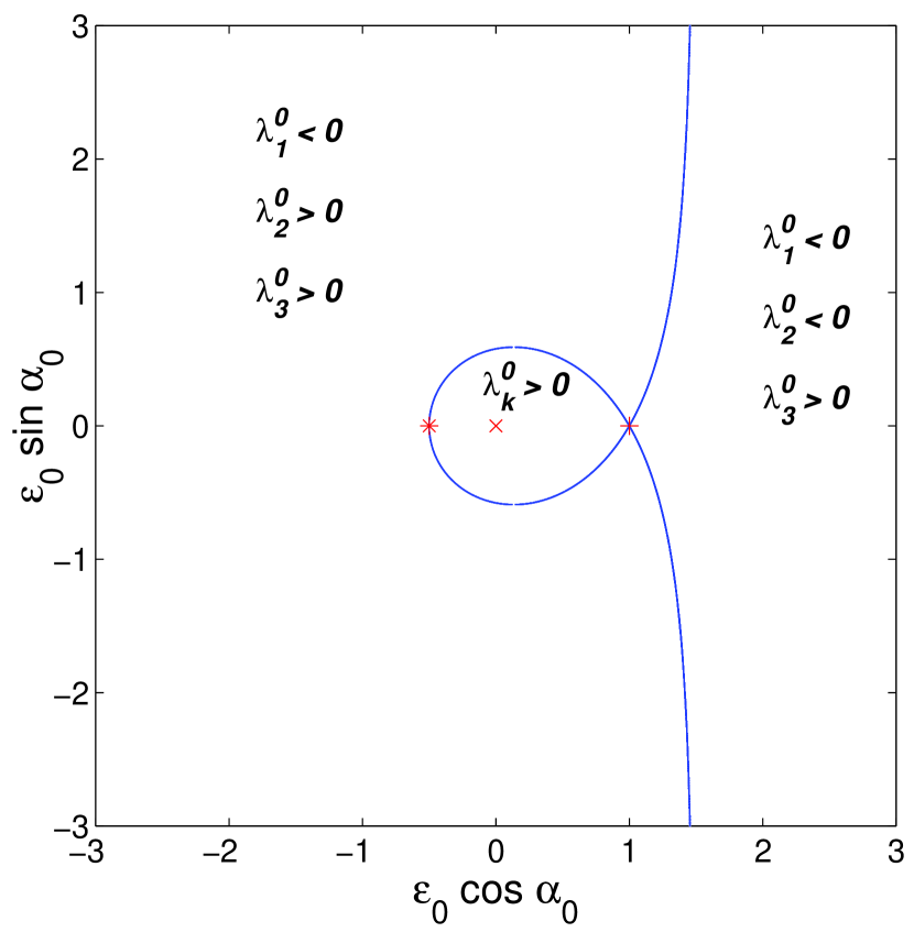
Figure 2: (c) The same as (a) except that the DTA is used. The innermost contour is $a_{c}=1.6$. (d) The same as (a) except that the CZA is used. The innermost contour is $a_{c}=1.7$. (e) The same as (a) except that the LTA is used. The innermost contour is $a_{c}=1.6$. (f) The signs of $\lambda^{0}_{i}$ in each region of the parameter space of initial conditions, with $\delta_{0}=+1$. The inner region corresponds to the values of $\lambda^{0}_{i}$ that can be spanned by a homogeneous ellipsoid with any axes ratios. Spherical, planar, and cylindrically symmetric perturbations are marked with a cross, a plus sign, and a star respectively. The upper part of these graphs, which correspond to $0\leq\alpha_{0}\leq\pi$, have $\lambda^{0}_{3}>\lambda^{0}_{2}>\lambda^{0}_{1}$. The lower one covers the same values of $\lambda^{0}_{i}$, through a permutation of the indices.

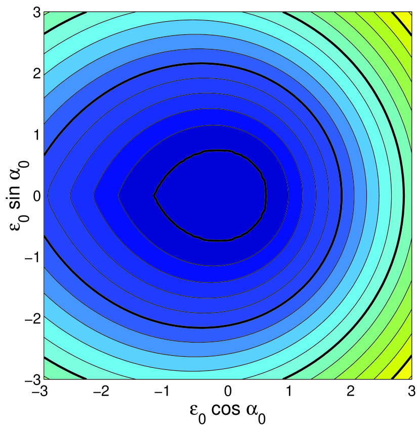
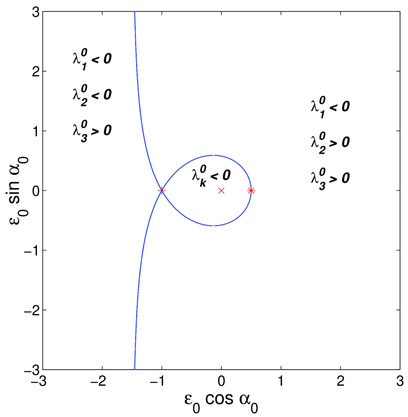
Figure 4: (a) The collapse time as a function of the initial conditions for underdense perturbations with $\delta_{0}=-1$. The contours of constant collapse time, expressed by $a_{c}^{-1}$, are displayed for the ZA. The light (heavy) contours are spaced by 0.1 (0.5) in $a_{c}^{-1}$, with the innermost contour being $a_{c}^{-1}=0$. Initial perturbations in the central region do not collapse. (b) The same as (a) except that the DTA is used. (c) The same as (a) except that the LTA is used. (d) The signs of $\lambda^{0}_{i}$ corresponding to each region of the parameter space of initial conditions, with $\delta_{0}=-1$. Spherical, planar, and cylindrically symmetric underdense perturbations are marked with a cross, a plus sign, and a star respectively. The upper part of these graphs, which correspond to $0\leq\alpha_{0}\leq\pi$, have $\lambda^{0}_{3}>\lambda^{0}_{2}>\lambda^{0}_{1}$. The lower one covers the same values of $\lambda^{0}_{i}$, through a permutation of the indices.

In Figures 2 and 4, we plot the collapse time $a_{c}$ as a function of $\varepsilon_{0}$ and $\alpha_{0}$ for overdense and underdense perturbations, respectively. Since the MZA and CZA do not apply for some underdense regions, we have not displayed the results of these approximations in figure 4. We also show the signs of $\lambda^{0}_{i}$ corresponding to the initial conditions in these two figures.

The parameter space of initial conditions that can be spanned by an ellipsoid with any axes ratios is equivalent to having the three $\lambda^{0}_{i}$ positive. The region corresponding to the homogeneous ellipsoid is limited to relatively small shear, and all the local approximations, except for the ZA, agree significantly well in this region. The ZA overestimates the collapse time for spherical configurations. We see that they still quite similar for overdense perturbations in general. The MZA substantially deviates from the others for high shear. In all the cases the shear accelerates the collapse, which is a well-known nonlinear effect. Thus the first regions to collapse are not necessarily those with higher density. We can also see that oblate initial configurations (for which $\cos\alpha_{0}>0$) collapse first. Thus planar collapse is favored by these approximations.

For negative perturbations the difference among the approximations is enhanced. The LTA systematically gives slightly larger collapse times than the DTA. The collapse time given by the ZA is the shortest among the three. It is important to notice that in the local approximations underdense regions may also collapse, due to the effects of the shear.

The relevance of the shear in the nonlinear phase of gravitational clustering is in agreement with $N$-body simulations (Katz, Quinn, & Gelb 1993), yet it is sometimes ignored in structure formation studies. Any model based on the spherical collapse would miss this effect.

An interesting aspect of the local approximations is that the collapse time has the same asymptotic behavior

$$a_{c}\left(\delta_{0},\varepsilon_{0},\alpha_{0}\right)\simeq\frac{C}{\varepsilon_{0}}$$ (41)

for high initial shear ($\varepsilon_{0}\gg\delta_{0}$) in all the approximations, where $C$ is a (slowly varying) function of $\alpha_{0}$ only (see Appendix A). That is, the collapse time for large shear does not depend on $\delta_{0}$ and is inversely proportional to the initial shear $\varepsilon_{0}$.

3.3 The Cosmological Mass Function

The mass function $n\left(M\right)$ is defined such that $n\left(M\right)dM$ gives the number density of collapsed dark matter clumps with masses between $M$ and $M+dM$. These clumps are associated with proto-galactic haloes, and with galaxy groups and clusters. Comparing theoretical mass functions with observations provides important constraints on the cosmological parameters (Bahcall & Cen 1993; Girardi et al. 1998; Rahman & Shandarin 2000) and the spectrum of primordial perturbations (Lucchin & Matarrese 1988; Ribeiro, Wuensche, & Letelier 2000). The approach of Press & Schechter (1974) to calculate the mass function, hereafter PS, has been extended to nonspherical collapse and applied to some local approximations (Monaco 1995 for the ZA, and Audit et al. 1997 for the DTA). Here, we extend such analysis to the LTA and compare them.

Let $F\left(M;a_{0}\right)$ be the fraction of collapsed objects at $a_{0}$ with mass higher than $M$; then the mass function is given by

$$n\left(M\right)=-\frac{\bar{\rho}}{M}\frac{dF}{dM}.$$ (42)

The fraction $F$ may be calculated as an integral over all the possible initial conditions weighted by their probabilities:

$$F=\frac{1}{F_{0}}\int_{0}^{\pi}\int_{0}^{\infty}\int_{-\infty}^{+\infty}s\left(a_{0};\delta_{0},\varepsilon_{0},\alpha_{0}\right)P_{M}\left(\delta_{0},\varepsilon_{0},\alpha_{0}\right)d\delta_{0}d\varepsilon_{0}d\alpha_{0}.$$ (43)

The function $s$ is equal to one if an element with parameters $\delta_{0},\varepsilon_{0},\alpha_{0}$ has already collapsed at $a_{0}$, and is zero otherwise; $F_{0}$ is a normalization factor. The collapse time $a_{c}$ of a fluid element with initial perturbations parametrized by $\delta_{0},\varepsilon_{0},\alpha_{0}$ can be computed in the local approximations. As mentioned in subsection 2.6, the collapse is characterized by the divergence of the density, which is equivalent to the first axis collapse. Beyond this point the Lagrangian formalism breaks down. Some authors (Audit et al. 1997; Lee & Shandarin 1998; Sheth, Mo & Tormen 1999) have suggested other alternatives for the definition of collapse in the calculation of the mass function. Here we will prefer to keep the simplest assumption of first axis collapse, since it does not introduce any free parameter.

What we need now is the probability distribution function $P_{M}\left(\delta_{0},\varepsilon_{0},\alpha_{0}\right)$ for the initial conditions. Assuming Gaussian initial fluctuations, Doroshkevich (1970) derived the joint probability for the three eigenvalues of the deformation tensor $\lambda_{1}^{0},\lambda_{2}^{0}$ and $\lambda_{3}^{0}$. Using this result, $P_{M}\left(\delta_{0},\varepsilon_{0},\alpha_{0}\right)$ is given by the product of three independent probabilities for each parameter $\delta_{0}$, $\varepsilon_{0}$ and $\alpha_{0}$:

$$P_{\nu}\left(\delta_{0}\right) = \frac{1}{\sqrt{2\pi\Delta^{2}}}\exp\left[-\frac{1}{2}\left(\frac{\delta_{0}}{\Delta}\right)^{2}\right],$$ (44)

$$P_{\chi}\left(\varepsilon_{0}\right) = \frac{50}{3}\sqrt{\frac{5}{2\pi\Delta^{2}}}\left(\frac{\varepsilon_{0}}{\Delta}\right)^{4}\exp\left[-\frac{5}{2}\left(\frac{\varepsilon_{0}}{\Delta}\right)^{2}\right],$$ (45)

$$P_{\alpha}\left(\alpha_{0}\right) = \sin\left(\frac{\alpha_{0}}{3}\right)\left[\frac{3}{2}-2\sin^{2}\left(\frac{\alpha_{0}}{3}\right)\right].$$ (46)

The variance $\Delta$ is related to the mass $M$ and the power spectrum of the primordial density field $\sigma_{k}$ through

$$\Delta^{2}\left(R\right)=\int_{0}^{\infty}\frac{dk}{2\pi^{2}}W_{k}^{2}\left(R\right)k^{2}\sigma_{k}^{2},$$ (47)

where $M=(4\pi/3)f_{W}R^{3}\bar{\rho}$ and $W_{k}\left(R\right)$ is the Fourier transform of a filter with width $R$ in physical space. The factor $f_{W}$ depends on the shape of the filter function, for a top-hat filter we have $f_{W}=1$, whereas for a sharp$-k$ filter $f_{W}=9\pi/2$. The mass function can now be written in the form

$$n\left(M\right)=-\frac{\bar{\rho}}{M}\frac{d\Delta}{dM}\Phi\left(\Delta\right),$$ (48)

where $\Phi\left(\Delta\right)=dF(\Delta)/d\Delta$. The function $\Phi\left(\Delta\right)$ contains all the influence of the dynamics and depends neither on the particular form of the power spectrum nor of the filter $W$; it is referred to as the universal mass function (Audit et al. 1997).

We calculate the universal mass function for the ZA, LTA and DTA but not for the MZA and CZA since they do not apply for negative density perturbations. In appendix B we show the detailed calculation.

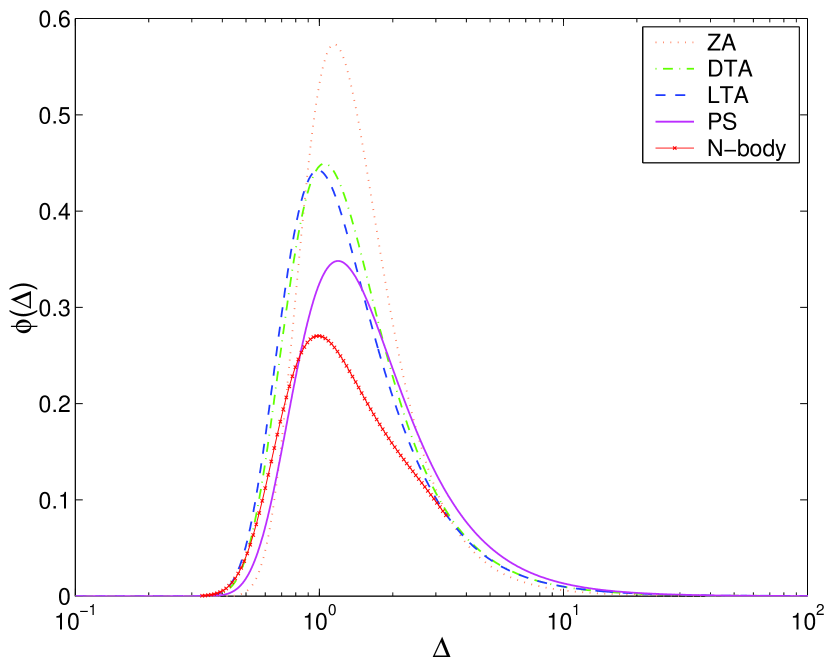
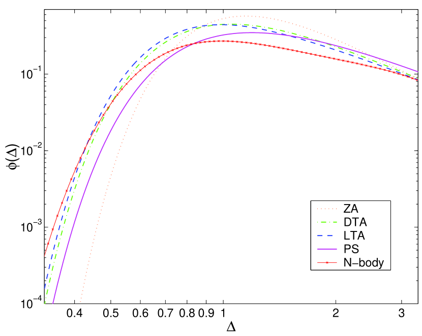
Figure 5: (a) The universal mass function calculated for the ZA (dotted curve), the DTA (dash-dotted curve) and the LTA (dashed curve). For comparison, we display in this figure the fit to $N$-body simulations (line+cross) obtained by Jenkins et al. (2000), together with the standard PS mass function (solid curve). (b) The same as (a) but now a logarithmic scale is used in the $y$ axis. Here the $x$ axis scale is limited to the range $0.332\leq\Delta\leq 3.32$ covered by the $N$-body simulations.

In Figure 5, we show the mass functions for those approximations. For comparison, we also display in this figure the fit to $N$-body simulations obtained by Jenkins et al. (2000), together with the standard PS mass function.

We see that the results of the DTA and LTA are very similar. Furthermore, in the high-mass tail ($\Delta\lesssim 0.5$), they reproduce well the results of the $N$-body simulations. However, we can see that these approximations overestimate the concentration of masses near $\Delta=1$. The right-end tail of the distribution decays more rapidly compared to the $N$-body simulations. This tendency is still enhanced in the ZA. However, in these approximations, the position of the maximum of the distribution is close to that of the $N$-body simulations, giving a better estimate than that of the PS; in particular, the LTA and DTA give nearly the same value as the $N$-body results.

As for the normalization factor $F_{0}$, there exists an extensive discussion on its origin (see, for example, Peacock & Heavens 1990; Bond et al. 1991; Jedamzik 1995; Yano, Nagashima, & Gouda 1996). The normalization factors for the local approximations are close to one ($1/0.92$ for the DTA, and $1/0.89$ for the LTA) whereas in the original PS derivation the normalization factor needed is $F_{0}=1/0.5$. This is due to the fact that, in the spherical collapse model, only overdense regions collapse.

The fact that around $\Delta=1$ the number of objects is overestimated in the local approximations implies, due to the normalization of the mass function, that they should provide a lower estimate than the $N$-body simulations for large enough $\Delta$. There, the contribution from the low-mass objects is dominant; in any realistic process, they may also arise from the fragmentation of larger clusters. The criterion for the formation of a clump from the direct collapse of an initially perturbed region does not account for these complex processes of fragmentation. Therefore, the discrepancy of the mass function for high $\Delta$ might be attributed to the use of expression (43) rather than to the definition (42).

4 DISCUSSION

We have investigated local Lagrangian approximations to the nonlinear dynamics of pressureless dark matter. We have selected the modified Zel’dovich approximation (MZA), the deformation tensor approximation (DTA), the complete Zel’dovich approximation (CZA), and the local tidal approximation (LTA), in addition to the original Zel’dovich approximation (ZA). These four approximations were designed to improve the ZA, and are in fact exact for planar, spherical and cylindrical symmetries, whereas the ZA is only exact for the planar case. They are semi-analytic and easy to be implemented in any application where local quantities are involved, such as the calculation of the mass function in the PS approach.

All the local approximations discussed here, except for the ZA, provide quite a similar evolution for an ellipsoid, reproducing the results of the homogeneous ellipsoid model. Thus, for this kind of positive density perturbations, these methods work fairly well. However, the MZA turns out to deviate substantially for large values of the shear as was shown in section (3.2), reflecting the fact that it does not give the correct second order solution. Furthermore, the MZA cannot deal with initially underdense regions that will eventually collapse. Therefore, its applicability is rather limited when compared to the other approximations.

We note that the second order expansions of the CZA, LTA and DTA coincide with the second order Lagrangian perturbation theory, whereas those of the MZA and ZA do not. It is interesting to recall that the LTA and DTA have very different origins from the CZA, but still they give the correct second order result.

The CZA, LTA and DTA give quite analogous results for generic initial conditions. However, at least in its original form, the CZA cannot be used for negative values of $\lambda_{i}$. One possible solution to this problem might be achieved through an expansion such as

$$r_{i}=\frac{1+\sum_{l,m,n=0}^{N}E_{l,m,n}^{p}(\lambda_{j}+\lambda_{k})^{l}(\lambda_{j}-\lambda_{k})^{2n}\lambda_{i}^{m}}{1+\sum_{l,m,n=0}^{M}D_{l,m,n}^{p}(\lambda_{j}+\lambda_{k})^{l}(\lambda_{j}-\lambda_{k})^{2n}\lambda_{i}^{m}}.$$ (49)

The coefficients $E$ and $D$ should be appropriately chosen to adjust the asymptotic behavior; in particular, we could use the numerical solution for underdense cylindrical and spherical perturbations to fit some of these coefficients, as done for the overdense case in the CZA. Besides, to agree with the perturbative solution (18) we should have

$$E_{l,m,n}^{1}-D_{l,m,n}^{1}=C_{l,m,n}^{1}.$$ (50)

For higher orders, the determination of these coefficients is rather complicated. Further investigations on this possibility should be pursued.

Concerning the mass function, it is found that the LTA and DTA give an accurate result for large masses as compared to the $N$-body simulations. The position of the peak is also in good agreement, whereas its amplitude is overestimated by a factor 2 compared to the $N$-body results. Since the mass function is normalized to unity, this means that the local approximations, together with the PS formalism, underestimates the density of low-mass clusters. However, this might be a consequence of the criterion for the formation of a collapsed object based only on the collapse time.

It is interesting to notice that the collapse time, as a function of $\alpha_{0}$ and $\varepsilon_{0},$ has an approximate scaling property (see eq. A1), which is very precise for $\varepsilon_{0}/\delta_{0}\gg 1$. We conclude that this may be a general feature of gravitational collapse in local approximations, whose validity is worth checking in a more general setting.

While there is still not a clear theoretical understanding or support to the local approximations, they proved to be very accurate in the situations investigated here. They reproduce some well known features of nonspherical collapse, such as the possibility of collapse of some initially underdense regions, and the fact that the shear accelerates the collapse (see Sahni & Coles 1995). The main limitation of these approximations is that they only provide information about the internal state of a given mass element, but do not determine its position. Even so, their simplicity is highly expedient for practical applications, such as the calculation of nonlinear corrections to the microwave background anisotropies, and the Gunn-Peterson effect. In particular, they are suitable for obtaining statistical properties of the present fields as a function of the primordial ones, as in the case of the mass function. Further studies on the validity of these approximations, based on a comparison to $N$-body simulations, are required. Such a comparison would allow to fully test the approximations described in this paper and more generically, the locality hypothesis. If they still provide accurate results in this case, the local approximations could represent good alternatives to the computer simulations, taking much less computational time, allowing thereby a larger scanning of initial conditions. They could give complementary information to the $N$-body simulations and would provide a better physical understanding of the nonlinear dynamics of self gravitating systems.

Most of the results of this paper may be extended to more general backgrounds. The influence of any smooth component only alters the behavior of $a(t)$, and of the growing mode growth factor $D\left(t\right)$, that will not be equal any more. It would be interesting to study the relativistic analogue of the LTA. Another interesting extension would be to include vorticity in the local approximations as was done for the ZA in (Buchert 1992; Barrow & Saich 1993). We could use them to test the effects of a possible primeval vorticity on large scales (Li Xin-Li 1998).

Appendix A FITTING FORMULAE FOR THE COLLAPSE TIME

In order to avoid repeated numerical integrations of differential equations in the LTA and DTA, we have parametrized the collapse time as a function of initial conditions. For both of these local approximations, the following scaling property is approximately satisfied:

$$a_{c}^{\pm}\left(x,\alpha_{0}\right)\simeq H^{\pm}\left(f\right),\;\mathrm{with\;}f=xg^{\pm}\left(\alpha_{0}\right),$$ (A1)

where $H^{\pm}$ and $g^{\pm}$ are functions to be fitted for each approximation, and $x=\varepsilon_{0}/\left|\delta_{0}\right|$. This relation becomes more accurate for increasing $x$. In any case the error of the fit is less than a few percent.

For $g\left(\alpha\right)$ we found that a kind of truncated Fourier series can be used to a very good approximation:

$$g\left(\alpha\right) = c_{1}\cos\left(\frac{\alpha}{2}\right)+c_{2}\cos\alpha+c_{3}\cos\left(\frac{3\alpha}{2}\right)+c_{4}\cos\left(2\alpha\right)+$$ (A2)

$$c_{5}\cos\left(\frac{5\alpha}{2}\right)+\left(1-c_{1}-c_{2}-c_{3}-c_{4}-c_{5}\right)\cos\left(3\alpha\right).$$

The values of the parameters for each case are shown in Table 2.

Table 2: Parameters of $g(\alpha)$ fitted for the LTA and DTA

$g$	$c_{1}$	$c_{2}$	$c_{3}$	$c_{4}$	$c_{5}$
$g_{LTA}^{+}$	1.546	-1.015	0.786	-0.462	0.182
$g_{LTA}^{-}$	1.461	-0.767	0.473	-0.231	0.079
$g_{DTA}^{+}$	1.505	-0.842	0.508	-0.228	0.066
$g_{DTA}^{-}$	1.497	-0.836	0.513	-0.234	0.068

For the dependence of $a_{c}$ on $x$ for fixed $\alpha_{0}$, we fitted the function $f=H^{-1}$ rather than $H$ itself, because this is the quantity we will need to compute the mass function. Taking into account the boundary value and asymptotic behavior, we parametrize $f$ by

$$f^{+}=\frac{d_{1}z\left(1+d_{2}z+d_{4}z^{2}\right)}{\left(1+d_{3}z+d_{5}z^{2}\right)a_{c}},\;\mathrm{with\;}z=d_{0}-a_{c},$$ (A3)

for overdense regions ($\delta_{0}>0$), and

$$f^{-}=d_{0}+\frac{d_{1}a_{c}^{-1/2}\left(1+d_{2}a_{c}^{-1}+d_{4}a_{c}^{-5/2}\right)}{1+d_{3}a_{c}^{-1}+d_{5}a_{c}^{-2}},$$ (A4)

for underdense regions ($\delta_{0}<0$). The parameters for the LTA and DTA are given in Table 3.

Table 3: Parameters of $f$ fitted for the LTA and DTA

$f$	$d_{0}$	$d_{1}$	$d_{2}$	$d_{3}$	$d_{4}$	$d_{5}$
$f_{LTA}^{+}$	$1.686$	$8.469$	$19.88$	$78.49$	$17.03$	$163.2$
$f_{DTA}^{+}$	$1.686$	$14.14$	$13.34$	$87.68$	$8.676$	$163.8$
$f_{LTA}^{-}$	$0.591$	$1.064$	$0.678$	$-1.335$	$16.054$	$8.613$
$f_{DTA}^{-}$	$0.495$	$0.942$	$0.322$	$-2.083$	$25.718$	$12.961$

Notice that for high shear ($x\gg 1$) we have $a_{c}\ll 1$ such that:

$$a_{c}^{+}\underset{x\rightarrow\infty}{\longrightarrow}\frac{d_{1}d_{0}\left(1+d_{2}d_{0}+d_{4}d_{0}^{2}\right)}{\left(1+d_{3}d_{0}+d_{5}d_{0}^{2}\right)}\frac{1}{xg^{+}\left(\alpha_{0}\right)}.$$ (A5)

and

$$a_{c}^{-}\underset{x\rightarrow\infty}{\longrightarrow}\frac{d_{1}d_{4}}{d_{5}}\frac{1}{xg^{-}\left(\alpha_{0}\right)},$$ (A6)

In the Zel’dovich approximation we have an analytical expression for $a_{c}$. As the collapse occurs when the greatest $\lambda_{i}$ reaches the value $1$, using the parametrization (36) we get:

$$a_{c}^{ZA}=\frac{3}{\delta_{0}+2\varepsilon_{0}\cos\left(\alpha_{0}/3\right)}.$$ (A7)

In this case we can clearly see the features of $a_{c}$:

$$a_{c}^{ZA}\left(\delta_{0},\varepsilon_{0},\alpha_{0}\right) = \frac{1}{\left|\delta_{0}\right|}\frac{3}{\pm 1+2\left(\varepsilon_{0}/\left|\delta_{0}\right|\right)\cos\left(\alpha_{0}/3\right)}$$ (A8)

$$= \frac{1}{\left|\delta_{0}\right|}a_{c}^{ZA}\left(\pm 1,\varepsilon_{0}/\left|\delta_{0}\right|,\alpha_{0}\right).$$

Note that the property (A1) is satisfied exactly for the ZA.

Appendix B CALCULATION OF THE MASS FUNCTION

With the integral (43) we may write the universal mass function $\Phi\left(\Delta\right)=dF/d\Delta$ in the form

$$\Phi\left(\Delta\right)=\frac{1}{F_{0}}\frac{d}{d\Delta}\int_{0}^{\pi}\int_{0}^{\infty}\int_{-\infty}^{+\infty}s\left(\nu\Delta,\chi\Delta,\alpha_{0}\right)P\left(\nu,\chi,\alpha_{0}\right)d\nu d\chi d\alpha_{0},$$ (B1)

where $\nu=\delta_{0}/\Delta$ and $\chi=\varepsilon_{0}/\Delta$. With these new variables the dependence on $\Delta$ will be present only in the function $s$, which may be written as

$$s=\Theta\left(1-a_{c}\left(\delta_{0},\varepsilon_{0},\alpha_{0}\right)\right).$$ (B2)

Note that in the case of the Press & Schechter original approach this function is given by: $s=\Theta\left(\delta_{0}-\delta_{c}\right),$ where $\delta_{c}=1.686$ is the value at which a spherical perturbation collapses at $a=1$.

To calculate $ds/d\Delta$ one uses the relation (40), obtaining:

$$\frac{ds}{d\Delta}=\delta_{D}\left(1-a_{c}\left(\nu\Delta,\chi\Delta,\alpha_{0}\right)\right)\frac{a_{c}^{\pm}\left(\chi/\nu,\alpha_{0}\right)}{\left|\nu\right|\Delta^{2}},$$ (B3)

where $\delta_{D}$ is the Dirac delta function. Therefore we may eliminate one of the integrals in expression (B1), with the mass function being calculated over the surface $a_{c}\left(\nu\Delta,\chi\Delta,\alpha_{0}\right)=\left|\nu\Delta\right|^{-1}a_{c}^{\pm}\left(\chi/\nu,\alpha_{0}\right)$ $=1$. For this sake we need to write one of the three variables in terms of the others on this surface.

Let us assume the we have $\chi$ as a functions of $\nu\Delta$ and $\alpha$: $\chi=\chi_{a}\left(\nu\Delta,\alpha\right)$, where the subscript $a$ indicates that $\chi$ is calculated over the surface $a_{c}=1$. The integral in $\chi$ in equation (B1) is thus eliminated using the relation

$$\delta_{D}\left(1-a_{c}\left(\nu\Delta,\chi\Delta,\alpha_{0}\right)\right)=\delta_{D}\left(\chi-\chi_{a}\right)\left|\frac{\partial a_{c}}{\partial\chi}\right|^{-1}.$$ (B4)

The mass function (B1) is now given by:

$$\Phi\left(\Delta\right)=\frac{1}{F_{0}}\int_{0}^{\pi}\int_{-\infty}^{+\infty}\frac{1}{\Delta}\left|\frac{\partial a_{c}}{\partial\chi}\right|^{-1}P_{\nu}\left(\nu\right)P_{\chi}\left(\chi_{a}\right)P_{\alpha}\left(\alpha_{0}\right)d\nu d\alpha_{0},$$ (B5)

where $\partial a_{c}/\partial\chi$ is evaluated in $\chi_{a}\left(\nu\Delta,\alpha\right).$ We can simplify this expression further if the collapse time $a_{c}\left(x,\alpha\right)$ is only a function of the product $xg\left(\alpha\right),$ which we have seen is an excellent approximation for the local approximations studied here (see appendix A). Using the property (A1) we have

$$\chi_{a}=\frac{\nu}{g\left(\alpha_{0}\right)}H^{-1}\left(\left|\nu\Delta\right|\right),$$ (B6)

and

$$\left|\frac{\partial a_{c}}{\partial\chi}\right|=\left|\frac{1}{\nu\Delta}\frac{\partial H}{\partial f}\frac{g\left(\alpha_{0}\right)}{\nu}\right|,$$ (B7)

where the superscript $+$ is implied for positive $\nu$, and the $-$ for negative $\nu$. Replacing these results in expression (B5) we get finally:

$$\Phi\left(\Delta\right)=\frac{1}{F_{0}}\int_{-\infty}^{+\infty}\int_{0}^{\pi}\nu^{2}\left|\left(\frac{\partial H}{\partial f}\right)^{-1}\frac{1}{g\left(\alpha_{0}\right)}\right|P_{\nu}\left(\nu\right)P_{\chi}\left(\chi_{a}\right)P_{\alpha}\left(\alpha_{0}\right)d\alpha_{0}d\nu,$$ (B8)

where $\chi_{a}=\left|\nu\right|f_{a}/g\left(\alpha_{0}\right)$, with $f_{a}\left(\nu\Delta\right)=H^{-1}\left(\left|\nu\Delta\right|\right)$ and $\partial H/\partial f$, is calculated in $f_{a}$. This is why we have chosen to fit the function $H^{-1}$, instead of its inverse.

As $P\left(\nu\right)$ and $\partial H/\partial f$ are independent of $\alpha_{0},$ we integrate first in this variable:

$$I_{1}\left(\nu,\Delta\right):=\int_{0}^{\pi}\frac{1}{g^{5}\left(\alpha_{0}\right)}\exp\left[-\frac{5}{2}\left(\frac{\nu f}{g\left(\alpha_{0}\right)}\right)^{2}\right]P_{\alpha}\left(\alpha_{0}\right)d\alpha_{0}.$$ (B9)

The universal mass function will now be given by

$$\Phi\left(\Delta\right)=\frac{1}{F_{0}}N\int_{-\infty}^{+\infty}I_{1}\left(\nu,\Delta\right)\nu^{6}f_{a}^{4}\left|\left(\left.\frac{\partial H}{\partial f}\right|_{f_{a}}\right)^{-1}\right|\exp\left(-\frac{\nu^{2}}{2}\right)d\nu.$$ (B10)

where $N=50\sqrt{5}/6\pi$ is the product of the normalizations for $P_{\nu}$ and $P_{\chi}$ (equations (44) and (45)). Note that the above integral is limited for positive values of $\nu$, as $H^{-1}\left(\left|\nu\Delta\right|\right)=0$ for $\nu\Delta>f_{0}$ ($f_{0}=1.686$ for the DTA and LTA, and $f_{0}=3$, for the ZA). Although our fitting formulas (sec. A) become less accurate for $\nu\rightarrow-\infty$ and $\nu\rightarrow f_{0}/\Delta,$ the mass function is not affected, since the integrand in (B10) goes to zero in these regions. Here it is clear that the underdense regions do contribute to the mass function, as pointed out by Audit et al. (1997).

As an example, let us consider the Zel’dovich approximation. In this case we have

$$H_{\pm}\left(f\right)=\frac{3}{\pm 1+2f},\;\mathrm{and\;}g\left(\alpha\right)=\cos\left(\frac{\alpha}{3}\right).$$ (B11)

Using the following transformation of variables

$$x=\sin\left(\frac{\alpha}{3}\right)\rightarrow P_{\alpha}d\alpha=x\left[\frac{3}{2}-2x^{2}\right]3\frac{dx}{\sqrt{1-x^{2}}},$$ (B12)

we find an analytical expression for the integral (B9):

$$I_{1}:=\frac{1}{\left(\nu f\right)^{2}}\exp\left[-\frac{5}{2}\left(\nu f\right)^{2}\right]\left[\frac{3}{25}\frac{1}{\left(\nu f\right)^{2}}\left(\exp\left[-\frac{15}{2}\left(\nu f\right)^{2}\right]-1\right)+\frac{9}{10}\right],$$ (B13)

where $f^{\pm}=\left(3/\left(\left|\nu\right|\Delta\right)\mp 1\right)/2$. The mass function will be given by:

$$\Phi\left(\Delta\right) = \frac{1}{F_{0}}\frac{15\sqrt{5}}{8\pi}\int_{-\infty}^{+\infty}\frac{1}{\Delta^{4}}\exp\left(-\frac{\nu^{2}}{2}\right)\exp\left[-\frac{5}{8}\frac{\left(3-\nu\Delta\right)^{2}}{\Delta^{2}}\right]\times$$ (B14)

$$\left[\frac{12}{5}\Delta^{2}\left(\exp\left[-\frac{15}{8}\frac{\left(3-\nu\Delta\right)^{2}}{\Delta^{2}}\right]-1\right)+\frac{9}{2}\left(3-\nu\Delta\right)^{2}\right]d\nu.$$

Figure 1: Evolution of the three axes $R_{i}$ of an ellipsoid according to the homogeneously collapsing ellipsoid model (HCE, solid curve), and the five approximations considered in the text: Zel’dovich (ZA, dotted curve), Modified Zel’dovich (MZA, short dot), Deformation Tensor (DTA, dash-dot), Complete Zel’dovich (CZA, short dash) and Local Tidal (LTA, long dash). The initial axes ratios are $1:1.25:1.5$ and the density contrast linearly extrapolated to $a=1$ is $\delta_{0}=1$. The ZA overestimates the collapse time, whereas all other approximations are close to the HCE.

Figure 2: (a) The collapse time as a function of the initial conditions for overdense perturbations with $\delta_{0}=+1$. The contours of constant collapse time, expressed by the scale factor $a_{c}$, are displayed for the ZA. The light (heavy) contours are spaced by 0.1 (0.5) in $a_{c}$, with the outermost contour being $a_{c}=0.4$ and the central velue $a_{c}=3$. (b) The same as (a) except that the MZA is used. The innermost contour is $a_{c}=1.6$.

References

- (1) Audit, E., & Alimi, J.-M. 1996, A&A, 315, 11
- (2) Audit, E., Teyssier, R, & Alimi, J.-M. 1997, A&A, 325, 439
- (3) Bahcall, N. A, & Cen, R. 1993, ApJ, 407, L49
- (4) Barnes, A. & Rowlingson, R. 1989, Class. Quantum Grav., 6, 949
- (5) Barrow, J. D. & Saich, P. 1993, Class. Quantum. Grav. 10, 79
- (6) Bertschinger, E., & Jain, B. 1994, ApJ, 431, 486
- (7) Bertschinger, E., & Hamilton, A. J. S. 1994, ApJ, 435, 1
- (8) Bertschinger, E. 1996, in XV Les Houches Summer School, Cosmology and Large Scale Structure, ed. R. Schaeffer, J. Silk, M. Spiro and V. Zinn-Justin (Amsterdam: Elsevier)
- (9) Bertschinger, E. 1998, ARA&A, 36, 599
- (10) Betancort-Rijo, J., & López-Corredoira, M. 2000, ApJ, 534, L117
- (11) Bond, J. R., Cole, S., Efstathiou, & G., Kaiser, N 1991, ApJ, 379, 440
- (12) Buchert, T 1992, MNRAS, 254, 729
- (13) Buchert, T 1994, MNRAS, 267, 811
- (14) Carlson, B. C. 1977, SIAM J. Math. Anal., 8, 231
- (15) De Bernardis, P., et al. 2000, Nature, 404, 945
- (16) Doroshkevich, A. G. 1970, Astrofizika, 6, 581 (English translation: Astrophysics, 6, 320)
- (17) Durrer, R. & Novosyadlyj, B. 2000, MNRAS, submitted (astro-ph/0009057)
- (18) Eisenstein, D., J., Loeb 1995, ApJ, 439, 520
- (19) Ellis G. F. R. 1973, in Cargèse Lectures on Physics Vol. 6, Relativistic Cosmology, ed. E. Schatzman (New York: Gordon and Breach), 1
- (20) Ellis, G. F. R., & Dunsby, P. K. S. 1997, ApJ, 479, 97
- (21) Girardi, M., Borgani, S., Giuricin, R., Mardirossian, F., & Mezzetti, M. 1998, ApJ, 506, 45
- (22) Hanany, S., et al 2000, ApJL, in press (astro-ph/0005123)
- (23) Hui, L., & Bertschinger, E., 1996, ApJ, 471, 1
- (24) Icke, V. 1973, A&A, 27, 1
- (25) Jedamzik, K 1995, ApJ, 448
- (26) Jenkins, A., Frenk, C. S., White, S. D. M., & Colberg, J. M. 2000, MNRAS, in press (astro-ph/0005260)
- (27) Juszkiewicz, R., Bouchet, F. R., & Colombi, S. 1993, ApJ, 412, L9
- (28) Katz, N., Quinn, T., & Gelb, J. M. 1993, MNRAS, 265, 689
- (29) Kofman, L., & Pogosyan, D. 1995, ApJ, 442, 30
- (30) Li, L.-X. 1998, Gen. Rel. Grav. 30, 497
- (31) Lacey, C., & Cole, S. 1993, MNRAS, 262, 627
- (32) Lachièze-Rey, M. 1993, ApJ, 408, 403
- (33) Lee, J., & Shandarin, S. 1998, ApJ, 500, 14
- (34) Lucchin, F., & Matarrese, S. 1988, ApJ, 330, 535
- (35) Matarrese, S., Pantano, O., Saez, D. 1993, 47, 4, 1311
- (36) Monaco, P. 1995, ApJ, 447, 23
- (37) Moutarde, F., Alimi, J.-M., Bouchet, F. R., Pellat, R., Ramani, A. 1991, ApJ, 382, 424
- (38) Press, W. H., Teukolsky, S. A., Vetterling, W. T., Flannery, B. P. 1992, Numerical Recipes in Fortran: The Art of Scientific Computing (2nd. ed.; Cambridge: Cambridge University Press)
- (39) Peacock, J. A., & Heavens, A. F. 1990, Mon. Not. R. Astron. Soc., 243, 133
- (40) Press, W. H., & Schechter, P. 1974, ApJ, 187, 425
- (41) Perlmuter, S., et al. 1998, Nature, 391, 51
- (42) Rahman, N., & Shandarin, S. 2000, ApJL, submitted (astro-ph/0010228)
- (43) Reisenegger, A., & Miralda-Escudé, J. 1995, ApJ, 449, 476
- (44) Ribeiro, A. L. B., Wuensche, C. A., & Letelier, P. S. 2000, ApJ, 539, 4.
- (45) Riess, A. G., et al. 1998, AJ, 116, 100
- (46) Sheth, R. K., Mo, H. J., & Tormen, G. 1999, preprint (astro-ph/9907024)
- (47) Sahni, V., & Coles, P. 1995, Phys. Rep. 1995, 262, 1
- (48) Turner, M. 2000, Phys. Rep., 333, 619
- (49) White, S. D. M., & Silk, J. 1979, ApJ, 231, 1
- (50) Yano, T. , Nagashima, M., & Gouda, N. 1996, ApJ, 466, 1
- (51) Zehavi, I. & Dekel, A. 1999, Nature, 401, 252
- (52) Zel’dovich, Ya. B. 1970, A&A, 5, 84