Derivation of preliminary IBIS response matrices with the INTEGRAL Simulator

Abstract

We have used the IBIS Simulator to produce preliminary response matrices for the ISGRI and PICsIT detectors in order to help understanding their scientific performances before the calibration results are available. The derived matrices, in a format compatible with the XSPEC spectral analysis package, have been tested by fitting simple models and then used to analyze simulations of astrophysical sources with more complex spectra.

1 The Simulator

The IBIS Simulator (developed in collaboration by IFC/CNR Milan, Southampton University and ISDC) can perform the following steps. It first generates a model of the gamma-ray sky with the possibility of defining position, intensity and spectral properties of the celestial sources. Then different observation strategies (pointing directions, observation length, dithering patterns, etc.) can be defined. After these preliminary steps the interaction of all the source photons with the active and passive materials of the instruments are simulated. An estimate of the background is also added, based on the results of the INTEGRAL Mass Model (Lei et al. 1999), which is a detailed Monte Carlo simulation that takes into account the interaction of the particle and photon flux with the whole INTEGRAL spacecraft. The Simulator finally produces a data set in a format fully compatible with the ISDC analysis system. For the analysis of the output data we have developed some prototype programs, which perform image deconvolution and spectral extraction.

2 Building the response matrices

To build the response matrices of ISGRI and PICsIT (Ubertini et al. 1999), two sets of simulations of on-axis monochromatic sources have been performed at different energies (20 values for ISGRI between 15 keV and 600 keV and 18 for PICsIT between 100 keV and 5 MeV). An example of the resulting data for some sample energies can be seen in Figures 1 and 2.

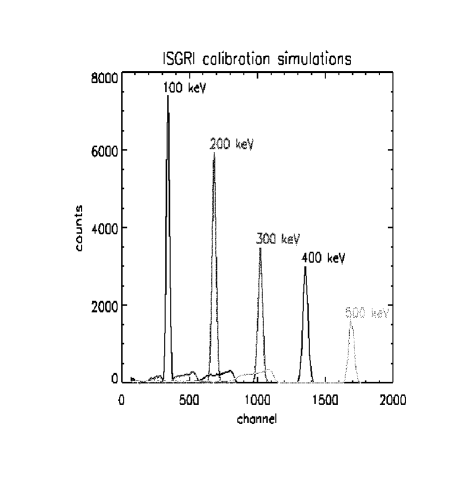
Figure 1: Simulated ISGRI response to on-axis mono-energetic sources of different energies. The spectra are binned with different factors.

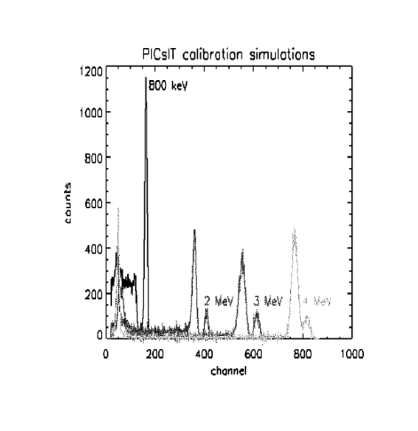
Figure 2: Simulated PICsIT response to on-axis mono-energetic sources of different energies.

The simulations clearly show the photopeak, the Compton edge and, in the case of PICsIT the backscattering peak (see Figure 3). These three features have been fitted separately with analytical functions. The photopeak required a Gaussian function, while the other two required a Gaussian plus a quadratic function.

The resulting set of parameters as a function of the energy have been then interpolated over the entire range of energies of the two instruments (see Figure 4).

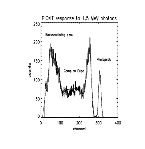
Figure 3: Simulated PICsIT response to a mono-chromatic source of 1.5 MeV photons.

Figure 4: Interpolation of the photopeak parameters of the ISGRI response.

Finally these results have been used to create two FITS files (for each detector): an RMF file containing the normalized matrix and an ARF file which contains the information about the efficiency of the instruments. These two files have been created in such a way that they are compatible with the XSPEC data analysis package (OGIP standard ver. 1992a).

The matrices have been tested with different input spectra. An example is the following: a $\sim$100mCrab, on-axis source with a power law spectrum observed for 1050 s (input parameters: photon index $\Gamma$=2, A_100keV = 9$\times$$10^{-5}$ ph cm^-2 s^-1 keV^-1). The best fit with XSPEC yielded $\Gamma$ = 1.987 $\pm$ 0.0483 , A_100keV = (8.744 $\pm$ 0.6357)$\times$$10^{-5}$ ph cm^-2 s^-1 keV^-1, Reduced $\chi^{2}$ = 0.942394. The confidence contours of the fit are presented in Figure 5.

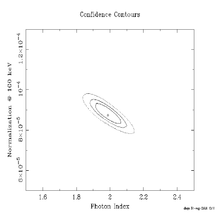
Figure 5: Confidence contours of the power law parameters for a $\sim$1000 s observation of a $\sim$100mCrab source.

3 Scientific applications

3.1 Nova Muscae (GRS 1124-684)

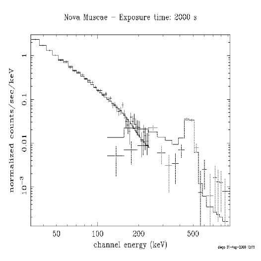
Figure 6: 2000 s IBIS simulation of Nova Muscae.

The X-ray transient GRS 1124-684 (Nova Muscae) was discovered in 1991 with the GRANAT and GINGA satellites. Measurement of its mass function during quiescence established the presence of a black hole (Remillard et al. 1992). GRS 1124-684 was observed several times by the SIGMA telescope during its outburst (Goldwurm et al. 1992). An emission feature at $\sim$500 keV was discovered during the last 13 hours of the January 20th observation.

We have simulated IBIS observations of this spectral feature, with exposure times ranging from 125 s to 15,000 s, using as input parameters the values measured by SIGMA. An example of a 2000 s simulation (see Table 1) is shown in Figure 6. The simulations show that the $\sim$500 keV feature can be appreciated ($\sim$3 $\sigma$) for observations as short as 500 s.

Table 1: IBIS simulation of Nova Muscae - Exposure time: 2000 s.

	Input parameter	Best fit result
Photon Index	2.42	2.423 $\pm$ 0.0184
Norm. at 1 keV	11.27 ph cm-2 s-1 keV-1	10.68 $\pm$ 0.741 ph cm-2 s-1 keV-1
Line energy	481 keV	483.3 $\pm$ 2 keV
Line width ($\sigma$)	23 keV	20.66 $\pm$ 0.1199 keV
Line flux	6$\times$$10^{-3}$ ph cm-2 s-1	(3.017 $\pm$ 0.242)$\times$$10^{-3}$ ph cm-2 s-1

3.2 IBIS line sensitivity

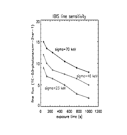
Figure 7: IBIS line sensitivity obtained from the simulations described in Section 3.2.

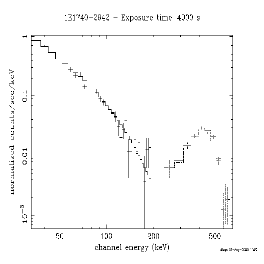
Figure 8: 4 ks IBIS simulation of 1E1740-2942.

We have performed simulations with different exposure times and spectral parameters to determine the sensitivity to detect an emission line at $\sim$ 500 keV over a continuum. Figure 7 shows the minimum exposure time that is required for a $\sim$3 $\sigma$ detection of such a feature as a function of the line flux and width ($\sigma$). The continuum used is that of Nova Muscae (see Table LABEL:table_1). A feature like that observed in 1E 1740-2942 during October 13-14 1990 with the SIGMA telescope (Bouchet et al. 1991), for example, can already be detected with an exposure time of $\sim$250 s. We have also performed some simulations of this object. The parameters, that we have used, were a Gaussian line (center = 480 keV, $\sigma$ = $\sim$100 keV, flux = 1.3$\times$$10^{-2}$ ph cm^-2 s^-1) over a comptonization continuum (kT = 27 keV, $\tau$ = 3.2). In Figure 8 we present a 4 ks simulated IBIS spectrum of 1E1740-2942.

4 Conclusions

Of course the matrices presented here, being obtained trough simulations and not by real calibration data, are intrinsically limited in their accuracy owing to the simplifications inherent to the simulator programs. Nevertheless they can be used to analyze simulated data and to obtain an estimate of the observation time required to achieve specific scientific objectives.

Future work will include the following effects that are not yet implemented in the current version:

1) Charge loss in ISGRI, caused by the different mobility of the charge/hole pairs in semiconductors;
2) Pixel disuniformity and/or gain variations;
3) Multiple interactions in PICsIT;
4) Angular dependence of the spectral response;
5) Background spatial disuniformity;

References

- [1] Bouchet L. et al., 1991, ApJ 383, L45.
- [2] Goldwurm A. et al., 1992, ApJ 389, L79.
- [3] Lei F. et al., 1999, Proc. of the Third Integral Workshop, Astro. Lett. and Communications, 39, 373.
- [4] Remillard R.A. et al., 1992, ApJ 399, L145.
- [5] Ubertini P. et al., 1999, Proc. of the Third Integral Workshop, Astro. Lett. and Communications, 39, 331.