Microstructure of the Local Interstellar Cloud and the Identification of the Hyades Cloud.

Seth Redfield JILA, University of Colorado Boulder, CO 80309 sredfiel@casa.colorado.edu Jeffrey L. Linsky JILA, University of Colorado and NIST Boulder, CO 80309 jlinsky@jila.colorado.edu

Abstract

We analyze high-resolution UV spectra of the Mg II h and k lines for 18 members of the Hyades Cluster to study inhomogeneity along these proximate lines of sight. The observations were taken by the Space Telescope Imaging Spectrograph (STIS) instrument on board the Hubble Space Telescope (HST). Three distinct velocity components are observed. All 18 lines of sight show absorption by the Local Interstellar Cloud (LIC), ten stars show absorption by an additional cloud, which we name the Hyades Cloud, and one star exhibits a third absorption component. The LIC absorption is observed at a lower radial velocity than predicted by the LIC velocity vector derived by Lallement & Bertin (1992) and Lallement et al. (1995), ( $v_{\rm predicted}(\rm LIC)-v_{\rm observed}(\rm LIC)=2.9~{}\pm~{}0.7$ km s^-1), which may indicate a compression or deceleration at the leading edge of the LIC. We propose an extention of the Hyades Cloud boundary based on previous HST observations of other stars in the general vicinity of the Hyades, as well as ground-based Ca II observations. We present our fits of the interstellar parameters for each absorption component. The availability of 18 similar lines of sight provides an excellent opportunity to study the inhomogeneity of the warm, partially ionized local interstellar medium (LISM). We find that these structures are roughly homogeneous. The measured Mg II column densities do not vary by more than a factor of 2 for angular separations of $\lesssim~{}8^{\circ}$ , which at the outer edge of the LIC correspond to physical separations of $\lesssim~{}0.6$ pc.

stars: chromospheres — ISM: atoms — ISM: clouds — ISM: structure — ultraviolet: ISM — ultraviolet: stars

1 Introduction

The morphology and physical properties of our Local Interstellar Medium (LISM) are being actively studied but are still not fully understood. Many recent high-resolution observations have uncovered hints of a complex LISM structure that have yet to be synthesized into a coherent picture. That the structure of the LISM, extending $\sim~{}250$ pc from the Sun, is not a homogeneous medium has been demonstrated by Frisch & York (1991) and by Diamond, Jewell, & Ponman (1995), from comparing measurements of H I column density ( $N_{\rm HI}$ ) with distance. In comparisons of Na I column density observations, Sfeir et al. (1999) demonstrated that there is very little cold neutral material within 50 pc of the Sun. They interpreted the rapid accumulation of Na I column density at distances $>~{}50$ pc as indicating the boundary of the Local Bubble, a superbubble cavity of hot ionized material produced by the OB star winds and supernovae of the Scorpius-Centaurus association (Frisch, 1995; Lyu & Bruhweiler, 1996). The inhomogeneous variation of H I column density measured within the Local Bubble indicates that warm, partially ionized material exists within the Local Bubble as a complex of cloudlet structures.

The simplest interpretation of the structure of the complex of warm, partially ionized material is that of individual clouds, which in this simple model would be coherent in density, velocity, temperature, and abundances. Lallement & Bertin (1992) and Lallement et al. (1995) found a coherent velocity structure for the warm gas cloud that directly surrounds the solar system. They called this cloud the Local Interstellar Cloud (LIC). The LIC velocity vector agrees with the flow of material through the heliosphere, and into the solar system, as measured by Witte et al. (1993), implying that the Sun is located inside the LIC. The LIC velocity vector has also been successful in predicting central absorption velocities for many lines of sight through the LIC. The temperature structures of different clouds in the LISM are studied by comparing the Doppler width of absorption by atoms and ions of different mass. Absorption for LIC lines of sight indicates a temperature of 8000 $\pm$ 1000 K (Linsky et al., 1993; Lallement et al., 1994; Linsky et al., 1995; Gry et al., 1995; Piskunov et al., 1997; Wood & Linsky, 1998).

Linsky et al. (2000) summarized the hydrogen and deuterium column densities through the LIC along many lines of sight toward nearby stars inferred from spectra obtained with the Goddard High Resolution Spectrograph (GHRS) and Space Telescope Imaging Spectrograph (STIS) instruments on the Hubble Space Telescope (HST) and the Extreme Ultraviolet Explorer (EUVE). Taking advantage of the constant D/H ratio in the LIC, and assuming a constant H I density in the cloud, Linsky et al. (2000) estimated the distance to the edge of the LIC for many lines of sight. Redfield & Linsky (2000) synthesized the results and were successful in fitting a quasi-spheroid structure to the observed data. This model has successfully predicted hydrogen column densities along various lines of sight (Wood et al., 2000a).

The first-order assumptions involved in the cloudlet model of the LISM may be too simplistic. Using ultra-high resolution Ca II spectra of nearby stars, Welsh, Lallement, & Crawford (1998) presented preliminary results that indicate a complex velocity structure of inhomogeneous absorption. A highly inhomogeneous, filamentary structure has already been proposed to explain abundance anomalies and the LISM velocity structure (Frisch, 1981, 1996, 2000). Shock-front destruction of dust grains can in principle account for the observed abundance anomalies, and the general LISM velocity structure appears to be consistent with the outflow of material from the Scorpius-Centaurus association.

Measurements of the degree of inhomogeneity in the LISM are needed to understand the structure and morphology of the LISM. One test of homogeneity involves a comparison of interstellar medium (ISM) parameters along similar lines of sight. For example, Frail et al. (1994) studied observations of absorption toward high-velocity pulsars in the 21-cm H I fine structure line. The high transverse velocity of these objects actually shifts the line of sight by tens of AU yr^-1. Changes in the absorption spectra indicate small-scale structure on scales of 5-100 AU. Most of these pulsars are located well outside of the Local Bubble (d $=~{}55-2650$ pc), so these inhomogeneities are most likely not associated with nearby ( $<~{}50$ pc) cloud material.

Another technique for studying similar lines of sight is to observe wide binary or multiple star systems. Watson & Meyer (1996) and Meyer & Blades (1996) have observed Na I and Ca II absorption variations for multiple systems with stellar separations of 480 to 29,000 AU. Observations of other ions dominant in the cold neutral medium (Cr II and Zn II) by Lauroesch et al. (1998) show no interstellar absorption variation, making it difficult to ascertain the nature of the variable material. However, most of these binaries are located more than 100 pc away, and may be at the edge or outside of the Local Bubble. The observed small scale structure is therefore likely produced in the cold neutral medium component of the ISM, near the boundary of the Local Bubble or beyond. Therefore, there is no evidence for significant variations in the warm, partially ionized material in the solar neighborhood along similar sight lines. Likewise, the nearest multiple star system ( $\alpha$ Cen A, $\alpha$ Cen B, and Proxima Cen), shows no sign of variations in interstellar absorption over time, or among the similar sight lines of each star (Linsky & Wood, 1996; Wood et al., 2000b). At a mean distance of 1.3 pc, the physical separations of the two $\alpha$ Cen stars is only 24 AU, while Proxima Cen is 12,000 AU away from the other two stars.

Although the inhomogeneity of the LISM is central to our understanding of the ISM, most observations to date (e.g., Na I and Ca II) have sampled primarily the cold neutral component near the boundary of the Local Bubble. There has yet to be a significant test of the homogeneity of the warm, partially ionized LISM that directly surrounds the solar system. In this paper we present observations of a sample of 18 stars in the Hyades cluster. As members of the same stellar cluster, they share similar sight lines. This data set will directly address the inhomogeneity of the LIC and other warm material in the LISM, and provide a test of our current understanding of the morphology and physical properties of the LISM. The STIS spectra are described in § 2, and we present in § 3 our determination of the interstellar parameters. In § 4, we discuss the implications of the measured interstellar parameters for the inhomogeneity of the LIC.

2 Observations

The Space Telescope Imaging Spectrograph (STIS) instrument aboard HST is described by Kimble et al. (1998) and Woodgate et al. (1998). STIS observed 18 F dwarf members of the nearby Hyades star cluster. Details regarding the observations are given in Table 1. This dataset was acquired under observing program 7389 with principal investigator E. Bohm-Vitense. All exposures were taken with the E230H grating and the 0.1” x 0.2” or 0.2” x 0.2” aperture to attain a spectral resolution of 2.6 $\rm km~{}s^{-1}$ . Within the 2674-2945 Å observed spectral range, only the Mg II h and k lines show identifiable interstellar absorption features. The S/N ratios near the peak of these lines range from 5-20.

We reduced the data acquired from the HST Data Archive using the STIS team’s CALSTIS software package written in IDL (Lindler, 1999). The reduction included assignment of wavelengths using calibration spectra obtained during the course of the observations. The ECHELLE_SCAT routine in the CALSTIS software package was used to remove scattered light. However, the scattered light contribution is negligible in this spectral range, and does not influence the uncertainties in our spectral analysis.

3 Discussion

3.1 Spectral Analysis

Figures 1a, 1b, and 1c show the Mg II h and k lines observed from the 18 Hyades stars. The vacuum rest wavelengths of the h and k lines are 2803.531 Å and 2796.352 Å, respectively. In Figures 1a, 1b, and 1c, the Mg II lines are shown with a heliocentric velocity scale, together with the best fits to the absorption by each interstellar component (dotted lines), and the total interstellar absorption convolved with the instrumental profile (thick solid lines). Although interstellar absorption is obvious for all of the lines of sight, sometimes two, and in one case (HD 28736), three velocity components are clearly visible.

All of the Hyades target stars have radial velocities $>$ 30 km s^-1. Therefore, the peaks of the Mg II h and k emission lines are shifted $>$ 30 km s^-1 to the red. Since all interstellar absorption occurs at velocities $<$ 30 km s^-1, the interstellar features appear on the blue side of the Mg II lines. This convenient placement of the interstellar absorption allows us to implement a straightforward method for estimating the missing stellar continuum across the absorption. We fit a polynomial to spectral regions just blueward and redward of the interstellar absorption. Our estimated stellar emission is shown by the thin solid lines in Figures 1a, 1b, and 1c.

Once the stellar Mg II emission line profiles have been estimated, we fit the interstellar absorption using standard techniques (cf. Linsky & Wood (1996); Piskunov et al. (1997); Dring et al. (1997)). We start with only one absorption component in the fit, and increase the number of components as the data warrant, and the quality of the fit improves. For 10 of the 18 Hyades stars adding a second component improved the $\chi^{2}$ metric significantly, while the spectral fit of only one star (HD 28736) improved significantly with the addition of a third component. While, additional weak absorption components could be present, they do not appear in the data much above the level of noise, and thereby do not significantly influence the $\chi^{2}$ metric. Therefore, we fit the spectra with the lowest number of absorption components that allow for an acceptable fit. HD 29419 indicates that additional components are not likely. Along this line of sight, the velocity difference between the LIC and Hyades Cloud is greatest, and we observe the maximum Hyades Cloud Mg II column density. Together, these two characteristics provide two well-defined and separated absorption features. Of course, the other Hyades Cloud lines of sight are not as obvious, but are satisfactorily fit by only two components. The rest wavelengths and oscillator strengths of the Mg II lines used in our fits are taken from Morton (1991), and we use Voigt functions to represent the opacity profiles of the fitted interstellar absorption. The dotted lines in Figures 1a, 1b, and 1c are the absorption line fits before convolution with the instrumental line spread function. The thick solid lines in the figures that fit the data are the final combined absorption features with the instrumental broadening applied. The instrumental line spread functions assumed in our fits are taken from Sahu et al. (1999a).

We fit both the h and k lines simultaneously in order to glean all available absorption information from the data. The factor of 2 difference in oscillator strengths between the h and k lines can be very useful in constraining the interstellar parameters, the stellar continuum level, and the number of absorption components. For example, the Mg II k line for HD 27808 is very saturated, making it difficult to determine unique values for the interstellar column density and Doppler parameter. However, the less opaque Mg II h line shows a weaker, unsaturated interstellar absorption line. Simultaneously fitting both lines allows us to determine the interstellar absorption parameters more accurately than by fitting only one of the lines. We fit each line separately as well, to see how much the parameters change, allowing us to estimate the systematic errors involved in our fits and better determine the uncertainties in the various fit parameters.

Table 3 lists the values for the interstellar absorption parameters and $1\sigma$ errors. For each absorption component there are three parameters: the central velocity ( $v$ [km s^-1]), the Doppler width ( $b$ [km s^-1]), and the Mg II column density ( $\log N_{\rm MgII}$ [ $\log$ (cm^-2)]). The central velocity corresponds to the mean projected velocity of the absorbing material along the line-of-sight to the star. If we assume that the warm partially ionized material in the solar neighborhood exists in small, homogeneous cloudlets each moving with a single bulk velocity, then each absorption component will correspond to a single cloudlet, and its velocity is the projection of its three-dimensional velocity vector. The Doppler parameter is related to the temperature ( $T$ [K]) and nonthermal velocity ( $\xi$ [km s^-1]) of the interstellar material by the following equation:

b^{2}=0.016629\frac{T}{A}+\xi^{2},

(1)

where A is the atomic weight of the element in question ( $A=24.312$ for Mg). Because of the large atomic weight of Mg, the Doppler parameter is more sensitive to changes in turbulent velocity than temperature. The Mg II column density is a measure of the amount of material along the line of sight to the star. If we assume homogeneous cloudlets with constant density, the column density will be directly proportional to the cloud thickness. We have identified three separate velocity components, and therefore three individual cloudlets, along the line of sight to the Hyades stars. Columns 2-4 of Table 3 list the interstellar parameters for velocity components associated with the LIC, columns 5-7 list interstellar parameters for the newly identified Hyades Cloud, and columns 8-10 list the same for the third velocity component. The velocity spatial structure is discussed in Section 3.3, the Doppler parameter spatial structure is discussed in Section 3.4, and the column density spatial structure is discussed in Section 3.5.

3.2 Spatial Analysis

The spectra shown in Figures 1a, 1b, and 1c clearly show several distinct absorption features. Because the lines of sight to all of our targets are in close proximity, we expect that many of these absorption features should sample the same interstellar cloudlet structure. If the lines of sight to our targets pass through the same cloud structures, then the inferred interstellar parameters ( $b,v,N_{\rm MgII}$ ) should be similar, and the projected spatial structure is probably continuous. The presence of distinct boundaries where the absorption by a cloud is present in one star but not in close neighbors would indicate that the cloud has a sharp boundary. Furthermore, similar interstellar parameters for the cloud inferred from adjacent lines of sight would imply that a cloud is, to first-order, homogeneous.

In Table 3 we have grouped the absorption features into three separate cloudlets. The first, present in the spectra of all 18 target stars, has velocities ranging from 20-24 km s^-1 and is associated with the Local Interstellar Cloud (LIC). The second cloudlet, clearly present in the spectra of 10 target stars, has velocities ranging from 12-17 km s^-1. We now call this structure the Hyades Cloud (HC). The third cloudlet, only detected toward one target star (HD 28736), has a velocity $\sim$ –4 km s^-1. In Figure 2 we plot the spatial distribution of the Hyades target stars, and the rough outlines of the Hyades Cloud and the third cloudlet. Because of the limited spatial sampling, the true extent of these clouds is not yet known. However, the dashed lines represent the positions between adjacent target stars, where the location of the boundary is reasonably well defined. The consistency of the interstellar parameters determined from the spectra of the 10 target stars, and the contiguous spatial projection, implies that the Hyades Cloud is in fact a coherent body with a roughly homogeneous structure.

The location of these clouds along the line of sight is a more difficult question to answer. Because absorption due to the LIC has been observed for many other stars, Redfield & Linsky (2000) were able to calculate a three-dimensional model of the LIC. Based on this model, the LIC is expected to extend $\sim$ 5.8 pc in the direction of the Hyades. The Hyades Cloud could, therefore, be located anywhere from the edge of the LIC to the Hyades Cluster, perhaps surrounding the target stars themselves. Figure 3 shows the measured Mg II column density as a function of distance. If the Hyades Cloud actually surrounds the Hyades stars, we would expect to see a trend of increasing Mg II column density with distance. We see no such trend, and therefore conclude that the LIC and Hyades clouds are both located, in their entirety, in front of the target stars. The location of the Hyades Cloud ( $d_{HC}$ ) is therefore limited to $5.8~{}\rm{pc}\leq d_{HC}\leq 41.2~{}\rm{pc}$ . The mean column density for each cloud is given by the dashed line. For the LIC the mean Mg II column density is $\log N_{\rm MgII}\sim\ 12.63~{}\log$ (cm^-2). The Hyades Cloud has a mean Mg II column density of $\log N_{\rm MgII}\sim\ 12.13~{}\log$ (cm^-2). The factor of 3 lower mean column density implies that the Hyades Cloud is either thinner or less dense than the LIC. If we assume that the Hyades Cloud has similar physical characteristics to the LIC, including a similar H I density ( $n_{\rm HI}=0.10~{}\rm{cm}^{-3}$ ) and Mg II depletion (–1.1 dex), then we estimate the thickness of the Hyades Cloud to be $\sim\ 1.8~{}\rm pc$ .

3.3 Velocity Structure

Since we can fit the LISM absorption successfully with Voigt profiles, we presume that the medium along a given line of sight for each cloud is moving at a single bulk velocity, with symmetric thermal and turbulent motions. The measured central velocity and 1 $\sigma$ error bars for each absorption feature is given in Table 3. The velocities of absorption features that we identify with the LIC are given in column 2, those that we identify with the Hyades Cloud are given in column 5, and the third component is given in column 8.

If we assume that each cloudlet structure in the LISM is moving with a single-valued bulk velocity, then we can calculate a unique velocity vector for each individual cloud. Due to the small number of lines of sight previously sampled, unique velocity vectors have only been calculated for two clouds: the LIC and the Galactic (G) Cloud (Lallement et al., 1995). In the heliocentric rest frame, the LIC, in which the Sun is embedded, is flowing toward Galactic coordinates $l=186^{\circ}$ and $b=-16^{\circ}$ at a speed of $25.7~{}\pm~{}0.5$ km s^-1 (Witte et al., 1993; Lallement & Bertin, 1992). Using this vector we compute the projected LIC velocities ( $v_{\rm{LIC}}$ ), for the lines of sight toward our Hyades stars. In Table 4 the predicted velocity values are given in column 2, and the observed central velocities associated with the LIC are given in column 3. We observe LIC absorption in all 18 Hyades target stars, but the observed velocity values are systematically lower than the predicted values. The mean difference ( $v_{\rm predicted}(\rm LIC)-v_{\rm observed}(\rm LIC)$ ) is $2.9~{}\pm~{}0.7$ km s^-1. Two plausible explanations for this discrepency are that unresolved blended absorption features are offsetting our central velocity fits, or that the calculated LIC velocity vector is inaccurate for this region of the sky. The presence of the Hyades Cloud absorption (typically $\sim\ 7.8$ km s^-1 from the observed LIC velocity) does not seem to affect the LIC velocity measurements. The 10 target stars that show Hyades absorption, often blended with the LIC absorption, have a mean LIC velocity difference similar to the overall mean ( $v_{\rm predicted}(\rm LIC)-v_{\rm observed}(\rm LIC)=2.7\pm 0.8$ km s^-1), as do those without Hyades absorption features ( $v_{\rm predicted}(\rm LIC)-v_{\rm observed}(\rm LIC)=3.1\pm 0.6$ km s^-1). The LIC velocity vector determined by Lallement & Bertin (1992) used nine lines of sight distributed over the entire sky. The nearest target to the Hyades stars in their sample is $\eta$ Aur, about 25^∘ away, with absorption at $23.0~{}\pm~{}1.5$ km s^-1. Now that many more lines of sight have been studied since the Lallement & Bertin (1992) determination of the LIC velocity vector, a revision of the vector could bring the Hyades velocities into better agreement. However, the $2.9~{}\pm~{}0.7$ km s^-1 discrepancy between the predicted and the observed projected LIC velocity cannot be accounted for by small corrections in the LIC velocity vector direction or magnitude. Therefore, a single bulk velocity flow may not be realistic throughout the whole LIC. Note that the leading edge of the LIC, moving with a velocity of 25.7 km s^-1 along the line of sight towards $l=186^{\circ}$ and $b=-16^{\circ}$ , is very near to the lines of sight to the Hyades stars. Our observations of slightly slower velocities may indicate a compression and deceleration at the leading edge of the LIC. We will address these questions in a future paper.

Ten of the 18 Hyades Stars show a second absorption feature in the velocity range of 12-17 km s^-1 with a mean value of 14.8 km s^-1. We have identified what we now call the Hyades Cloud based on the similar absorption velocities measured for these ten lines of sight. Because the Hyades stars cover a small area of the sky, and do not show a clear trend in velocity across the sample area, it is not yet feasible to calculate a velocity vector. If the kinematic structure of the LISM is coherently organized, then the direction of the Hyades Cloud velocity vector is expected to be similar to the direction of the LIC velocity vector. The G Cloud and the LIC vectors, for example, are very similar (Lallement et al., 1995). Therefore, we anticipate that other nearby targets with lines of sight that also traverse the Hyades Cloud, will have absorption at velocities $<$ 5 km s^-1 from the measured mean value of Hyades absorption at 14.8 km s^-1. Figure 4 shows an expanded view of the Hyades region in Galactic coordinates with other nearby stars plotted along with the Hyades stars. The Hyades sample is plotted as circles, while other targets that have Mg II absorption detected by HST are plotted as squares, and targets that have Ca II absorption observed with ground-based telescopes are plotted as triangles. Only high resolution data (R $=\lambda/\Delta\lambda\gtrsim 100,000$ ) are included in these samples. The HST targets are listed in Table 5 and the Ca II targets are listed in Table 6. We have separated those stars that show absorption in the velocity range from 10-20 km s^-1 from those that do not. In Figure 4, those targets that show absorption at a velocity consistent with the Hyades Cloud are plotted as filled symbols, while those that do not are plotted as open symbols. This provides a tentative means for establishing the boundary of the Hyades Cloud. Clearly the Hyades Cloud does not extend far to the Galactic North-East (upper left in the figure), due to the large number of objects that do not show Mg II or Ca II absorption at the Hyades Cloud velocity. Nor does the Hyades Cloud extend far to the Galactic South-West (lower right in the figure), as $\epsilon$ Eri and 40 Eri A do not show any Hyades Cloud absorption. It appears that the Hyades Cloud structure may extend almost linearly across the sky from Galactic South-East to Galactic North-West, in a filamentary structure. Definitive proof of Hyades Cloud absorption can only be made by self-consistent measurements of a velocity vector, cloud temperature, and elemental abundances. As this requires high resolution spectra in the 1200-1350 Å region, which are not yet available, this task is beyond the scope of this paper, and we simply provide a tentative boundary based on similarity of absorption velocity. The large apparent size of the Hyades Cloud suggests that it is probably located nearby, just beyond the LIC. The fact that Sirius, only 2.6 pc away, may be a member of the Hyades Cloud, supports the indication that the Hyades Cloud is nearby. The absorption at the Hyades Cloud velocity towards Sirius was identified by Lallement et al. (1994) as the Blue Cloud.

In Figure 4, a tentative boundary (the dotted-dashed line) is given for the third component that is observed towards HD 28736. No other nearby stars show absorption at a velocity similar to the third component velocity (–4.3 km s^-1). Therefore, this third component cloud is limited to a small region on the sky, indicating that it is likely located farther away than the Hyades Cloud.

3.4 Temperature and Turbulent Structure

The observed value of the Doppler parameter ( $b$ ) is a measure of the temperature ( $T$ ) and turbulent velocity ( $\xi$ ). The relationship is provided in Equation 1. Because of its relatively large atomic weight, magnesium’s Doppler parameter is primarily due to turbulence or unresolved clouds along the line of sight. The measured Doppler parameter and 1 $\sigma$ error bars for each absorption feature are given in Table 3. If we assume that the temperature and turbulent structure in a cloud are relatively constant, the Doppler parameters should be equal. For the LIC absorption component, all 18 lines of sight are in good agreement regarding the Doppler parameter. The mean b-value for the LIC is $b_{\rm LIC}~{}3.5~{}\pm$ 0.6 km s^-1. If we assume a LIC temperature of $T_{\rm LIC}~{}\sim~{}8000~{}\pm~{}1000~{}\rm{K}$ (Piskunov et al., 1997; Linsky et al., 1995; Lallement et al., 1994; Witte et al., 1993), then the turbulent velocity in this region of the LIC is $\xi_{\rm LIC}~{}\sim~{}2.6~{}\pm~{}0.8$ km s^-1. This value is larger than values calculated for the LIC along other lines of sight (Piskunov et al., 1997; Lallement et al., 1994; Linsky et al., 1995), but not for the LISM in general (Lallement et al., 1994; Wood, Linsky, & Zank, 2000). Since the mean $b_{\rm LIC}$ is identical for those lines of sight with and without additional Hyades absorption, we do not believe that unresolved blends are compromising our measurements of the turbulence values.

The weaker, blended Hyades absorption component permits us to determine the Doppler parameter but with lower precision. The 1 $\sigma$ error bars are larger owing to the absorption being a blended and weaker line. The mean Mg II b-value for the Hyades component is $b_{\rm HC}=2.8~{}\pm$ 0.9 km s^-1, indicating a lower temperature cloud or a less turbulent structure than the LIC. In Table 5, the other Mg II observations of nearby targets give b-values that agree within the errors of the mean Hyades sample b-value. This is an additional indication that these lines of sight traverse the same cloud structure.

Many of the stars observed by HST and listed in Table 5 that show Hyades Cloud absorption in Mg II also show Hyades Cloud absorption in other atomic lines. Observations of absorption in many lines allow the temperature and turbulent velocity in the cloud to be measured. These parameters are listed in columns 9 and 10 of Table 5. The measured b-values of Mg II and H I Hyades Cloud absorption along the line of sight to HR 1099 do not permit a unique determination of the temperature or turbulent velocity. Observations of Hyades Cloud absorption in other atomic lines are needed to satisfactorily determine these two quantities along this line of sight. Likewise, the complicated LISM absorption spectra seen in observations of $\beta$ CMa led Dupin & Gry (1998) to force a Hyades Cloud absorption component fixed by the ISM parameters measured towards $\epsilon$ CMa. Although the absorption toward $\beta$ CMa is therefore consistent with Hyades Cloud absorption, the $\beta$ CMA data provide no additional information on the physical properties of the Hyades Cloud. Therefore, the interstellar parameters for $\beta$ CMa are not listed in Table 5, and those interstellar parameters listed for HR 1099 should be given low weight.

3.5 Column Density Structure

The observed Mg II column density indicates the number of Mg⁺ ions along the line of sight. If we assume a homogeneous medium with a constant density, the column density is directly proportional to the distance that the line of sight traverses through the cloud. The measured Mg II column densities and 1 $\sigma$ error bars for each absorption feature are given in Table 3. Column 4 lists the Mg II column density associated with the LIC. Figure 5 shows a crude contour plot of the LIC Mg II column density. A negative gradient in column density is clearly evident from Galactic North-East to Galactic South-West. The target with the maximum column density is HD 21847 ( $l=156.2$ and $b=-16.6$ ) and the minimum column density through the LIC is in the line of sight of HD 26784 ( $l=182.4$ and $b=-27.9$ ). The gradient is fairly smooth between these two stars. Redfield & Linsky (2000) developed a three-dimensional model of the macroscopic structure of the LIC using 32 lines of sight, and assuming a homogeneous, constant density cloud structure. Figure 5 shows the H I column density predicted from their model as shading. The model shows a gradient in H I column density that is similar to what is seen in Mg II over the same region. The predicted values of the H I column density for the lines of sight to the Hyades stars are listed in column 4 of Table 4. Although the depletion of Mg may change somewhat for different lines of sight through the LIC (see the next section), we do not expect the Mg depletion to change drastically over small distances. Our result that the two column densities are indeed found to be consistent is an excellent check for the Redfield & Linsky (2000) LIC model, and for the quality of the Hyades analysis.

As discussed in Section 3.2, the mean Mg II column density through the Hyades Cloud is more than a factor of 3 smaller than the Mg II column density through the LIC. The measured values of the Hyades Cloud Mg II column density are listed in column 7 of Table 3. Due to the random error associated with the low S/N of the observations, and the systematic errors created by the uncertainty in the continuum and the tendency for the Hyades Cloud absorption to be blended with the LIC absorption, we estimate that the minimum Mg II column density that could be detected to be $\log~{}N_{\rm MgII}=11.5~{}\log(\rm{cm}^{-2})$ . This value includes the random errors of measurement and our estimate of the more important systematic errors. The upper limit of the Mg II column density for our Hyades Cloud nondetections is therefore $\log~{}N_{\rm MgII}=11.5~{}\log(\rm{cm}^{-2})$ . Like the LIC, the Hyades Cloud shows a smooth gradient in column density with position on the sky. Figure 6 shows the Mg II column density contours for those lines of sight that show absorption greater than our detection limit, consistent with Hyades Cloud velocities. The tentative outline of the Hyades Cloud from Figure 2 is also provided. The maximum Mg II column density is exhibited by the isolated star HD 29419, and the minimum detected Mg II column density is for the line of sight to HD 27848, located close to the edge of the Hyades Cloud at $l=178.6$ and $b=-22.0$ . The Mg II column density gradient clearly decreases from the interior of the Hyades Cloud towards the edge near HD 27848. Other nearby stars that show absorption at velocities similar to the Hyades show Mg II column densities consistent with those found in the Hyades sample itself. These values are given in Table 5, and provide additional evidence that these lines of sight traverse the same physical cloud as the Hyades sample.

3.5.1 Mg II Depletion

The gas-phase abundance of elements in the LISM is an important physical parameter for our understanding of the structure of the LISM. The analysis of Lallement et al. (1994) demonstrated that Mg II is the dominant ionization state of magnesium in the LISM. It has been found that the gas-phase abundance of Mg II can vary considerably in the LISM (Piskunov et al., 1997; Dring et al., 1997). Depletion is defined by the equation,

D(\rm{Mg})=\log\left[\frac{N_{\rm MgII}}{N_{\rm HI}}\right]-\log\left[\frac{\rm{Mg}}{\rm{H}}\right]_{\odot},

(2)

where the solar abundance of magnesium to hydrogen is $\log(\rm{Mg/H})_{\odot}=-4.41$ (Anders & Grevesse, 1989). Note that these depletion values assume that all hydrogen in the LISM is neutral. The ionization state of the LISM is uncertain, but it is likely that nearly half of the hydrogen is ionized (Wood & Linsky, 1997; Lallement et al., 1994). In this case, the depletion values calculated from Equation 2 may be too large by 0.3 dex or more. Depletion values derived by Piskunov et al. (1997) and Dring et al. (1997) imply a LIC depletion value for magnesium of D(Mg) $=~{}-1.1~{}\pm~{}0.2$ . This is similar to the depletion D(Mg) $=~{}-0.89~{}\pm~{}0.05$ obtained for the warm cloud in the line of sight to $\zeta$ Oph (Savage & Sembach, 1996).

The Hyades sample unfortunately does not have corresponding spectra of H I (1216 Å), and therefore does not allow for an independent measure of the hydrogen column density and magnesium depletion. However, the Redfield & Linsky (2000) LIC model provides predictions of the H I column densities through the LIC for any line of sight. In Table 4 the predicted LIC hydrogen column densities are listed in column 4, and the measured LIC Mg II column densities, as taken from Table 3, are listed in column 5. The calculated depletions are listed in column 6. The Mg depletions range from $D(\rm{Mg})=-0.76~{}\pm~{}0.37$ to $D(\rm{Mg})=-1.32~{}\pm~{}0.13$ . Therefore all of the Hyades stars are consistent with the canonical value of LIC depletion, $D(\rm{Mg})=-1.1~{}\pm~{}0.2$ . This provides further confirmation that not only do the predicted H I column densities have a gradient similar to that of the measured Mg II column densities, but the difference between the two provides a reasonable estimate of the magnesium depletion.

The magnesium depletions in the Hyades Cloud measured by HST observations of nearby stars are listed in column 11 of Table 5. There is no clear trend among the magnesium depletion values, but they are roughly similar to the LIC value of $D(\rm{Mg})=-1.1~{}\pm~{}0.2$ . We note that the two stars with values of D(Mg) furthest from the LIC value, HR 1099 and $\epsilon$ CMa, have three or more velocity components in their lines of sight and therefore, the hydrogen column density and magnesium depletion are difficult to measure for the Hyades Cloud component.

4 Homogeneity in the LISM

The close proximity of the lines of sight to the Hyades stars provides an excellent opportunity to investigate the small-scale microstructure of warm interstellar clouds. Due to the large number of targets observed in the Hyades sample (18), and the small angular distance between them, there are large numbers of unique pairs with which to compare observed ISM parameters. Because the LIC is observed in all 18 targets, there are 153 unique pairings of targets varying in angular distance from $0.6^{\circ}$ to $33.2^{\circ}$ . Figure 7 shows the distribution of angular distances of the Hyades stars in $1^{\circ}$ bins. The left panel gives the distribution for the LIC, and it is clear that the vast majority of star pairings are less than $10^{\circ}$ away from each other. The same is true for the Hyades Cloud, as shown in the right panel of Figure 7. However, there are only 45 unique pairs for the 10 stars with Hyades Cloud absorption. The Hyades Cloud distribution of angular separations range from $1.0^{\circ}$ to $17.8^{\circ}$ .

We compare the observed Mg II column density for the LIC and the Hyades Cloud as a function of angular separation for each individual pairing. This comparison should provide some insight into the density inhomogeneity of the LISM. If there are large inhomogeneities, proximate lines of sight should not show similar column densities. In fact, we find that close lines of sight do show similar Mg II column densities. Figure 8 shows the difference in the observed Mg II column density for all pairings as a function of angular separation. The closest pairs in fact show excellent agreement in observed column densities. The top panel displays the observed Mg II column densities of the LIC for all 18 target stars. The bottom panel displays the observed Mg II column densities for the ten stars that show Hyades Cloud absorption. The similar values of $N_{\rm MgII}$ for the closest pairs indicates that the LIC and Hyades Cloud are in fact roughly homogenous. For the LIC, we have some indication of the distance to the edge of the cloud from a model based on previous observations of 32 lines of sight. Linsky et al. (2000) presented a methodology for calculating the distance to the edge of the LIC, using high resolution observations of deuterium absorption and assuming constant D/H ratio in the LIC. Redfield & Linsky (2000) used this technique to calculate distances to the edge of the LIC and to fit a three-dimensional model of the shape of the LIC. We use these estimates to the edge of the LIC to calculate physical separations at the edge of the LIC for different sight lines from the angular separations of the Hyades stars. In the top panel of Figure 8, the top axis is this distance scale in parsecs. The lines of sight of the very closest pairs of targets, which show excellent agreement, are on the order of 0.05-0.1 pc away from each other at the edge of the LIC, corresponding to separations of (1-2) $\times 10^{4}$ AU. One would not be surprised to see differences in column density to increase with increased distance, due to the macroscopic characteristics of the cloud, but it is important to determine whether the column densities change smoothly or stocastically with increasing angular separations. We have indicated where a factor of two in $\Delta~{}N_{\rm MgII}$ occurs in Figure 8. The change in column density for pairs of targets does not consistently exceed a factor of 2 until angular distances $\gtrsim~{}8^{\circ}$ or physical distances of $\gtrsim$ 0.6 pc are obtained. The transition to larger $\Delta~{}N_{\rm MgII}$ for pairs of stars seems to occur smoothly.

In the top panel of Figure 8 we also include the change in H I column density, $\Delta~{}N_{\rm HI}$ , as predicted by the Redfield & Linsky (2000) macroscopic model of the LIC. These calculations are displayed by the cross-hatch symbols ( $\times$ ). Clearly, the changes in the predicted H I column density between lines of sight to the Hyades stars are smaller than those of the measured Mg II column density. This indicates that the LIC, as measured by the Mg II column densities of this Hyades sample, is more inhomogeneous than the model. The most likely explanation is that the LIC model is undersampled, and requires many more lines of sight in order to resolve the column density flucuations. Our sample indicates that at angular separations of $\lesssim~{}8^{\circ}$ the measured column densities in the LIC do not change by more than a factor of two.

We can also study the inhomogeneity of the Doppler parameter. In Section 3.4 we discussed how the Doppler parameter is related to the temperature and turbulent velocity structure. With the many lines of sight to the Hyades stars, we can question whether the LIC and the Hyades Cloud have constant temperatures and turbulent velocities, or whether these quantities change at boundaries or interfaces. In Figure 9 we display the difference in the Doppler parameter for all pairs of stars for both the LIC and the Hyades Cloud. Clearly, the Hyades Cloud shows larger error bars due to the weak and blended absorption lines. The LIC, on the other hand, has relatively small error bars. There appears to be a distinct contrast in the difference of Mg II column density and Doppler parameter data. Whereas the Mg II column density differences show a gradual increase in difference with increasing distance, the Doppler parameter differences do not show any trend with distance, but rather a constant difference of $\sim~{}1$ km s^-1 for all distances, consistent with the uncertainties in the measurements. It is possible that the spectral resolution of our observations is not high enough to adequately determine the Doppler parameter with great enough precision to detect variations in $b$ . However, if we are successfully resolving and fitting the Doppler parameter for the observed absorption features, this behavior of the Doppler parameter may indicate that there are no large gradients in temperature or turbulent velocity.

5 Conclusions

We have analyzed Mg II h and k absorption features in HST/STIS spectra for 18 members of the Hyades Cluster. Our findings are summarized as follows:

1.

Three velocity components are observed along the lines of sight toward the Hyades Cluster. All stars show absorption that is consistent with the LIC at $\gtrsim~{}20$ km s^-1. Ten of the 18 stars exhibit a secondary component at radial velocities of 12-16 km s^-1. One star (HD 28736) shows absorption of a third component at a velocity of $-4.3$ km s^-1.
2.

The observed radial velocities associated with the LIC absorption are lower than those predicted by the LIC velocity vector (Lallement & Bertin, 1992; Lallement et al., 1995) by $2.9~{}\pm~{}0.7$ km s^-1. The direction to the Hyades Cluster is also roughly the direction of the leading edge of the LIC, so the lower velocities may indicate a compression or deceleration of material at the leading edge of the LIC.
3.

The Hyades Cloud appears to extend beyond the field of view of the Hyades, as other nearby lines of sight show absorption at similar velocities. We have collected data from previous HST observations and ground-based Ca II observations. The indicated structure of the Hyades Cloud is more filamentary in nature than that inferred for the LIC.
4.

The large number of proximate lines of sight provides a unique opportunity to investigate the inhomogeneity of the LISM, and in particular individual clouds such as the LIC. We find that the range in Mg II column densities does not exceed a factor of two for angular separations of $\lesssim~{}8^{\circ}$ . Linsky et al. (2000) and Redfield & Linsky (2000) provide estimates of the distance to the edge of the LIC. With these estimates, the angular separations of $\lesssim~{}8^{\circ}$ correspond to physical distances of $\lesssim~{}0.6$ pc or $\lesssim~{}10^{5}$ AU at the edge of the LIC.

The authors would like to thank B. Wood for useful discussions and insightful comments regarding this work. We would also like to thank C. Gry for sending the results of O. Dupin’s analysis of the

\zeta

CMa line of sight. We thank the anonymous referee for their careful reading and helpful comments. This research is supported by NASA grants NGT5-50242 and S-56500-D to the University of Colorado at Boulder.

References

Anders & Grevesse (1989) Anders, E., & Grevesse, N. 1989, Geochim. Cosmochim. Acta, 53, 197
Crawford et al. (1998) Crawford, I. A., Lallement, R., & Welsh, B. Y. 1998, MNRAS, 300, 1181
Diamond, Jewell, & Ponman (1995) Diamond, C. J., Jewell, S. J., & Ponman, T. J. 1995, MNRAS, 274, 589
Dring et al. (1997) Dring, A. R., Linsky, J. L., Murthy, J., Henry, R. C., Moos, W., Vidal-Madjar, A., Audouze, J., & Landsman, W. 1997, ApJ, 488, 760
Dupin (1998) Dupin, O. 1998, Ph.D. thesis, University of Paris
Dupin & Gry (1998) Dupin, O., & Gry, C. 1998, A&A, 335, 661
Frail et al. (1994) Frail, D. A., Weisberg, J. M., Cordes, J. M., & Mathers, C. 1994, ApJ, 436, 144
Frisch (1981) Frisch, P. C. 1981, Nature, 293, 377
Frisch (1995) Frisch, P. C. 1995, Space Sci. Rev., 72, 499
Frisch (1996) Frisch, P. C. 1996, Space Sci. Rev., 78, 213
Frisch (2000) Frisch, P. C. 2000, J. Geophys. Res., 105, 10279
Frisch & York (1991) Frisch, P. C., & York, D. G. 1991, in The First Berkeley Colloquium on Extreme Ultraviolet Astronomy, Extreme Ultraviolet Astronomy, ed. R. F. Malina & S. Bowyer, (New York: Pergamon Press), 322
Gry et al. (1995) Gry, C., Lemonon, L., Vidal-Madjar, A., Lemoine, M, & Ferlet, R. 1995, A&A, 302, 497
Gry & Jenkins (in press) Gry, C., & Jenkins, E. B. 2000, A&A, in press
Hébrard et al. (1999) Hébrard, G., Mallouris, C., Ferlet, R., Koester, D., Lemoine, M., Vidal-Madjar, A., & York, D. 1999, A&A, 350, 643
Kimble et al. (1998) Kimble, R. A. et al. 1998, ApJ, 492, L83
Lallement & Bertin (1992) Lallement, R., & Bertin, P. 1992, A&A, 266, 479
Lallement et al. (1994) Lallement, R., Bertin, P., Ferlet, R., Vidal-Madjar, A., & Bertaux, J. L. 1994, A&A, 286, 898
Lallement & Ferlet (1997) Lallement, R., & Ferlet, R. 1997, A&A, 324, 1105
Lallement et al. (1995) Lallement, R., Ferlet, R., Lagrange, A. M., Lemoine, M., & Vidal-Madjar, A. 1995, A&A, 304, 461
Lauroesch et al. (1998) Lauroesch, J. T., Meyer, D. M., Watson, J. K., & Blades, J. C. 1998, ApJ, 507, L89
Lindler (1999) Lindler, D. 1999, CALSTIS Reference Guide (Greenbelt: NASA/LASP)
Linsky et al. (1993) Linsky, J. L., et al. 1993, ApJ, 402, 694
Linsky et al. (1995) Linsky, J. L., Diplas, A., Wood, B. E., Brown, A., Ayres, T. R., & Savage, B. D. 1995, ApJ, 451, 335
Linsky et al. (2000) Linsky, J. L., Redfield, S., Wood, B. E., & Piskunov, N. 2000, ApJ, 528, 756
Linsky & Wood (1996) Linsky, J. L., & Wood, B. E. 1996, ApJ, 463, 254
Lyu & Bruhweiler (1996) Lyu, C.-H., & Bruhweiler, F. C. 1996, ApJ, 459, 216
Meyer & Blades (1996) Meyer, D. M., & Blades, J. C. 1996, ApJ, 464, L179
Morton (1991) Morton, D.C. 1991, ApJS, 77, 119
Perryman et al. (1997) Perryman, M. A. C., et al. 1997, A&A, 323, L49
Perryman et al. (1998) Perryman, M. A. C., et al. 1998, A&A, 331, 81
Piskunov et al. (1997) Piskunov, N., Wood, B. E., Linsky, J. L., Dempsey, R. C., & Ayres, T. R. 1997, ApJ, 474, 315
Redfield & Linsky (2000) Redfield, S., & Linsky, J. L. 2000, ApJ, 534, 825
Sahu et al. (1999a) Sahu, K. C., et al. 1999a, STIS Instrument Handbook (Baltimore: STScI)
Sahu et al. (1999b) Sahu, M. S., et al. 1999b, ApJ, 523, L159
Savage & Sembach (1996) Savage, B. D., & Sembach, K. R. 1996, ARA&A, 34, 279
Sfeir et al. (1999) Sfeir, D. M., Lallement, R., Crifo, F., & Welsh, B. Y. 1999, A&A, 346, 785
Vallerga et al. (1993) Vallerga, J. V., Vedder, P. W., Craig, N., & Welsh, B. Y. ApJ, 411, 729
Welsh, Lallement, & Crawford (1998) Welsh, B. Y., Lallement, R., & Crawford, I. 1998, in Lecture Notes in Physics 506, The Local Bubble and Beyond, ed. D. Breitschwerdt, M. J. Freyberg, & J. Trümper (Berlin: Springer), 37
Welty et al. (1996) Welty, D. E., Morton, D. C., & Hobbs, L. M. 1996, ApJS, 106, 533
Witte et al. (1993) Witte, M., Rosenbauer, H., Banaszkewicz, M., & Fahr, H. 1993, Adv. Space Res., 13, 121
Watson & Meyer (1996) Watson, J. K., & Meyer, D. M. 1996, ApJ, 473, L127
Wood et al. (2000a) Wood, B. E., Ambruster, C. W., Brown, A., & Linsky, J. L. 2000a, ApJ, 542, 411
Wood & Linsky (1997) Wood, B. E., & Linsky, J. L. 1997, ApJ, 474, L39
Wood & Linsky (1998) Wood, B. E., & Linsky, J. L. 1998, ApJ, 492, 788
Wood et al. (2000b) Wood, B. E., Linsky, J. L., Müller, H.-R., Zank, G. P. 2000b, ApJ, in press
Wood, Linsky, & Zank (2000) Wood, B. E., Linsky, J. L., & Zank, G. P. 2000, ApJ, 537, 304
Woodgate et al. (1998) Woodgate, B. E., et al. 1998, PASP, 110, 1183

Table 1: Summary of STIS Observations

HD	Exposure	Date	S/N	S/N
#	Time		Mg II k	Mg II h
	(s)		(2796.352 Å)	(2803.531 Å)
21847	180	1999 Jan 26	10	07
26345	144	1999 Jan 09	09	08
26784	288	1999 Aug 03	18	14
27561	120	1998 Nov 07	11	09
27808	312	1999 Feb 02	19	15
27848	144	1999 Feb 10	08	07
28033	288	1999 Jul 31	06	05
28205	240	1999 Feb 04	15	11
28237	16950	1998 Dec 23	16	11
28406	240	1998 Nov 20	10	09
28483	180	1998 Nov 08	11	09
28568	144	1998 Nov 08	08	07
28608	240	1998 Nov 07	13	10
28736	144	1999 Jan 14	09	07
29225	240	1998 Oct 26	12	10
29419	288	1998 Nov 05	18	14
30738	240	1998 Nov 07	12	09
31845	150	1998 Nov 08	09	07

Table 2: Properties of Hyades Stars

HD	Spectral	$m_{\rm V}$	$v_{\rm R}$ ^a^aTaken from Perryman et al. (1998), see references within.	$l$	$b$	distance ^b^b $Hipparcos$ distances (Perryman et al., 1997).	$v_{\rm{LIC}}$ ^c^cPredicted projected LIC velocity from Lallement & Bertin (1992).	$\log N_{\rm{HI}}$ (LIC)^d^dPredicted hydrogen column density from Redfield & Linsky (2000).
#	Type		(km s^-1)	(^∘)	(^∘)	(pc)	(km s^-1)	$\log(\rm cm^{-2})$
21847	F8V	7.3		156.2	–16.6	48.9	22.6	18.31
26345	F6V	6.6	+37.1	175.2	–23.6	43.1	25.1	18.23
26784	F8V	7.1	+38.5	182.4	–27.9	47.4	25.1	18.05
27561	F5V	6.6	+39.2	180.4	–24.3	51.4	25.3	18.14
27808	F8V	7.1	+38.9	174.8	–19.1	40.9	25.2	18.23
27848	F6V	7.0	+40.1	178.6	–22.0	53.4	25.4	18.18
28033	F8V	7.4	+38.8	175.4	–18.9	46.4	25.3	18.23
28205	F8V	7.4	+39.3	180.4	–22.4	45.8	25.4	18.15
28237	F8V	7.5	+40.2	183.7	–24.7	47.2	25.4	18.07
28406	F6V	6.9	+38.6	178.8	–20.6	46.3	25.4	18.18
28483	F6V	7.1	+38.0	177.3	–19.2	50.2	25.4	18.21
28568	F5V	6.5	+40.9	180.5	–21.4	41.2	25.5	18.15
28608	F5V	7.0	+41.4	185.1	–24.7	43.6	25.4	18.06
28736	F5V	6.4	+39.8	190.2	–27.6	43.2	25.2	18.00
29225	F5V	6.6	+33.7	181.6	–20.5	43.5	25.6	18.14
29419	F5V	7.5	+39.9	176.0	–15.6	44.2	25.3	18.22
30738	F8V	7.3	+42.7	183.5	–17.6	51.8	25.7	18.13
31845	F5V	6.8	+42.5	185.1	–16.0	43.3	25.7	18.12

Table 3: Fit Parameters for the Mg II Interstellar Components

HD	$v$	$b$	$\log N_{\rm MgII}$	$v$	$b$	$\log N_{\rm MgII}$	$v$	$b$	$\log N_{\rm MgII}$	$\chi_{\nu}^{2}$
	LIC Component			Hyades Cloud Component			Third Component
#	(km s^-1)	(km s^-1)	$\log(\rm cm^{-2})$	(km s^-1)	(km s^-1)	$\log(\rm cm^{-2})$	(km s^-1)	(km s^-1)	$\log(\rm cm^{-2})$
21847	21.1 $\pm$ 0.3	2.7 $\pm$ 1.0	13.14 $\pm$ 0.37							1.16
26345	21.1 $\pm$ 0.5	3.8 $\pm$ 0.7	12.65 $\pm$ 0.08	13.6 $\pm$ 1.1	1.9 $\pm$ 1.3	11.94 $\pm$ 0.29				0.79
26784	23.0 $\pm$ 1.0	2.9 $\pm$ 0.6	12.32 $\pm$ 0.13	15.5 $\pm$ 1.1	3.7 $\pm$ 1.2	12.34 $\pm$ 0.12				1.02
27561	22.2 $\pm$ 0.5	4.1 $\pm$ 0.7	12.50 $\pm$ 0.06	14.4 $\pm$ 0.8	2.5 $\pm$ 1.0	12.04 $\pm$ 0.19				0.98
27808	23.1 $\pm$ 0.4	3.4 $\pm$ 0.4	12.86 $\pm$ 0.11							0.95
27848	22.4 $\pm$ 1.0	3.8 $\pm$ 1.2	12.56 $\pm$ 0.24	16.4 $\pm$ 2.2	2.7 $\pm$ 1.6	11.88 $\pm$ 0.31				0.82
28033	23.6 $\pm$ 0.5	3.2 $\pm$ 0.8	12.89 $\pm$ 0.35							0.76
28205	23.3 $\pm$ 0.3	2.3 $\pm$ 0.6	12.59 $\pm$ 0.28	14.8 $\pm$ 1.7	4.2 $\pm$ 1.6	12.06 $\pm$ 0.14				0.82
28237	22.4 $\pm$ 0.7	3.9 $\pm$ 0.9	12.42 $\pm$ 0.12	15.6 $\pm$ 1.9	4.0 $\pm$ 1.9	12.17 $\pm$ 0.20				1.08
28406	22.1 $\pm$ 0.3	4.3 $\pm$ 0.3	12.67 $\pm$ 0.07							0.92
28483	20.8 $\pm$ 0.3	3.8 $\pm$ 0.5	12.67 $\pm$ 0.15							0.85
28568	23.9 $\pm$ 0.5	3.3 $\pm$ 0.7	12.59 $\pm$ 0.15	16.5 $\pm$ 1.6	2.5 $\pm$ 1.6	11.93 $\pm$ 0.27				1.01
28608	23.2 $\pm$ 0.4	3.1^a^aThe low signal-to-noise and blended absorption of the Mg II lines observed along the line of sight to HD 28608 did not allow for a unique solution. Therefore, based on the line analysis of the nearby star HD 28237, the Doppler parameter for both components were forced to be equal. $\pm$ 0.4	12.42 $\pm$ 0.06	15.8 $\pm$ 0.9	3.1^a^aThe low signal-to-noise and blended absorption of the Mg II lines observed along the line of sight to HD 28608 did not allow for a unique solution. Therefore, based on the line analysis of the nearby star HD 28237, the Doppler parameter for both components were forced to be equal. $\pm$ 0.4	12.18 $\pm$ 0.08				1.06
28736	21.6 $\pm$ 0.5	4.4 $\pm$ 0.6	12.65 $\pm$ 0.05	13.4 $\pm$ 0.7	1.7 $\pm$ 0.9	12.06 $\pm$ 0.25	–4.3 $\pm$ 0.4	2.4 $\pm$ 0.6	12.25 $\pm$ 0.15	0.83
29225	22.5 $\pm$ 0.2	3.7 $\pm$ 0.3	12.68 $\pm$ 0.04							0.96
29419	23.2 $\pm$ 0.2	3.1 $\pm$ 0.3	12.69 $\pm$ 0.08	12.3 $\pm$ 0.2	2.1 $\pm$ 1.2	12.66 $\pm$ 0.33				1.00
30738	20.3 $\pm$ 0.4	3.8 $\pm$ 0.5	12.48 $\pm$ 0.10							0.98
31845	22.4 $\pm$ 0.3	3.7 $\pm$ 0.5	12.49 $\pm$ 0.05							1.00

Table 4: Comparison of Measured and Predicted LIC Parameters for Each Line of Sight

HD	$v_{\rm{LIC}}$ ^a^aPredicted projected LIC velocity from Lallement & Bertin (1992).	$v_{\rm{LIC}}$ ^b^bObserved projected LIC velocity, see Table 3.	$\log N_{\rm{HI}}$ (LIC)^c^cPredicted hydrogen column density from Redfield & Linsky (2000).	$\log N_{\rm{MgII}}$ (LIC)^d^dObserved Mg II column density, see Table 3.	D(Mg)
#	(km s^-1)	(km s^-1)	$\log(\rm cm^{-2})$	$\log(\rm cm^{-2})$
21847	22.6 $\pm$ 0.5	21.1 $\pm$ 0.3	18.31	13.14 $\pm$ 0.37	–0.76 $\pm$ 0.37
26345	25.1 $\pm$ 0.5	21.1 $\pm$ 0.5	18.23	12.65 $\pm$ 0.08	–1.17 $\pm$ 0.08
26784	25.1 $\pm$ 0.5	23.0 $\pm$ 1.0	18.05	12.32 $\pm$ 0.13	–1.32 $\pm$ 0.13
27561	25.3 $\pm$ 0.5	22.2 $\pm$ 0.5	18.14	12.50 $\pm$ 0.06	–1.23 $\pm$ 0.06
27808	25.2 $\pm$ 0.5	23.1 $\pm$ 0.4	18.23	12.86 $\pm$ 0.11	–0.96 $\pm$ 0.11
27848	25.4 $\pm$ 0.5	22.4 $\pm$ 1.0	18.18	12.56 $\pm$ 0.24	–1.21 $\pm$ 0.24
28033	25.3 $\pm$ 0.5	23.6 $\pm$ 0.5	18.23	12.89 $\pm$ 0.35	–0.93 $\pm$ 0.35
28205	25.4 $\pm$ 0.5	23.3 $\pm$ 0.3	18.15	12.59 $\pm$ 0.28	–1.15 $\pm$ 0.28
28237	25.4 $\pm$ 0.5	22.4 $\pm$ 0.7	18.07	12.42 $\pm$ 0.12	–1.24 $\pm$ 0.12
28406	25.4 $\pm$ 0.5	22.1 $\pm$ 0.3	18.18	12.67 $\pm$ 0.07	–1.10 $\pm$ 0.07
28483	25.4 $\pm$ 0.5	20.8 $\pm$ 0.3	18.21	12.67 $\pm$ 0.15	–1.13 $\pm$ 0.15
28568	25.5 $\pm$ 0.5	23.9 $\pm$ 0.5	18.15	12.59 $\pm$ 0.15	–1.15 $\pm$ 0.15
28608	25.4 $\pm$ 0.5	23.2 $\pm$ 0.4	18.06	12.42 $\pm$ 0.06	–1.23 $\pm$ 0.06
28736	25.2 $\pm$ 0.5	21.6 $\pm$ 0.5	18.00	12.65 $\pm$ 0.05	–0.94 $\pm$ 0.05
29225	25.6 $\pm$ 0.5	22.5 $\pm$ 0.2	18.14	12.68 $\pm$ 0.04	–1.05 $\pm$ 0.04
29419	25.3 $\pm$ 0.5	23.2 $\pm$ 0.2	18.22	12.69 $\pm$ 0.08	–1.12 $\pm$ 0.08
30738	25.7 $\pm$ 0.5	20.3 $\pm$ 0.4	18.13	12.48 $\pm$ 0.10	–1.24 $\pm$ 0.10
31845	25.7 $\pm$ 0.5	22.4 $\pm$ 0.3	18.12	12.49 $\pm$ 0.05	–1.22 $\pm$ 0.05

Table 5: HST Targets in the Vicinity of the Hyades Stars

HD	Other	$l$	$b$	distance ^a^a $Hipparcos$ distances (Perryman et al., 1997).	$v$	$b_{\rm MgII}$	$\log N_{\rm MgII}$	Temperature	$\xi$	D(Mg)	Reference
#	Name	(^∘)	(^∘)	(pc)	(km s^-1)	(km s^-1)	$\log(\rm cm^{-2})$	(K)	(km s^-1)
	Targets with absorption at the Hyades Cloud velocity:
48915	Sirius	227.2	0–8.9	002.6	$13.1\phantom{0}\pm 1.5\phantom{0}$	$3.1\phantom{0}\pm 0.4\phantom{0}$	12.00 $\pm$ 0.05	$3000^{+2000}_{-1000}$	$2.7\phantom{0}\pm 0.3$	$-0.99\pm 0.21$	1,2
20630	$\kappa^{1}$ Cet	178.2	–43.1	009.2	$13.32\pm 0.05$	$2.64\pm 0.10$	12.19 $\pm$ 0.03	$\lesssim~{}5000$	1.8-2.7	$\cdots$	3
11443	$\alpha$ Tri	138.6	–31.4	019.7	$14.2\phantom{0}\pm 0.4\phantom{0}$	$4.1\phantom{0}\pm 1.4\phantom{0}$	12.76 $\pm$ 0.10	$8300~{}\pm~{}2000$	$<$ 1.7	$-0.83\pm 0.14$	4
22468	HR 1099	184.9	–41.6	029.0	$14.8\phantom{0}\pm 0.1\phantom{0}$	$2.42\pm 0.08$	11.74 $\pm$ 0.02	$\cdots$	$\cdots$	$-1.44\pm 0.16$	5
44402	$\zeta$ CMa	237.5	–19.4	103.4	$13.0\phantom{0}\pm 1.5\phantom{0}$	$\cdots$	$\cdots$	6400-8400	1.8-2.2	$\cdots$	6
52089	$\epsilon$ CMa	239.8	–11.3	132.1	$10\phantom{.0}\pm 2\phantom{0}\phantom{0}$	$2.38\pm 0.04$	12.00 $\pm$ 0.05	3600 $\pm$ 1500	$1.85\pm 0.3$	$-0.47\phantom{\pm 1.111}$	7, 8
	Targets without absorption at the Hyades Cloud velocity:
22049	$\epsilon$ Eri	195.8	–48.1	003.2							4
26965	40 Eri A	200.8	–38.1	005.0							9
39587	$\chi^{1}$ Ori	188.5	0–2.7	008.7							3
34029	Capella	162.6	–14.6	012.9							10, 11
00432	$\beta$ Cas	117.5	0–3.3	016.7							4
1405	PW And	114.6	–31.4	021.9							12
8538	$\delta$ Cas	127.2	0–2.4	030.5							13
	G191-B2B	156.0	–17.1	068.8							14

References. — (1) Lallement et al. 1994; (2) Hébrard et al. 1999; (3) Redfield et al. in preparation; (4) Dring et al. 1997; (5) Piskunov et al. 1997; (6) Dupin 1998; (7) Gry et al. 1995; (8) Gry & Jenkins in press; (9) Wood & Linsky 1998; (10) Linsky et al. 1993; (11) Linsky et al. 1995; (12) Wood et al. 2000; (13) Lallement & Ferlet 1997; (14) Sahu et al. 1999;

Table 6: Ca II Targets in the Vicinity of the Hyades Stars

HD	Other	$l$	$b$	distance ^a^a $Hipparcos$ distances (Perryman et al., 1997).	$v$	$b_{\rm CaII}$	$\log N_{\rm CaII}$	Reference
#	Name	(^∘)	(^∘)	(pc)	(km s^-1)	(km s^-1)	$\log(\rm cm^{-2})$
	Targets with absorption at the Hyades Cloud velocity:
32630	$\eta$ Aur	165.4	–10.3	067.2	10.7 $\pm$ 0.1	1.70 $\pm$ 0.10	10.75 $\pm$ 0.01	1
					10.7 $\pm$ 0.3	1.51 $\pm$ 0.30	10.83 $\pm$ 0.02	2
35468	$\gamma$ Ori	196.9	–16.0	074.5	16.0 $\pm$ 0.1	1.90 $\pm$ 0.20	10.34 $\pm$ 0.04	1
23630	$\eta$ Tau	166.7	–23.5	112.7	15.1 $\pm$ 0.1	2.10 $\pm$ 0.18	10.56 $\pm$ 0.03	1
					15.2 $\pm$ 0.3	1.30^b^bfixed b-value (Welty et al., 1996). $\pm$ 0.30	10.70 $\pm$ 0.03	2
23302	17 Tau	166.2	–23.9	113.6	15.7 $\pm$ 0.3	1.32 $\pm$ 0.30	10.60 $\pm$ 0.03	2
22928	$\delta$ Per	150.3	0–5.8	161.8	16.2 $\pm$ 0.1	1.60 $\pm$ 0.19	10.48 $\pm$ 0.02	1
	Targets without absorption at the Hyades Cloud velocity:
16970	$\gamma$ Cet	168.9	–49.4	025.1				3
19356	$\beta$ Per	149.0	–14.9	028.5				1
35497	$\beta$ Tau	178.0	0–3.8	040.2				1
25642	$\lambda$ Per	151.6	0–1.3	106.3				1
3360	$\zeta$ Cas	120.8	0–8.9	183.2				1
5394	$\gamma$ Cas	123.6	0–2.2	188.0				1, 2
3369	$\pi$ And	119.5	–29.1	201.2				1
4727	$\nu$ And	122.6	–21.8	208.3				1

References. — (1) Vallerga et al. 1993; (2) Welty et al. 1996; (3) Crawford et al. 1998;

Refer to caption — Figure 1a: Our best fits to the Mg II h and k lines for six of the Hyades stars. For each star, the Mg II k line is shown in the top panel, and the Mg II h line in the bottom panel. The data are shown in histogram form. The thin solid lines are our estimates for the missing stellar continuum across the absorption lines, computed by using polynomial fits to spectral regions blueward and redward of the absorption features. The dotted lines are the best-fit individual absorption lines before convolution with the instrumental profile. The thick solid line represents the combined absorption fit after instrumental broadening. The spectra are plotted against heliocentric velocity. Notice that for all these stars, the stellar Mg II h and k emission lines are centered $\sim$ 40 km s^-1 to the red, due to their high radial velocities (see Table 2). The absorption features at radial velocites ranging from 10-25 km s^-1 therefore lie in the blue wing of the Mg II lines. The parameters involved in these fits are given in Table 3.

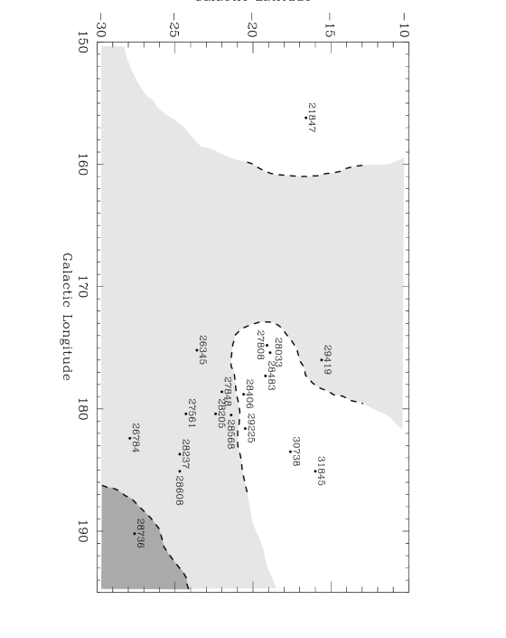
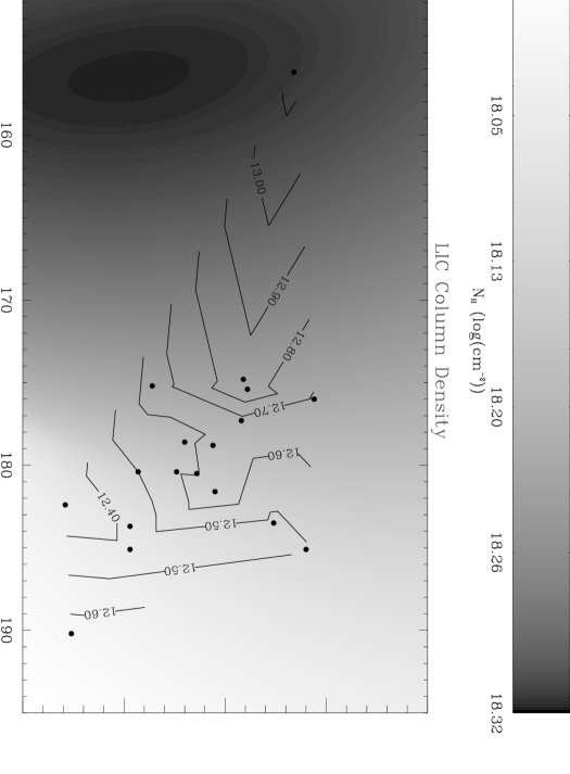
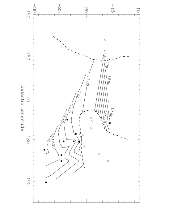
Fig. 8 - Difference in the Mg II column density between pairs of stars as a function of angular separation (degrees). The top panel displays the difference in LIC Mg II column densities (open circles) and 1 $\sigma$ error bars for all pairings of the 18 total targets. The cross-hatch symbols ( $\times$ ) indicate the difference in the predicted LIC H I column densities, provided by the Redfield & Linsky (2000) LIC model. The long dashed line indicates zero change, and the short dashed line indicates a factor of 2 difference in column density. We expect the difference in column density to increase with increasing angular distance. A factor of 2 difference is consistently obtained for objects separated by $\gtrsim~{}8^{\circ}$ . Because we have an indication of the distance to the edge of the LIC (Redfield & Linsky, 2000), we can estimate the physical distance at the edge of the LIC between the lines of sight to a pair of stars from their angular separation. The top axis of the LIC plot shows physical distance in units of parsecs. The bottom panel displays the difference in the Hyades Cloud Mg II column density and 1 $\sigma$ error bars for all pairings of the 10 targets that show Hyades Cloud absorption. The format of the bottom panel is identical to the top. We expect differences in column density to be larger at smaller angular distances, since the Hyades Cloud is at a greater distance than the LIC, meaning the angular distances correspond to larger physical distances.

Fig. 9 - Difference in the Mg II Doppler parameter between pairs of stars as a function of angular separation (degrees). The top panel displays the difference in LIC Mg II Doppler parameters and 1 $\sigma$ error bars for all pairings of the 18 total targets. The long dashed line indicates zero change. Because we have an indication of the distance to the edge of the LIC (Redfield & Linsky, 2000), we can estimate the physical distance at the edge of the LIC between the lines of sight to a pair of stars from their angular separation. The top axis of the LIC plot shows physical distance in units of parsecs. The bottom panel displays the difference in the Hyades Cloud Mg II column density and 1 $\sigma$ error bars for all pairings of the 10 targets that show Hyades Cloud absorption. The format of the bottom panel is identical to the top.